| Issue |
A&A
Volume 688, August 2024
|
|
|---|---|---|
| Article Number | A56 | |
| Number of page(s) | 16 | |
| Section | The Sun and the Heliosphere | |
| DOI | https://doi.org/10.1051/0004-6361/202349020 | |
| Published online | 01 August 2024 | |
One-dimensional, geometrically stratified semi-empirical models of the quiet-Sun photosphere and lower chromosphere⋆
1
Institut für Sonnenphysik, Schöneckstr. 6, 79104 Freiburg, Germany
e-mail: This email address is being protected from spambots. You need JavaScript enabled to view it.
2
Institute for Solar Physics, Department of Astronomy, Stockholm University, AlbaNova University, Centre, 10691 Stockholm, Sweden
Received:
19
December
2023
Accepted:
23
March
2024
Abstract
Context. One-dimensional, semi-empirical models of the solar atmosphere are widely employed in numerous contexts within solar physics, ranging from the determination of element abundances and atomic parameters to studies of the solar irradiance and from Stokes inversions to coronal extrapolations. These models provide the physical parameters (i.e. temperature, gas pressure, etc.) in the solar atmosphere as a function of the continuum optical depth τc. The transformation to the geometrical z scale (i.e. vertical coordinate) is provided via vertical hydrostatic equilibrium.
Aims. Our aim is to provide updated, one-dimensional, semi-empirical models of the solar atmosphere as a function of z, but employing the more general case of three-dimensional magneto-hydrostatic equilibrium (MHS) instead of vertical hydrostatic equilibrium (HE).
Methods. We employed a recently developed Stokes inversion code that, along with non-local thermodynamic equilibrium effects, considers MHS instead of HE. This code is applied to spatially and temporally resolved spectropolarimetric observations of the quiet Sun obtained with the CRISP instrument attached to the Swedish Solar Telescope.
Results. We provide average models for granules, intergranules, dark magnetic elements, and overall quiet-Sun as a function of both τc and z from the photosphere to the lower chromosphere.
Conclusions. We demonstrate that, in these quiet-Sun models, the effect of considering MHS instead of HE is negligible. However, employing MHS increases the consistency of the inversion results before averaging. We surmise that in regions with stronger magnetic fields (i.e. pores, sunspots, network) the benefits of employing the magneto-hydrostatic approximation will be much more palpable.
Key words: magnetohydrodynamics (MHD) / polarization / radiative transfer / Sun: atmosphere / Sun: chromosphere / Sun: granulation
Full Tables A.1–A.4 are available at the CDS via anonymous ftp to cdsarc.cds.unistra.fr (130.79.128.5) or via https://cdsarc.cds.unistra.fr/viz-bin/cat/J/A+A/688/A56
© The Authors 2024
 Open Access article, published by EDP Sciences, under the terms of the Creative Commons Attribution License (https://creativecommons.org/licenses/by/4.0), which permits unrestricted use, distribution, and reproduction in any medium, provided the original work is properly cited.
This article is published in open access under the Subscribe to Open model. This email address is being protected from spambots. You need JavaScript enabled to view it. to support open access publication.
1. Introduction
One-dimensional, semi-empirical models of the solar atmosphere are extremely important and useful for a variety of reasons. They have been used to determine solar abundances (Grevesse et al. 1989; Blackwell et al. 1995; Holweger et al. 1995; Bellot Rubio & Borrero 2002; Borrero 2008) and transition probabilities in spectral lines (Gurtovenko & Kostik 1981; Thevenin 1989, 1990; Borrero et al. 2003) by fitting the solar spectra. They can also be used to study the solar irradiance and its variation during the solar cycle (Unruh et al. 1999; Krivova et al. 2003), or to assist in the extrapolation of magnetic fields from the photosphere toward the chromosphere and corona (Wiegelmann et al. 2013, 2015; Nita et al. 2018, 2023). Finally, they are also very useful as initial guesses to initialise spectropolarimetric inversions (de la Cruz Rodríguez et al. 2016; Borrero et al. 2016; Kuckein et al. 2017; Pastor Yabar et al. 2018; Kuckein 2019; Pastor Yabar et al. 2020; Griñón-Marín et al. 2021), to investigate the formation of spectral lines using contribution and response functions (Bruls & Rutten 1992; Borrero et al. 2017; Milić & van Noort 2017; Vukadinović et al. 2022), to study the turbulent solar magnetic field via the Hanle effect (e.g. Milić & Faurobert 2012), and to determine canonical values of radiative losses in the lower solar atmosphere (Sobotka et al. 2016; Abbasvand et al. 2020).
The most widely used models correspond to average quiet-Sun models, such as HSRA (Gingerich et al. 1971) and HOLMU (Holweger & Mueller 1974). Multi-component models, where the quiet Sun is split into average granular and average intergranular contributions, have also been presented (Borrero & Bellot Rubio 2002). Available models of the magnetized Sun include average network and plage models (Solanki 1986; Solanki & Brigljevic 1992), penumbra (del Toro Iniesta et al. 1994), and umbra (Maltby et al. 1986; Collados et al. 1994). A series of models for various solar features (quiet Sun, sunspots, plage, etc.) have been presented by, among others, Cristaldi & Ermolli (2017), as well as those commonly referred to as VAL-models (Vernazza et al. 1981) and FAL-models (Fontenla et al. 1993, 2009). All the aforementioned models provide the temperature, density, gas pressure, and sometimes the magnetic field and line-of-sight velocity, as a function of the continuum optical depth τc. While some of these models only cover the photosphere (τc ∈ [1, 10−4]), others also include the chromosphere (τc ∈ [10−4, 10−8]) and even part of the transition region (τc < 10−8). One common feature among all these one-dimensional semi-empirical models is that the z scale is calculated using a gas pressure obtained under the assumption of vertical hydrostatic equilibrium (HE). A better estimation of the gas pressure and, therefore, of the z scale can be obtained if we apply three-dimensional magneto-hydrostatic equilibrium (MHS) instead (Borrero et al. 2019, 2021). Although this is particularly the case of regions where the magnetic field is strong (i.e. sunspot, pores, plages, etc.), as a first step, we apply the aforementioned MHS method to the determination of one-dimensional semi-empirical models of the quiet Sun (granules, intergranules and dark magnetic element) here as a function of both the continuum optical depth τc and geometrical height z for the photosphere and lower chromosphere: τc ∈ [15, 2.5 × 10⁻⁶]. To this end, we perform MHS Stokes inversions of spectropolarimetric data at high spatial resolution recorded in the quiet Sun in two spectral lines: one photospheric (treated in local thermodynamic equlibrium) and one photospheric-chromospheric (treated under non-local thermodynamic equilibrium) in order to retrieve the physical properties of solar atmosphere in three dimensions (T(x, y, z), B(x, y, z), Pg(x, y, z), etc.). Granules, intergranules, and dark magnetic elements will then be identified in the data, and average models as a function of z and τc will be calculated.
2. Observations
A region on the quiet-Sun was observed at the disk center (μ = 1.0) on April 24, 2019 with the CRisp Imaging SpectroPolarimeter (Scharmer et al. 2008; de Wijn et al. 2021) attached to the 1-m Swedish Solar Telescope (SST; Scharmer et al. 2003). Although the original data are more exhaustive (i.e. longer time-sequence, larger field of view), here we only describe the portion of the data that was used in our analysis. Other portions of the same dataset have previously been employed in the study of a vortex tube (Fischer et al. 2020) and of a quiet-Sun Ellerman bomb (Kaithakkal et al. 2023).
In our case, we employed the full observed Stokes vector, Iobs = (I, Q, U, V), in the Fe I line at 617.3 nm and the Ca II line at 854.2 nm. The first line was recorded with a wavelength sampling of 35 mÅ across 15 spectral positions, from −245 to +245 mÅ with respect to the line center. The second line was recorded with a varying wavelength sampling, but it was later reinterpolated to a constant sampling of 100 mÅ in 17 spectral positions from −800 to +800 mÅ with respect to the line center. In addition to this, for the Ca II line, an additional wavelength point at +2.4 Å from the line center is used to normalise the spectra. This spectral line features such extended wings that this wavelength is not far enough away to guarantee that the true continuum is reached. In fact, at this wavelength, the Fourier Transform Spectrometer (FTS; Brault & Neckel 1987) atlas intensity reaches only 0.76, which is the number employed for normalization purposes. Table 1 presents the atomic parameters pertaining to these two spectral lines.
Atomic parameters for spectral lines employed in our work.
The field of view in our dataset includes 100 pixels along each spatial dimension on the solar surface with a spatial sampling of 0.059 arcsec (≈44 km). The total field-of-view of 5.9 × 5.9 arcsec2 is sufficient to cover several granular cells’ and intergranules’ lanes. The data calibration was carried out using the SSTRED pipeline (de la Cruz Rodríguez et al. 2015; Löfdahl et al. 2021) and was further processed with the multi-object, multi-frame blind deconvolution code (MOMFBD, Löfdahl 2002; van Noort et al. 2005). In our work, we used a time series of 28 snapshots with a sampling of roughly 30 s, which thus spanned about 15 min of solar evolution.
The spatial resolution of the data is about 0.12 arcsec, and the noise level in the polarization signals is roughly 2 × 10⁻³ in units of the continuum intensity. For context we provide, in Fig. 1, images of the continuum intensity in the Fe I line (top left) and core intensity in the Ca II line (top right) for one of the 28 snapshots in our dataset. In addition, the line-of-sight velocities (or vz) obtained from the line core of both spectral lines are also provided in this figure: Fe I (bottom left), Ca II (bottom right). The line-of-sight velocities were obtained by performing a second-degree polynomial fit in three points centered around the wavelength point with the lowest intensity.
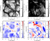 |
Fig. 1. Example of the observations used in this work. Top right: continuum intensity Ic in the Fe I line at 617.3 nm normalized to the average value in the quiet Sun Ic, qs in the same line. Top left: core intensity Icore in the Ca II line at 854.2 nm, normalized to the average value in the quiet Sun Ic, qs. Bottom left: line-of-sight velocity obtained from the core of the Fe I line at 617.3 nm. Bottom right: line-of-sight velocity obtained from the core of the Ca II line at 854.2 nm. Points indicated with the + and ▫ symbols are discussed in Sect. 4.4. |
3. Stokes inversion
The observed Stokes vector Iobs = (I, Q, U, V) as a function of wavelength in the two aforementioned spectral lines is inverted at each spatial position (x, y) on the solar surface with the FIRTEZ Stokes inversion code (Pastor Yabar et al. 2019). This code is currently the only Stokes inversion code capable of employing MHS equilibrium to determine the gas pressure and geometrical height z in the solar atmosphere. For this dataset, we performed six inversion cycles. The reason we needed multiple cycles is explained in Sect. 4.1. The configuration of each inversion cycle is summarized in Table 2. During each cycle, the χ2 merit function between the synthetic Isyn and observed Stokes vector Iobs is minimized using, as a starting atmospheric model, the results from the previous cycle. At each spatial position (x, y), the atmospheric model is discretized along 128 points in the vertical z direction with a step size of Δz = 12 km.
Inversion setup.
During the inversion, the Fe I line is always treated under local thermodynamic equilibrium (LTE), while the Ca II line is treated under non-local thermodynamic equilibrium (NLTE) via departure coefficients (Kaithakkal et al. 2023) in the line opacity and source function (Socas-Navarro et al. 1998, 2000). The departure coefficients for the upper, βupp, and lower, βlow, atomic levels are defined as the ratio between the level populations in NLTE and LTE. Although βupp and βlow for the Ca II line are kept unaltered during all iterations of a given cycle (i.e. akin to the so-called fixed departure coefficients approximation; Ruiz Cobo et al. 2022), they are updated at the end of each cycle. This is done at every point of the full (x, y, z) domain using the SNAPI code (Milić & van Noort 2017, 2018) and assuming complete redistribution in frequencies. SNAPI solves the statistical equilibirum equations with a Ca II atomic model that includes five bound states and one continuum level (Shine & Linsky 1974). Collisional rates are determined using NLTE electron densities and employing a hydrogen model with five bound states plus one continuum level (Osborne & Milić 2021). Since FIRTEZ only uses LTE to determine the electron density Saha (1920), we modified it to consider a new departure coefficient, βe, which is defined as the ratio between the electron density in NLTE and in LTE, so that FIRTEZ can also employ NLTE electron densities when calculating the continuum opacity, mean molecular weight, and gas pressure (i.e. equation of state) during the inversion. Unlike βupp and βlow, βe is not updated after each inversion cycle, but instead kept constant to those of the initial guess model. The reasons for this, along with its implications, are discussed in Sect. 4.2.
During cycles one through three, vertical hydrostatic equilibrium is assumed to determine the gas pressure Pg. At this point, only Stokes I is inverted. This is done by giving zero weight in χ2 to the other Stokes parameters: wi = 1, wq = wu = wv = 0. The number of free parameters (i.e. nodes) are eight for the temperature and eight for the vertical velocity. In order to avoid large grid-to-grid variations in the z direction, we used a Tikhonov regularization (Tikhonov et al. 1995) whereby solutions with large z-derivatives of T(z) and vz(z) are penalized in the χ2 merit-function (de la Cruz Rodríguez et al. 2019).
To initialise the first cycle, an atmospheric model estimation needs to be constructed. In our case, we used the temperature T(z) and gas pressure Pg(z) from the VALC model (Vernazza et al. 1981). The initial departure coefficients βupp(z), βlow(z), and βe(z) are also calculated for this model. The same values are used at each (x, y) position. Vertical velocities vz are initialized differently for each (x, y) and determined via the center-of-gravity method applied to the intensity profile (i.e. Stokes I). The value of vz thus obtained is assumed to be constant with z.
In cycles four through six we fit, along Stokes I, the remaining Stokes parameters (Q, U, and V). Here, the weights in the χ2 merit function given to the linearly polarized Stokes parameters are slowly increased from cycle to cycle (see Table 2). In order to fit all four Stokes parameters, we include nodes in Bx, By, and Bz. During cycle four, we allow for one node in each of the components of the magnetic field. This is increased to two nodes for each component during cycles five and six (see Table 2). The values for Bx, By, and Bz are initialized at the start of the fourth inversion cycle, at each spatial location (x, y), via the weak-field approximation (Jefferies & Mickey 1991) and, to begin with, assumed to be constant in z. The horizontal components of the magnetic field Bx and By are regularized employing the Tikhonov regularization, but using a regularization function in χ2 that penalises deviations from the zero value instead of the vertical derivative (as was the case of T(z) and vz(z) during cycles one through three). With this we try to avoid obtaining large values of the horizontal component of the magnetic field produced by the inversion of low signal-to-noise Q and U profiles that are often seen in quiet-Sun spectropolarimetric observations (Borrero & Kobel 2011, 2012). It is important to note that because the magnetic field is being inverted during cycles four through six and because the gas pressure is also being changed, the fits to Stokes I obtained during the first three cycles can change. In order to make sure that good fits to Stokes I are still obtained during these cycles, we also need to include T and vz during the inversion. This is done, again, with eight nodes in each of these two physical parameters.
Owing to the existence of a non-zero magnetic field in cycles four through six, it is now possible to obtain the gas pressure Pg while accounting for the Lorentz-force term (magneto-hydrostatic equilibrium; Borrero et al. 2019) instead of assuming vertical hydrostatic equilibrium as in cycles one through three. To this end, we employed the procedure described in detail in Borrero et al. (2021; see their Fig. 2) and employed the following boundary conditions: Pg(z = 0) = 2.755 × 10⁵ dyn cm−2 and Pg(z = zmax) = 1.675 dyn cm−2. These boundary conditions apply for every (x, y) pixel. The gas pressure Pg thus obtained is more realistic than the hydrostatic values, and it allows for a reliable inference of the physical parameters (temperature, vertical velocity, and so on) as a function of the Cartesian coordinate z (i.e. geometrical height) instead of using the optical depth τc.
4. Inversion results
4.1. Convergence of non-LTE atomic departure coefficients
In the previous section, we mention that out of the six inversion cycles performed on the data, the first three were carried out with gas pressure Pg resulting from vertical hydrostatic equilibrium, whereas in cycles four through six, the gas pressure Pg was obtained via three-dimensional magneto-hydrostatic equilibrium (see also Table 2). The reason as to why three cycles are needed under each approximation is because at the end of each inversion cycle the departure coefficients are updated, which, in turn, changes the best-fit Stokes profiles and thus also the inferred physical parameters. It takes three cycles of updating the departure coefficients for this procedure to converge. In order to demonstrate this convergence, in Fig. 2 we present the spatial (x, y) average of the ratio between the upper-level departure coefficient, βupp, and the lower-level departure coefficient βlow as a function of the vertical Cartesian coordinate z (i.e. geometrical height) at each inversion cycle. At cycle 1, the departure coefficients correspond to those of the VALC model, and they are the same at every spatial (x, y) pixel because the inversion was initialized with this model everywhere.
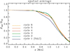 |
Fig. 2. Vertical z stratification of spatial (x, y) average of ratio between the upper level, βupp, and lower level, βlow, departure coefficients. Color-codes indicate the values after each inversion cycle. The initial cycle (dark blue) corresponds to the departure coefficients obtained from the VALC model. |
The reason for illustrating this ratio is because, at visible and near-infrared wavelengths, the source function S(T[z]), where T[z] refers to the temperature dependence along z, is proportional to the ratio βupp(z)/βlow(z). If this ratio remains unchanged in two consecutive inversion cycles it means the inversion can be stopped because no further updates are needed to the departure coefficients and, hence, the temperature T(z). In the case of hydrostatic equilibrium, we reach this convergence after only three cycles, as bespoken by the fact the βupp/βlow is almost identical after cycles two and three.
Once convergence has been achieved, vertical hydrostatic equilibrium is switched off and three-dimensional magneto-hydrostatic equilibrium is used instead. Right at the end of inversion cycle 4, we already have an estimation of the magnetic field B, and, consequently, the gas pressure is calculated under MHS. This of course differs from the gas pressure under HE, thereby yielding very different level populations and thus leading to a new sudden change in the departure coefficients (compare the green curve (cycle three) with the red curve (cycle four) in Fig. 2). Therefore, a new series of inversion cycles under MHS need to be performed until convergence is again achieved. This occurs in cycle six, as departure coefficients after cycle five (orange) and six (yellow) are very similar.
4.2. FIRTEZ equation of state
As already explained in Sect. 3, the atomic level departure coefficients βupp and βlow are determined, using SNAPI, with a NLTE electron density. This is important because βupp and βlow calculated using NLTE electron densities can differ significantly from those calculated using LTE electron densities (see Pastor Yabar et al. in prep.). However, this introduces an inconsistency with FIRTEZ since this code calculates the electron density using Saha’s equation (i.e. LTE; Saha 1920). In order to remove this inconsistency, FIRTEZ has been modified to account for deviations from local thermodynamic equilibrium in the calculation of the electron density via a corresponding departure coefficient, referred to as βe. Unlike the case of the atomic level departure coefficients βupp and βlow, the departure coefficients for the electron density βe are calculated only once for the VALC model and kept the same for all (x, y) pixels in the field of view and for all inversion cycles described in Sect. 3 (see also Table 2). The reason for this is that the inclusion of βe in the determination of the temperature via the Stokes inversion has a minor effect compared to the inclusion of βupp and βlow, and therefore it is much more important to update the latter than the former. This procedure does not fully remove the aforementioned inconsistency, but, judging from the effect that βe has on the temperature inference, we gauge that our systematic error is, at most, of the order of 300 K, which is probably below the systematic uncertainties of chromospheric inversions. In order to illustrate this, in Fig. 3 (left panel) we present the average temperature stratification obtained from the inversion, for all pixels and all times at the end of cycle 1 in three different cases: (a) pure LTE inversion (blue; βe = βupp = βlow = 1); (b) atomic level departure coefficients βupp and βlow, obtained with NLTE electron density, but Stokes inversion using LTE electron density (red; βe = 1; βupp ≠ 1; βlow ≠ 1); and, finally, (c) atomic level departure coefficients βupp and βlow, obtained with NLTE electron density and Stokes inversion also using NLTE electron density (green; βe ≠ 1; βupp ≠ 1; βlow ≠ 1). As can be seen, the largest correction to the temperature (≈1000 − 3000 K) comes from considering NLTE level populations. Including NLTE electron density in the FIRTEZ equation of state typically yields slightly larger temperatures than using LTE electron density, but the differences are contained within 200–300 K. For completeness, Fig. 3 (right panel) provides βe as a function of τc as determined for the VALC model and used in this work.
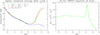 |
Fig. 3. Effects of the equation of state in the retrieval of the temperature. Left panel: spatially and temporally averaged T(log τc) obtained after inversion cycle 1 employing (blue) inversion under LTE; (red) inversion employing NLTE atomic level departure coefficients and LTE equation of state in FIRTEZ; (green) inversion employing NLTE atomic level departure coefficients and NLTE equation of state in FIRTEZ. Right panel: departure coefficient for electron density βe(log τc) used in FIRTEZ equation of state in the third case presented in the left panel. |
4.3. Maps of the physical parameters
In order to illustrate the reliability of the inversion process described in Sect. 3, in this section we present several maps of the physical parameters on the solar surface (x, y) at different optical depths1. The top panels of Fig. 4 show maps of the temperature at log τc = 0 (i.e. low photopshere) and log τc = −5 (i.e. low chromosphere). These two optical depths correspond, approximately, to the height of formation of the continuum in the Fe I line and the core in the Ca II line, respectively, and therefore can be readily compared with the top panels in Fig. 1. The correlation between continuum intensity in Fe I and temperature at log τc = 0 is very clear. Correlations between core intensity in Ca II and temperature at log τc = −5 is lower, albeit still present. This happens because the source function couples more strongly to the local temperature in the photosphere than in the chromosphere, as demonstrated by the fact that the ratio between the upper and lower departure coefficients is very close to unity in the photosphere (see Fig. 2).
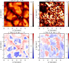 |
Fig. 4. Physical parameters resulting from inversion of Stokes profiles of one of the snapshots described in Sect. 2. Top panels: temperature T(x, y) at log τc = 0 (left) and log τc = −5 (right). Bottom panels: vertical component of velocity vz(x, y) at log τc = −1.5 (left) and log τc = −5 (right). |
The bottom panels in Fig. 4 show the vertical (line-of-sight) velocities vz at optical depths of log τc = −1.5 (i.e. mid photosphere) and log τc = −5 (i.e. low chromosphere). Again, these two optical depths correspond to the height of formation of the core in the Fe I line and the core in the Ca II line, respectively. Consequently, they can be compared with the bottom panels in Fig. 1. A good correlation is also present. Inversion results for the vertical and horizontal components of the magnetic field, Bz and  , at two optical depths (log τc = −1.5, −5) are presented in Fig. 5. As expected from the fact that the polarization signals are much lower in the Ca II line than in the Fe I line, these maps confirm that the magnetic field strength decreases with height. We also note that the horizontal component of the magnetic field at log τc = −1.5 is concentrated mostly inside granular cells.
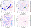 |
Fig. 5. Physical parameters resulting from inversion of Stokes profiles of the same snapshot as in Fig. 4. Top panels: vertical component of magnetic field Bz(x, y) at log τc = −1.5 (left) and log τc = −5 (right). Bottom panels: horizontal component of magnetic field Bh(x, y) at log τc = −1.5 (left) and log τc = −5 (right). |
4.4. Sample fits to the observations
Two examples of the observed (circles), fitted after the cycle 3 (red dashed lines) and fitted after cycle 6 (solid black lines) Stokes profiles, are given in Fig. 6. These correspond to the plus (+) and square (▫) symbols in Figs. 1, 4, and 5, and are located in regions of large positive (Bz > 0) and negative (Bz < 0) polarities. The fits to Stokes I are excellent after cycle 3, but they degrade somewhat after cycle 6, because the polarization profiles are also inverted and are given larger weights than Stokes I in order to infer the three components of the magnetic field. One possibility that was explored, in order to improve to fits to Stokes I, was to fix the temperature T(x, y, z) to those obtained in cycle 3 for the cycles that followed. Unfortunately, this produced even worse fits than the ones presented here in solid black lines because the gas pressure Pg(x, y, z) is being changed despite the temperature being kept the same, resulting in very different T(x, y, log τc). Fortunately, the spatially average temperature stratification as a function of optical depth T(τc) is very similar after cycles 3 and 6, meaning that the errors in the inference of the temperature in the latest cycle that might arise from the misfits to Stokes I cancels out after averaging.
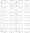 |
Fig. 6. Observed (circles) and fitted Stokes profiles in two examples indicated in Fig. 1. Left panels: results corresponding to pixel indicated by plus (+) symbol. Right panels: results corresponding to pixel indicated by the square (▫). From top to bottom: intensity (Stokes I), linear polarization (Stokes Q and U), and circular polarization (Stokes V). Results after cycle 3 are indicated by the dashed red lines, whereas results after cycle 6 are shown as solid black lines. |
Regarding the polarization signals, we deem the fits to Stokes Q, U, and V after cycle 6 to be good (solid black lines), especially considering that the signals are very weak (below 3% and 1% in circular and linear polarization, respectively) and that we only used two nodes for each of the three components of the magnetic field (see Sect. 3). Of course, cycle 3 produces no polarization signals (dashed red lines) because the magnetic field was not being inverted at this point.
5. Average quet-Sun, granular, intergranular, and dark magnetic element models
The average quiet-Sun model is determined from all 280 000 pixels, within the 5.9″ × 5.9″ field of view, and all 28 snapshots. For the other three models, we identify pixels as belonging to granules, intergranules, or magnetic element depending on two quantities: the vertical component of the velocity and of the magnetic field at an optical depth log τc = −1. We refer to these two quantities as  and
and  , respectively. On the one hand, granular regions are defined as pixels where
  km s−1 and
  G. On the other hand, intergranular regions are defined as pixels where
  km s−1 and
  G. In addition, pixels where
  G are considered to correspond to magnetic elements. An example of the selected pixels using these definitions, for the same snapshot as in the previous figures, is displayed in Fig. 7. We note that the pixels selected as magnetic elements lie mostly in an intergranular region, and therefore it is better to refer to them as dark magnetic element. This is done in order to distinguish them from bright magnetic elements that appear mostly in the network and plage regions. Incidentally, our selection criteria for the dark magnetic element only includes pixels where the magnetic field has positive polarity, and therefore the pixel marked with a square (▫) in previous figures is not actually counted in the average. Once all snapshots are considered, we have a total of about 30 000, 20 000, and 5000 pixels belonging to granules, intergranules, and dark magnetic elements, respectively.
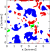 |
Fig. 7. Same as Figs. 1, 4, and 5, but showing regions ascribed to granules (blue), intergranules (red), and to dark magnetic elements (green). |
After granular, intergranular, and dark magnetic element pixels are selected, we construct the average (which corresponds to a spatial and temporal average) in our entire dataset as a function of the vertical coordinate z. This is done for the temperature T(z), gas pressure Pg(z), vertical velocity vz(z), vertical Bz(z), and horizontal 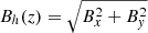 component of the magnetic field. The density is not calculated by averaging, but rather via the equation of state from the averaged temperature and gas pressure. Once the density is known, the opacity and optical depth scales for the spatially and temporarily averaged models can be calculated. The resulting one-dimensional semi-empirical models calculated in this fashion are provided, with a reduced sampling (Δz = 36 km) in Table A.1 (quiet Sun), Table A.2 (granular model), Table A.3 (intergranular model), and Table A.4 (dark magnetic element model). Models tabulated with the original Δz = 12 km sampling can be obtained at the CDS. From all the provided physical parameters, the most useful ones are the thermodynamic and kinematic ones. The temperature and vertical velocities are illustrated in Fig. 8 both as a function of z and log τc. Uncertainties in these models are discussed in Sect. 6. We note that very similar average models would be obtained using only one snapshot from the available time series, but we decided to consider all of them to account for the different stages in the evolution of the studied features.
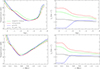 |
Fig. 8. Optical depth stratifciation (log τc; upper panels) and height stratification (z; lower panels) of the temperature (left) and vertical velocity (right) in the four one-dimensional semi-empirical models presented in this work: average quiet-Sun (black), granule (blue), intergranule (red), dark magnetic element (green). |
It is important to note that comparisons with previously existing semi-empirical models should be done with care, especially if those models were obtained from the inversion of spatially and temporally averaged Stokes profiles. As demonstrated by Uitenbroek & Criscuoli (2011) and Milić et al. (2024), for example, due to the non-linearity of the radiative transfer equation, the average atmosphere obtained from the inversion of many Stokes profiles is not necessarily the same as the atmosphere resulting from the inversion of the average of those Stokes profiles. With this in mind, we now focus on some of the properties of the inferred models as presented in this figure.
In the average granular (blue) and interganular (red) models, we observe a temperature reversal between granules and intergranules in the log τc ∈ [ − 1.0, −3.0] or z ∈ [0.25, 0.50] Mm region (see left panels in Fig. 8). This is in agreement with existing models (Borrero & Bellot Rubio 2002; hereafter referred to as BBR2002). This reversal gives rise to what is known as reverse granulation (Gadun et al. 1999; Cheung et al. 2007). The vertical velocities (right panels in Fig. 8) indicate that convective motions are mostly present in the lower photosphere (log τc ≥ −2.0 or z < 0.40 Mm). Above this height, intergranular velocities reverse and turn into upflows, while granules are essentially at rest. This is also in quantitative agreement with BBR2002. The main differences between our granular and integranular models and those from BBR2002 are that (a) we use spatially revolved (with high spatial resolution) observations; (b) we extend the models to the lower chromosphere (log τc ∈ [ − 4, −5.6]); and (c) we also include a more reliable z-scale.
The temperature in the average dark magnetic element (green) features a large temperature enhancement, with respect to the average quiet-Sun model (black), of about 300–400 K at around log τc = −2.0 or z = 0.4 Mm. This is in agreement with network and plage models (Solanki 1986; Solanki & Brigljevic 1992; Lagg et al. 2010). Unlike these aforementioned models, where the temperature enhancement is present at all optical depths, in our model the temperature in the deep photosphere is not enhanced with respect to the average quiet-Sun model. This occurs because our magnetic element lies almost entirely in a dark intergranular lane (see Fig. 7). This also explains why the inferred vertical velocities in the dark magnetic element are so close to that of the intergranules.
The z location of the log τc = 0 (i.e. Wilson depression) can be determined from Tables A.1–A.4. As we can see, the Wilson depression is formed about 30–40 km higher in granules than in intergranules and the dark magnetic element. We note that, as imposed in Sect. 3, the values of the gas pressure at the bottom (z = 0) and top (z = 1524 km) are the same in all three models. We provide a physical parameter in addition to those presented in these tables, which is referred to as Lz (last column in these tables) and corresponds to the vertical component of the Lorentz force. This one is calculated by applying the z component of the momentum equation:
![Mathematical equation: $$ \begin{aligned} L_z = \frac{1}{c} [\boldsymbol{j} \times \boldsymbol{B}]_z = \frac{\partial P_{\rm g}}{\partial z} + \rho g .\end{aligned} $$](/articles/aa/full_html/2024/08/aa49020-23/aa49020-23-eq12.gif) (1)
(1)
Figure 9 (left panel) presents a comparison of the gravity force ρg (solid) and the z-component of the Lorentz force Lz (dashed) in our four average semi-empirical models. Here, we can see that the gravity force dominates by one or two orders of magnitude at most heights. Overall, these results indicate that the spatially and temporally averaged models presented here are in quasi-vertical hydrostatic equilibrium. However, at some particular depths, the z component of the Lorentz force can become comparable to the gravity force. This is the case of the dark magnetic element (green), where at z ≈ 1.0 Mm, the Lorentz force amounts to about 30–40% of the gravity force.
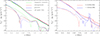 |
Fig. 9. Comparison between gravity force and vertical component of the Lorentz force. Left panel: depth variation of gravity force (solid) and vertical component of the Lorentz force (dashed) in the four one-dimensional semi-empirical models presented in this work: average quiet-Sun (black), granule (blue), intergranule (red), dark magnetic element (green). Lorentz force is given in absolute value so that it can be displayed in a vertical logarithmic scale Right panel: same as above, but considering two individual locations indicated with the + and ▫ symbols in the previous figures. The approximate (x, y) locations of these two pixels in Figs. 4 and 5 are given in parentheses. |
This effect is more noticeable when studying the spatially resolved (i.e. non-averaged) results in (x, y). For instance, in the right panel in Fig. 9 we display again the gravity and Lorentz forces, but now focusing on the two pixels indicated with the + and ▫ symbols in for example Figs. 4, 5. The region where the Lorenz and gravity forces are comparable (Lz ∼ ρg) is now larger. In addition, locally at z ≈ 1.1 Mm (blue) or at z ≈ 1.25 Mm (red), the z component of the Lorentz force can actually be larger than the gravity force. In this regard, these two particular locations selected for Fig. 9 (left panel) are certainly not in vertical hydrostatic equilibrium, with the case of the pixel indicated with + (blue) being particularly striking. We note that in the case of spatially resolved results at every (x, y) location on the map, Pg is not only affected by the vertical component of the Lorentz force, but also by its horizontal (Lx and Ly) components because we consider three dimensional magneto-hydrostatic equilibrium (see Eq. (7) in Borrero et al. 2019).
As shown in Fig. 9 (left panel), the effect of the Lorentz force in the determination of the gas pressure in the one-dimensional (spatially averaged) semi-empirical models and, hence, of the geometrical height scale z of these models, is minimal. Consequently, there is very little difference between having considered vertical hydrostatic or three-dimensional magneto-hydrostatic equilibrium in the determination of the four average models presented here.
Besides the aforementioned discussion about the existence (or non-existence) of quasi-vertical hydrostatic equilibrium in the average and spatially resolved results, there is an additional conceptual difference between the HE and the MHS approaches. As discussed in Borrero et al. (2019; see Sect. 3), imposing hydrostatic equilibrium along the three spatial coordinates (x, y, z) leads to a temperature that does not vary in planes of constant z. Since the temperature is a function of (x, y, z), this immediately implies that hydrostatic equilibrium cannot be maintained along all three Cartesian coordinates. So, in practice it is only imposed vertically (i.e. along z), and the inconsistency along (x, y) is ignored. However, when we account for magneto-hydrostatic equilibrium in three dimensions, we can simultaneously impose vertical and horizontal equilibrium with a temperature that also varies as a function of (x, y), even if the Lorentz force plays a small role. In this regard, the MHS approach is preferable to the HE approach.
6. Uncertainties in the average models
As explained in Sect. 3, the inversion of the observed Stokes profiles Iobs(λ) at each (x, y) pixel on the observed field of view yields the physical parameters (temperature T, line-of-sight velocity vz, etc.) as a function of (x, y, z). Along with it, the FIRTEZ code also yields an error in the estimation of the physical parameters based on the formulation described in Appendix B or Chapter 11.2.1 in Sánchez Almeida (1997) and del Toro Iniesta (2003), respectively. As a measure of the errors in the determination of the physical parameters of the average one-dimensional models presented in this work, we could consider the average of the individual errors at each pixel. Instead of this, it is more representative of the actual uncertainties to consider the standard deviation, around the mean value, from the ensemble of thousands of pixels used to construct these models. These uncertainties are more conservative (i.e. larger) than the former ones because they also include the effects of averaging many pixels that, although they have been ascribed to belong to the same feature (e.g. granule, intergranule, dark magnetic element), they can represent different locations within them (e.g. edge or center of granules) or different stages in the temporal evolution.
Figure 10 presents the average T(z) for each of the models presented: granule (top left; blue lines), intergranule (top right; red lines), dark magnetic elements (bottom left; green lines), and full quiet Sun (bottom right; black lines). These are essentially the same as those in the bottom left panel in Fig. 8, with the exception that we now also include the standard deviations (i.e. uncertainties) in those models as defined above. For comparison purposes, we also display the temperature stratifications as a function of the z coordinate, in a number of widely used models that represent similar features in the solar atmosphere.
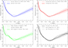 |
Fig. 10. T(z) corresponding to four models presented in this work: average granule (top left; solid blue), average intergranule (top right; solid red), average dark magnetic elements (bottom left; solid green), and average quiet Sun (bottom right; solid black). Standard deviation from the mean values are indicated by the vertical colored lines. The vertical black dashed lines show the location of the τc = 1 level in each of these models. Dashed and dotted color lines represent well-known, one-dimensional semi-empirical models for similar solar structures. The z scale in these models has been shifted so that the τc = 1 coincides with that of the models introduced in this work. |
7. Conclusions and future work
We applied a newly developed FIRTEZ Stokes inversion code in order to invert high spatial resolution spectropolarimetric observations of the quiet Sun in two spectral lines: one photospheric (Fe I 617.3 nm) and one photospheric-chromospheric (Ca II 854.2 nm). While the former spectral line is treated under the assumption of local thermodynamic equilibrium, the latter is treated under non-local thermal equilibrium. The inversion is applied to all pixels on the field of view and for several observing times. Pixels are then selected as belonging to granules (≈30 000 pixels), intergranules (≈30 000 pixels), and dark magnetic element (≈4000 pixels). With this, an average one-dimensional semi-empirical model is constructed for each of these aforementioned structures. In addition, all pixels in the field of view and at all times (≈280 000 pixels) are employed to produce an average model of the entire quiet Sun. Our models are tabulated between z = [0, 1.5] Mm or log τc ≃ [0.75, −5.6]. The vertical scale z is obtained not from the application of vertical hydrostatic equilibrium, but instead from the more general three-dimensional magneto-hydrostatic equilibrium (i.e. including the Lorentz force in the pressure balance). The models presented in this work are therefore particularly useful when the geometrical stratification (i.e. z) is needed instead of the optical depth stratification (τc) or when accurate gas pressures or densities are needed. We find that, while at individual locations the Lorentz force can play an important role (i.e. comparable to or larger than the gravity force), the average models are in a quasi-vertical hydrostatic equilibrium. This will likely not be the case in regions on the solar surface that harbor strong magnetic fields (i.e. network, umbra, penumbra, and so forth). We will provide average models for those structures in the magnetized solar atmosphere in a future paper.
Although our models are originally inferred in the three-dimensional (x, y, z) Cartesian domain, it is better to perform the comparison with actual observables in the τc scale.
Acknowledgments
This research has made use of NASA’s Astrophysics Data System. The Atomic Database (ASD) of the National Institute of Standards and Technology (NIST) was employed in this work. The Institute for Solar Physics is supported by a grant for research infrastructures of national importance from the Swedish Research Council (registration number 2021-00169). The Swedish 1-m Solar Telescope is operated on the island of La Palma by the Institute for Solar Physics of Stockholm University in the Spanish Observatorio del Roque de los Muchachos of the Instituto de Astrofísica de Canarias. APY and JdlCR gratefully acknowledge financial support from the European Union through the European Research Council (ERC) under the Horizon Europe program (MAGHEAT, grant agreement 101088184). Views and opinions expressed are however those of the author(s) only and do not necessarily reflect those of the European Union or the European Research Council. Neither the European Union nor the granting authority can be held responsible for them.
References
- Abbasvand, V., Sobotka, M., Heinzel, P., et al. 2020, ApJ, 890, 22 [Google Scholar]
- Anstee, S. D., & O’Mara, B. J. 1995, MNRAS, 276, 859 [Google Scholar]
- Barklem, P. S., & O’Mara, B. J. 1997, MNRAS, 290, 102 [Google Scholar]
- Barklem, P. S., O’Mara, B. J., & Ross, J. E. 1998, MNRAS, 296, 1057 [Google Scholar]
- Bellot Rubio, L. R., & Borrero, J. M. 2002, A&A, 391, 331 [NASA ADS] [CrossRef] [EDP Sciences] [Google Scholar]
- Blackwell, D. E., Lynas-Gray, A. E., & Smith, G. 1995, A&A, 296, 217 [NASA ADS] [Google Scholar]
- Borrero, J. M. 2008, ApJ, 673, 470 [Google Scholar]
- Borrero, J. M., & Bellot Rubio, L. R. 2002, A&A, 385, 1056 [NASA ADS] [CrossRef] [EDP Sciences] [Google Scholar]
- Borrero, J. M., & Kobel, P. 2011, A&A, 527, A29 [NASA ADS] [CrossRef] [EDP Sciences] [Google Scholar]
- Borrero, J. M., & Kobel, P. 2012, A&A, 547, A89 [NASA ADS] [CrossRef] [EDP Sciences] [Google Scholar]
- Borrero, J. M., Bellot Rubio, L. R., Barklem, P. S., & del Toro Iniesta, J. C. 2003, A&A, 404, 749 [NASA ADS] [CrossRef] [EDP Sciences] [Google Scholar]
- Borrero, J. M., Asensio Ramos, A., Collados, M., et al. 2016, A&A, 596, A2 [NASA ADS] [CrossRef] [EDP Sciences] [Google Scholar]
- Borrero, J. M., Franz, M., Schlichenmaier, R., Collados, M., & Asensio Ramos, A. 2017, A&A, 601, L8 [NASA ADS] [CrossRef] [EDP Sciences] [Google Scholar]
- Borrero, J. M., Pastor Yabar, A., Rempel, M., & Ruiz Cobo, B. 2019, A&A, 632, A111 [NASA ADS] [CrossRef] [EDP Sciences] [Google Scholar]
- Borrero, J. M., Pastor Yabar, A., & Ruiz Cobo, B. 2021, A&A, 647, A190 [NASA ADS] [CrossRef] [EDP Sciences] [Google Scholar]
- Brault, J., & Neckel, H. 1987, Spectral Atlas of Solar Absolute Disk-Averaged and Disk-Center Intensity from 3290 to 12510 Å [Google Scholar]
- Bruls, J. H. M. J., & Rutten, R. J. 1992, A&A, 265, 257 [NASA ADS] [Google Scholar]
- Cheung, M. C. M., Schüssler, M., & Moreno-Insertis, F. 2007, A&A, 461, 1163 [NASA ADS] [CrossRef] [EDP Sciences] [Google Scholar]
- Collados, M., Martinez Pillet, V., Ruiz Cobo, B., del Toro Iniesta, J. C., & Vazquez, M. 1994, A&A, 291, 622 [Google Scholar]
- Cristaldi, A., & Ermolli, I. 2017, ApJ, 841, 115 [NASA ADS] [CrossRef] [Google Scholar]
- de la Cruz Rodríguez, J., Löfdahl, M. G., Sütterlin, P., Hillberg, T., & Rouppe van der Voort, L. 2015, A&A, 573, A40 [NASA ADS] [CrossRef] [EDP Sciences] [Google Scholar]
- de la Cruz Rodríguez, J., Leenaarts, J., & Asensio Ramos, A. 2016, ApJ, 830, L30 [Google Scholar]
- de la Cruz Rodríguez, J., Leenaarts, J., Danilovic, S., & Uitenbroek, H. 2019, A&A, 623, A74 [Google Scholar]
- de Wijn, A. G., de la Cruz Rodríguez, J., Scharmer, G. B., Sliepen, G., & Sütterlin, P. 2021, AJ, 161, 89 [NASA ADS] [CrossRef] [Google Scholar]
- del Toro Iniesta, J. C. 2003, Introduction to Spectropolarimetry (Cambridge, UK: Cambridge University Press) [Google Scholar]
- del Toro Iniesta, J. C., Tarbell, T. D., & Ruiz Cobo, B. 1994, ApJ, 436, 400 [CrossRef] [Google Scholar]
- Edlén, B., & Risberg, P. 1956, Ark. Fys., 100, 553 [Google Scholar]
- Fischer, C. E., Vigeesh, G., Lindner, P., et al. 2020, ApJ, 903, L10 [NASA ADS] [CrossRef] [Google Scholar]
- Fontenla, J. M., Avrett, E. H., & Loeser, R. 1993, ApJ, 406, 319 [Google Scholar]
- Fontenla, J. M., Curdt, W., Haberreiter, M., Harder, J., & Tian, H. 2009, ApJ, 707, 482 [Google Scholar]
- Gadun, A. S., Solanki, S. K., & Johannesson, A. 1999, A&A, 350, 1018 [NASA ADS] [Google Scholar]
- Gingerich, O., Noyes, R. W., Kalkofen, W., & Cuny, Y. 1971, Sol. Phys., 18, 347 [Google Scholar]
- Grevesse, N., Blackwell, D. E., & Petford, A. D. 1989, A&A, 208, 157 [NASA ADS] [Google Scholar]
- Griñón-Marín, A. B., Pastor Yabar, A., Centeno, R., & Socas-Navarro, H. 2021, A&A, 647, A148 [NASA ADS] [CrossRef] [EDP Sciences] [Google Scholar]
- Gurtovenko, E. A., & Kostik, R. I. 1981, A&AS, 46, 239 [NASA ADS] [Google Scholar]
- Holweger, H., & Mueller, E. A. 1974, Sol. Phys., 39, 19 [NASA ADS] [CrossRef] [Google Scholar]
- Holweger, H., Kock, M., & Bard, A. 1995, A&A, 296, 233 [NASA ADS] [Google Scholar]
- Jefferies, J. T., & Mickey, D. L. 1991, ApJ, 372, 694 [NASA ADS] [CrossRef] [Google Scholar]
- Kaithakkal, A. J., Borrero, J. M., Yabar, A. P., & de la Cruz Rodríguez, J. 2023, MNRAS, 521, 3882 [NASA ADS] [CrossRef] [Google Scholar]
- Kramida, A., Ralchenko, Yu., Reader, J., & NIST ASD Team 2023, NIST Atomic Spectra Database (ver. 5.10), [Online] (Gaithersburg, MD: National Institute of Standards and Technology), Available: https://physics.nist.gov/asd [2023, September 1]. [Google Scholar]
- Krivova, N. A., Solanki, S. K., Fligge, M., & Unruh, Y. C. 2003, A&A, 399, L1 [NASA ADS] [CrossRef] [EDP Sciences] [Google Scholar]
- Kuckein, C. 2019, A&A, 630, A139 [NASA ADS] [CrossRef] [EDP Sciences] [Google Scholar]
- Kuckein, C., Diercke, A., González Manrique, S. J., et al. 2017, A&A, 608, A117 [NASA ADS] [CrossRef] [EDP Sciences] [Google Scholar]
- Lagg, A., Solanki, S. K., Riethmüller, T. L., et al. 2010, ApJ, 723, L164 [NASA ADS] [CrossRef] [Google Scholar]
- Löfdahl, M. G. 2002, SPIE Conf. Ser., 4792, 146 [Google Scholar]
- Löfdahl, M. G., Hillberg, T., de la Cruz Rodríguez, J., et al. 2021, A&A, 653, A68 [Google Scholar]
- Maltby, P., Avrett, E. H., Carlsson, M., et al. 1986, ApJ, 306, 284 [Google Scholar]
- Milić, I., & Faurobert, M. 2012, A&A, 539, A10 [NASA ADS] [CrossRef] [EDP Sciences] [Google Scholar]
- Milić, I., & van Noort, M. 2017, A&A, 601, A100 [NASA ADS] [CrossRef] [EDP Sciences] [Google Scholar]
- Milić, I., & van Noort, M. 2018, A&A, 617, A24 [Google Scholar]
- Milić, I., Centeno, R., Sun, X., Rempel, M., & de la Cruz Rodriíguez, J. 2024, A&A, 683, A134 [NASA ADS] [CrossRef] [EDP Sciences] [Google Scholar]
- Nave, G., Johansson, S., Learner, R. C. M., Thorne, A. P., & Brault, J. W. 1994, ApJS, 94, 221 [Google Scholar]
- Nita, G. M., Viall, N. M., Klimchuk, J. A., et al. 2018, ApJ, 853, 66 [NASA ADS] [CrossRef] [Google Scholar]
- Nita, G. M., Fleishman, G. D., Kuznetsov, A. A., et al. 2023, ApJS, 267, 6 [NASA ADS] [CrossRef] [Google Scholar]
- Osborne, C. M. J., & Milić, I. 2021, ApJ, 917, 14 [NASA ADS] [CrossRef] [Google Scholar]
- Pastor Yabar, A., Martínez González, M. J., & Collados, M. 2018, A&A, 616, A46 [NASA ADS] [CrossRef] [EDP Sciences] [Google Scholar]
- Pastor Yabar, A., Borrero, J. M., & Ruiz Cobo, B. 2019, A&A, 629, A24 [NASA ADS] [CrossRef] [EDP Sciences] [Google Scholar]
- Pastor Yabar, A., Martínez González, M. J., & Collados, M. 2020, A&A, 635, A210 [NASA ADS] [CrossRef] [EDP Sciences] [Google Scholar]
- Ruiz Cobo, B., Quintero Noda, C., Gafeira, R., et al. 2022, A&A, 660, A37 [NASA ADS] [CrossRef] [EDP Sciences] [Google Scholar]
- Saha, M. N. 1920, Phil. Mag, 40, 472 [CrossRef] [Google Scholar]
- Sánchez Almeida, J. 1997, ApJ, 491, 993 [CrossRef] [Google Scholar]
- Scharmer, G. B., Bjelksjo, K., Korhonen, T. K., Lindberg, B., & Petterson, B. 2003, SPIE Conf. Ser., 4853, 341 [NASA ADS] [Google Scholar]
- Scharmer, G. B., Narayan, G., Hillberg, T., et al. 2008, ApJ, 689, L69 [Google Scholar]
- Shine, R. A., & Linsky, J. L. 1974, Sol. Phys., 39, 49 [NASA ADS] [CrossRef] [Google Scholar]
- Sobotka, M., Heinzel, P., Švanda, M., et al. 2016, ApJ, 826, 49 [Google Scholar]
- Socas-Navarro, H., Ruiz Cobo, B., & Trujillo Bueno, J. 1998, ApJ, 507, 470 [NASA ADS] [CrossRef] [Google Scholar]
- Socas-Navarro, H., Trujillo Bueno, J., & Ruiz Cobo, B. 2000, ApJ, 530, 977 [NASA ADS] [CrossRef] [Google Scholar]
- Solanki, S. K. 1986, A&A, 168, 311 [NASA ADS] [Google Scholar]
- Solanki, S. K., & Brigljevic, V. 1992, A&A, 262, L29 [NASA ADS] [Google Scholar]
- Thevenin, F. 1989, A&AS, 77, 137 [NASA ADS] [Google Scholar]
- Thevenin, F. 1990, A&AS, 82, 179 [NASA ADS] [Google Scholar]
- Tikhonov, A. N., Goncharsky, A. V., Stepanov, V. V., & Yagola, G. 1995, Numerical Methods for the Solution of Ill-Posed Problems (Springer) [CrossRef] [Google Scholar]
- Uitenbroek, H., & Criscuoli, S. 2011, ApJ, 736, 69 [NASA ADS] [CrossRef] [Google Scholar]
- Unruh, Y. C., Solanki, S. K., & Fligge, M. 1999, A&A, 345, 635 [NASA ADS] [Google Scholar]
- van Noort, M., Rouppe van der Voort, L., & Löfdahl, M. G. 2005, Sol. Phys., 228, 191 [Google Scholar]
- Vernazza, J. E., Avrett, E. H., & Loeser, R. 1981, ApJS, 45, 635 [Google Scholar]
- Vukadinović, D., Milić, I., & Atanacković, O. 2022, A&A, 664, A182 [NASA ADS] [CrossRef] [EDP Sciences] [Google Scholar]
- Wiegelmann, T., Solanki, S. K., Borrero, J. M., et al. 2013, Sol. Phys., 283, 253 [Google Scholar]
- Wiegelmann, T., Neukirch, T., Nickeler, D. H., et al. 2015, ApJ, 815, 10 [NASA ADS] [CrossRef] [Google Scholar]
Appendix A: Atmospheric models
Average quiet-Sun model.
Average granular model.
Average intergranular model.
Average dark magnetic element model.
All Tables
All Figures
|
Fig. 1. Example of the observations used in this work. Top right: continuum intensity Ic in the Fe I line at 617.3 nm normalized to the average value in the quiet Sun Ic, qs in the same line. Top left: core intensity Icore in the Ca II line at 854.2 nm, normalized to the average value in the quiet Sun Ic, qs. Bottom left: line-of-sight velocity obtained from the core of the Fe I line at 617.3 nm. Bottom right: line-of-sight velocity obtained from the core of the Ca II line at 854.2 nm. Points indicated with the + and ▫ symbols are discussed in Sect. 4.4. |
| In the text | |
|
Fig. 2. Vertical z stratification of spatial (x, y) average of ratio between the upper level, βupp, and lower level, βlow, departure coefficients. Color-codes indicate the values after each inversion cycle. The initial cycle (dark blue) corresponds to the departure coefficients obtained from the VALC model. |
| In the text | |
|
Fig. 3. Effects of the equation of state in the retrieval of the temperature. Left panel: spatially and temporally averaged T(log τc) obtained after inversion cycle 1 employing (blue) inversion under LTE; (red) inversion employing NLTE atomic level departure coefficients and LTE equation of state in FIRTEZ; (green) inversion employing NLTE atomic level departure coefficients and NLTE equation of state in FIRTEZ. Right panel: departure coefficient for electron density βe(log τc) used in FIRTEZ equation of state in the third case presented in the left panel. |
| In the text | |
|
Fig. 4. Physical parameters resulting from inversion of Stokes profiles of one of the snapshots described in Sect. 2. Top panels: temperature T(x, y) at log τc = 0 (left) and log τc = −5 (right). Bottom panels: vertical component of velocity vz(x, y) at log τc = −1.5 (left) and log τc = −5 (right). |
| In the text | |
|
Fig. 5. Physical parameters resulting from inversion of Stokes profiles of the same snapshot as in Fig. 4. Top panels: vertical component of magnetic field Bz(x, y) at log τc = −1.5 (left) and log τc = −5 (right). Bottom panels: horizontal component of magnetic field Bh(x, y) at log τc = −1.5 (left) and log τc = −5 (right). |
| In the text | |
|
Fig. 6. Observed (circles) and fitted Stokes profiles in two examples indicated in Fig. 1. Left panels: results corresponding to pixel indicated by plus (+) symbol. Right panels: results corresponding to pixel indicated by the square (▫). From top to bottom: intensity (Stokes I), linear polarization (Stokes Q and U), and circular polarization (Stokes V). Results after cycle 3 are indicated by the dashed red lines, whereas results after cycle 6 are shown as solid black lines. |
| In the text | |
|
Fig. 7. Same as Figs. 1, 4, and 5, but showing regions ascribed to granules (blue), intergranules (red), and to dark magnetic elements (green). |
| In the text | |
|
Fig. 8. Optical depth stratifciation (log τc; upper panels) and height stratification (z; lower panels) of the temperature (left) and vertical velocity (right) in the four one-dimensional semi-empirical models presented in this work: average quiet-Sun (black), granule (blue), intergranule (red), dark magnetic element (green). |
| In the text | |
|
Fig. 9. Comparison between gravity force and vertical component of the Lorentz force. Left panel: depth variation of gravity force (solid) and vertical component of the Lorentz force (dashed) in the four one-dimensional semi-empirical models presented in this work: average quiet-Sun (black), granule (blue), intergranule (red), dark magnetic element (green). Lorentz force is given in absolute value so that it can be displayed in a vertical logarithmic scale Right panel: same as above, but considering two individual locations indicated with the + and ▫ symbols in the previous figures. The approximate (x, y) locations of these two pixels in Figs. 4 and 5 are given in parentheses. |
| In the text | |
|
Fig. 10. T(z) corresponding to four models presented in this work: average granule (top left; solid blue), average intergranule (top right; solid red), average dark magnetic elements (bottom left; solid green), and average quiet Sun (bottom right; solid black). Standard deviation from the mean values are indicated by the vertical colored lines. The vertical black dashed lines show the location of the τc = 1 level in each of these models. Dashed and dotted color lines represent well-known, one-dimensional semi-empirical models for similar solar structures. The z scale in these models has been shifted so that the τc = 1 coincides with that of the models introduced in this work. |
| In the text | |
Current usage metrics show cumulative count of Article Views (full-text article views including HTML views, PDF and ePub downloads, according to the available data) and Abstracts Views on Vision4Press platform.
Data correspond to usage on the plateform after 2015. The current usage metrics is available 48-96 hours after online publication and is updated daily on week days.
Initial download of the metrics may take a while.