| Issue |
A&A
Volume 647, March 2021
|
|
|---|---|---|
| Article Number | L2 | |
| Number of page(s) | 11 | |
| Section | Letters to the Editor | |
| DOI | https://doi.org/10.1051/0004-6361/202140434 | |
| Published online | 10 March 2021 | |
Letter to the Editor
Discovery of CH2CHCCH and detection of HCCN, HC4N, CH3CH2CN, and, tentatively, CH3CH2CCH in TMC-1⋆
1
Grupo de Astrofísica Molecular, Instituto de Física Fundamental (IFF-CSIC), C/ Serrano 121, 28006 Madrid, Spain
e-mail: This email address is being protected from spambots. You need JavaScript enabled to view it.
2
Centro de Desarrollos Tecnológicos, Observatorio de Yebes (IGN), 19141 Yebes, Guadalajara, Spain
3
Observatorio Astronómico Nacional (IGN), C/ Alfonso XII, 3, 28014 Madrid, Spain
Received:
28
January
2021
Accepted:
15
February
2021
Abstract
We present the discovery in TMC-1 of vinyl acetylene, CH2CHCCH, and the detection, for the first time in a cold dark cloud, of HCCN, HC4N, and CH3CH2CN. A tentative detection of CH3CH2CCH is also reported. The column density of vinyl acetylene is (1.2 ± 0.2) × 1013 cm−2, which makes it one of the most abundant closed-shell hydrocarbons detected in TMC-1. Its abundance is only three times lower than that of propylene, CH3CHCH2. The column densities derived for HCCN and HC4N are (4.4 ± 04) × 1011 cm−2 and (3.7 ± 0.4) × 1011 cm−2, respectively. Hence, the HCCN/HC4N abundance ratio is 1.2 ± 0.3. For ethyl cyanide we derive a column density of (1.1 ± 0.3) × 1011 cm−2. These results are compared with a state-of-the-art chemical model of TMC-1, which is able to account for the observed abundances of these molecules through gas-phase chemical routes.
Key words: molecular data / line: identification / ISM: molecules / ISM: individual objects: TMC-1 / astrochemistry
Based on observations carried out with the Yebes 40 m telescope (projects 19A003, 19A010, 20A014, 20D023). The 40 m radio telescope at Yebes Observatory is operated by the Spanish Geographic Institute (IGN, Ministerio de Transportes, Movilidad y Agenda Urbana).
© ESO 2021
1. Introduction
The chemical complexity of the interstellar medium has been demonstrated by the detection of more than 200 different chemical species. In this context, the cold dark core TMC-1 presents an interesting carbon-rich chemistry that led to the formation of long neutral carbon-chain radicals and their anions (see Cernicharo et al. 2020a, and references therein). Cyanopolyynes, which are stable molecules, are also particularly abundant in TMC-1 (see Cernicharo et al. 2020b,c, and references therein). The chemistry of this peculiar object produces a large abundance of the nearly saturated species CH3CHCH2, which could mostly be a typical molecule of hot cores (Marcelino et al. 2007). The polar benzenic ring C6H5CN has also been detected for the first time in space in this object (McGuire et al. 2018), while benzene itself has only so far been been detected toward post-asymptotic giant branch objects (Cernicharo et al. 2001).
Sensitive line surveys are the best tools for unveiling the molecular content of astronomical sources and searching for new molecules. A key element for carrying out a detailed analysis of line surveys is the availability of exhaustive spectroscopic information of the already-known species, their isotopologues, and their vibrationally excited states. The ability to identify the maximum possible number of spectral features leaves the cleanest possible forest of unidentified ones, therefore opening up a chance to discover new molecules and get insights into the chemistry and chemical evolution of the observed objects. In this context we have recently succeeded in discovering, prior to any spectroscopic information from the laboratory, several new molecular species (see, e.g., Cernicharo et al. 2020a,b,c, 2021a,b; Marcelino et al. 2020). Consequently, the astronomical object under study has become a real spectroscopic laboratory. Experience shows that, if the sensitivity of a line survey is sufficiently high, many unknown species will be discovered, providing key information on the ongoing chemical processes in the cloud.
In this Letter we report on the discovery of vinyl acetylene, CH2CHCCH, a species that has been spectroscopically characterized but never detected in space. We also present the detection, for the first time in a cold dark cloud, of HCCN, HC4N, and CH3CH2CN. Ethyl acetylene, CH3CH2CCH, has also been tentatively detected.
2. Observations
New receivers, built within the Nanocosmos project1 and installed at the Yebes 40 m radio telescope, were used for the observations of TMC-1. The Q-band receiver consists of two high electron mobility transistor cold amplifiers covering the 31.0−50.3 GHz range with horizontal and vertical polarizations. Receiver temperatures vary from 17 K at 32 GHz to 25 K at 50 GHz. Eight 2.5 GHz wide fast Fourier transform spectrometers, with a spectral resolution of 38.15 kHz, provide the whole coverage of the Q-band in each polarization. The main beam efficiency varies from 0.6 at 32 GHz to 0.47 at 50 GHz. A detailed description of the system is given in Tercero et al. (2021).
The line survey of TMC-1 (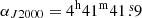 and
and  ) in the Q-band was performed over several sessions. Previous results obtained from the line survey were based on two observing runs, one performed in November 2019 and one in February 2020. They concerned the detection of C3N− and C5N− (Cernicharo et al. 2020b), HC5NH+ (Marcelino et al. 2020), HC4NC (Cernicharo et al. 2020c), and HC3O+ (Cernicharo et al. 2020a). Additional data were taken in October 2020, December 2020, and January 2021 to improve the line survey and to further check the consistency of all observed spectral features. These new data allowed the detection of HC3S+ (Cernicharo et al. 2021a) along with the acetyl cation, CH3CO+ (Cernicharo et al. 2021b), the isomers of C4H3N (Marcelino et al. 2021), and HDCCN (Cabezas et al. 2021).
Two different frequency coverages were used in the line survey, 31.08−49.52 GHz and 31.98−50.42 GHz, to ensure that no spurious spectral ghosts were produced in the down-conversion chain, which down-converts the signal from the receiver to 1−19.5 GHz and then splits it into eight 2.5 GHz bands, which are finally analyzed by the FFTs. The observing procedure was frequency switching with a frequency throw of 10 MHz for the first two runs and 8 MHz for the later ones. The intensity scale (i.e., the antenna temperature,  ) was calibrated using two absorbers at different temperatures and the atmospheric transmission model (ATM; Cernicharo 1985; Pardo et al. 2001). Calibration uncertainties were adopted to be 10%. The nominal spectral resolution of 38.15 kHz was kept for the final spectra. The sensitivity varied across the Q-band from 0.5 to 2.0 mK. All data were analyzed using the GILDAS package2.
3. Results and discussion
The sensitivity of our observations toward TMC-1 (see Sect. 2) is a factor of 10−20 better than previously published line surveys of this source at the same frequencies (Kaifu et al. 2004). This large improvement allowed us to detect a forest of weak lines, most of which arise from the isotopologues of abundant species such as HC3N, HC5N, and HC7N (Cernicharo et al. 2020c). In fact, it was possible to detect many individual lines (Marcelino et al. 2021) from molecular species that had previously only been reported using stacking techniques. Taking into account, on one hand, the large abundances found in TMC-1 for cyanide derivatives of abundant species and, on the other, the presence of nearly saturated hydrocarbons such as CH3CHCH2 (Marcelino et al. 2007), we searched for species such as CH2CHCCH and CH3CH2CCH, as well as for cyanides found previously only in carbon-rich stars (HCCN and HC4N) or in warm molecular clouds (CH3CH2CN). Line identifications in this TMC-1 survey were performed using the MADEX catalogue (Cernicharo 2012), the Cologne Database of Molecular Spectroscopy (CDMS) catalogue (Müller et al. 2005), and the JPL catalogue (Pickett et al. 1998).
3.1. Vinyl acetylene, CH2CHCCH
Spectroscopic constants for CH2CHCCH were derived from a fit to the lines reported by Thorwirth et al. (2004) and implemented in the MADEX code (Cernicharo 2012). We detected six lines with Ka = 0 and 1 (see Fig. 1). Although the observed line intensities (see Table A.1) are low (∼2−3 mK), the column density for this molecule should be particularly large as its dipole moment, μa, is only 0.43 D (Sobolev et al. 1962; Thorwirth & Lichau 2003). Only a Ka = 2 line was marginally detected, corresponding to the 422 − 321 rotational transition. Assuming a uniform source with a radius of 40″ (Fossé et al. 2001) and through a standard rotational diagram, we derived a rotational temperature of 5.0 ± 0.5 K and a column density for vinyl acetylene of (1.2 ± 0.2) × 1013 cm−2. Figure 1 shows the synthetic spectrum of CH2CHCCH computed for the derived rotational temperature and column density (see Appendix A). The comparison with the data shows a very good agreement for all lines, with the exception of the 505 − 404 transition, for which the predicted intensity is nearly a factor of two larger than what is observed. This line is probably affected by a negative spectral feature resulting from the folding of the frequency switching data.
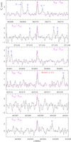 |
Fig. 1. Observed transitions of CH2CHCCH toward TMC-1. The abscissa corresponds to the rest frequency of the lines assuming a vLSR for the source of 5.83 km s−1. Frequencies and intensities for the observed lines are given in Table A.1. The ordinate is the antenna temperature, corrected for atmospheric and telescope losses, in millikelvins (mK). The purple line shows the synthetic spectrum obtained for this species. |
Using the column density of H2 derived by Cernicharo & Guélin (1987), the abundance of CH2CHCCH relative to H2 toward TMC-1 is 1.2 × 10⁻⁹. This abundance is only three times lower than that of propylene (Marcelino et al. 2007), and ten times lower than that of methyl acetylene (Cabezas et al. 2021). Hence, vinyl acetylene is one of the most abundant hydrocarbons in TMC-1 and probably the most abundant compound containing four carbon atoms. It is interesting to compare the abundance of vinyl acetylene with that of vinyl cyanide. We analyzed the lines of CH2CHCN covered by our Q-band data. We derived a rotational temperature of 4.5 ± 0.3 K, and N(CH2CHCN) = (6.5 ± 0.5) × 1012 cm−2 (see Appendix C). Hence, the abundance ratio between the acetylenic and cyanide derivatives of ethylene (CH2CH2) is 1.8 ± 0.4, which suggests that ethylene could be a likely precursor of CH2CHCCH and CH2CHCN through reactions with CCH and CN, respectively (see Sect. 3.4 for more details).
We searched for CH3CH2CCH in our survey. Figure 2 shows the resulting spectrum from stacking the lines of this species covered in our data (see details in Appendix B). The whole set of individual lines is shown in Fig. B.1. We consider this molecule to be tentatively detected with a column density of 9 × 1011 cm−2. We also detected ethyl cyanide, CH3CH2CN, in TMC-1 (see Sect. 3.3) with a column density of 1011 cm−2. Hence, assuming that CH3CH2CCH in TMC-1 is detected, the abundance ratio CH3CH2CCH/CH3CH2CN is ∼9.
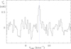 |
Fig. 2. Line profile for CH3CH2CCH toward TMC-1 from stacking the signal from the transitions of this species in the 31−50 GHz frequency range. The abscissa corresponds to the local standard of rest velocity. The ordinate is the antenna temperature, corrected for atmospheric and telescope losses, in mK. The observed spectra from the individual lines are shown in Fig. B.1. |
3.2. HCCN and HC4N
The cyano methylene radical, HCCN, was detected toward the carbon-rich star IRC +10216 by Guélin & Cernicharo (1991). The molecule has been observed in the laboratory by several authors (Saito et al. 1984; Endo & Ohshima 1993; McCarthy et al. 1995; Allen et al. 2001). Its dipole moment is 3.04 D (Inostroza et al. 2012). Given the large abundance of cyanopolyynes in TMC-1 (e.g., Cernicharo et al. 2020c), HCCN could be expected in this source, although it was searched for by McGonagle & Irivine (1996) with no success. Several of its rotational transitions, which show significant hyperfine splitting, are within the frequency range of our TMC-1 survey. All of them were detected, as shown in Fig. 3 (see Table A.1). This is the first time HCCN has been detected in cold interstellar clouds. The range of level energies covered by the observed transitions, 1.6−3.7 K, did not allow us to build a reliable rotational diagram. We adopted the rotational temperature derived for CH2CHCN (4.5 ± 0.5 K; see Sect. 3.1) and computed a synthetic spectrum with the column density as a free parameter. The best fit was obtained for a column density of (4.4 ± 0.4) × 1011 cm−2. As shown in Fig. 3, the match between the model and the observations is very good.
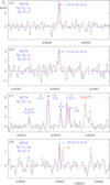 |
Fig. 3. Observed lines of HCCN in our Q-band survey toward TMC-1. The abscissa corresponds to the rest frequency assuming a vLSR of the source of 5.83 km s−1. The ordinate is the antenna temperature, corrected for atmospheric and telescope losses, in mK. The violet line shows the synthetic spectrum computed for Tr = 4.5 K and N(HCCN) = 4.4 × 1011 cm−2. For the sake of clarity, only the upper quantum numbers F1 and F are provided in panel c. |
In addition to HCCN, the linear cyano ethynyl-methylene radical, HC4N, was also detected in IRC +10216 (Cernicharo et al. 2004). Spectroscopic information on this molecule (Tang et al. 1999) was implemented in MADEX. Its dipole moment is 4.33 D (Ikuta et al. 2000). The observed lines toward TMC-1 are shown in Fig. 4. From those lines and the model fitting procedure, it is possible to derive a rotational temperature of 4 ± 1 K and a column density of (3.7 ± 0.4) × 1011 cm−2. Figure 4 shows the synthetic spectrum corresponding to these parameters. The agreement with the observations is very good. This is the first time that this species has been detected in a cold dark cloud.
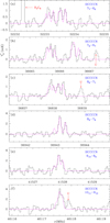 |
Fig. 4. Selected lines of HC4N in the 31−50 GHz frequency range toward TMC-1. The abscissa corresponds to the rest frequency assuming a vLSR for TMC-1 of 5.83 km s−1. The ordinate is the antenna temperature, corrected for atmospheric and telescope losses, in mK. The violet line shows the synthetic spectrum computed for Tr = 4.0 K and N(HC4N) = 3.7 × 1011 cm−2. |
We searched for the bent and cyclic isomers of HC4N (McCarthy et al. 1999a,b) without success. We derived 3σ upper limits to their column densities of 1.5 × 1011 cm−2 and 1.0 × 1011 cm−2, respectively. It is interesting to note that these two isomers have a very different molecular structure relative to linear HC4N (Cernicharo et al. 2004). Hence, they are probably not formed in the reaction between CH and HC3N, which is the main pathway to the linear isomer. Finally, we searched for the related radicals CCN (Kakimoto & Kasuya 1982; Ohshima & Endo 1995) and C4N (McCarthy et al. 2003). However, due to their low permanent dipole moment (Pd. & Chandra 2001; Fiser & Polák 2013), we obtained very conservative 3σ upper limits to their abundances of 1.8 × 1012 cm−2 and 4.0 × 1013 cm−2, respectively.
The abundance ratio HCCN/HC4N derived in TMC-1 is 1.2 ± 0.3, which is very different than that derived in the carbon-star envelope IRC +10216 (∼9; Cernicharo et al. 2004). In IRC +10216, this abundance ratio is a factor of two larger than the HC2n + 1N/HC2n + 3N decrement observed for cyanopolyynes (Cernicharo et al. 2004), while in TMC-1 the HCCN/HC4N ratio is two to three times lower than that of the cyanopolyyne decrement. The different behavior in TMC-1 compared to IRC +10216 is probably caused by differences in the abundances of the precursors of HCCN and HC4N (see Sect. 3.4).
3.3. CH3CH2CN
This molecule is typical of warm molecular clouds, where it produces a forest of lines arising from all its isotopologues and low-energy vibrational excited states (Demyk et al. 2007; Daly et al. 2013). It was searched for in TMC-1 by Minh & Irvine (1991) without success. More recently, Lee et al. (2021) used stacking techniques, providing an upper limit to its column density in TMC-1 of 4 × 1011 cm−2. We searched for the lines of this molecule in our TMC-1 Q-band survey. Figure B.2 shows the six lines with Ka = 0 and 1 detected. All of them appear at 4−5σ levels. The Ka = 2 lines are too weak to be detected with the sensitivity of our survey.
We computed a synthetic spectrum using the rotational temperature derived for CH2CHCN (4.5 K; see Appendix C) and a column density of N(CH3CH2CN) = 1.1 × 1011 cm−2 (with an estimated error of 30%). The match between the observations and the model is very reasonable. We derived abundance ratios CH2CHCN/CH3CH2CN = 65 ± 20 and CH2CHCCH/CH3CH2CCH = 120 ± 40. It is interesting to compare the abundance ratio between vinyl cyanide and ethyl cyanide in TMC-1 and that in Orion KL. In the latter source it is 0.06 (López et al. 2014), which is a factor of ∼1100 smaller than in TMC-1. The spatial distribution of both molecules in Orion KL has been analyzed by Cernicharo et al. (2016). Both species arise in regions with temperatures of 100 and 350 K. The huge difference in this abundance ratio tells us about the different chemical processes prevailing in cold and warm molecular clouds. While the chemistry is dominated by the contribution of the evaporating ices covering dust grains in objects such as Orion KL, reactions between radicals and neutrals in cold dark clouds play a key role in producing these molecules.
3.4. Chemistry of detected molecules
After the discovery of abundant propylene in TMC-1 (Marcelino et al. 2007), the detection of an even larger, partially saturated, and abundant hydrocarbon, such as vinyl acetylene, in the same cloud brings to light the existence of a rich organic chemistry in cold dark clouds, going beyond the long-known presence of unsaturated carbon chains. Moreover, just as the hydrocarbons CH3CCH and CH2CCH2 act as precursors of the various nitriles C4H3N found in TMC-1 (Marcelino et al. 2021), CH2CHCCH emerges as a very likely candidate precursor of the large nitriles with molecular formula C5H3N that have recently been claimed in TMC-1 (Lee et al. 2021).
To get insight into the formation mechanism of CH2CHCCH and the other molecules covered in this study, we ran a pseudo-time-dependent gas-phase chemical model that adopts typical parameters of cold dark clouds (see, e.g., Agúndez & Wakelam 2013). We used the chemical network RATE12 from the UMIST database (McElroy et al. 2013), augmented with reactions relevant for the molecules of interest in this work, which are discussed below.
Vinyl acetylene is formed in the model through the neutral-neutral gas-phase reactions C2 + C2H6, CH + C3H4 (where C3H4 stands for the two isomers CH3CCH and CH2CCH2), and C2H + C2H4. These reactions have been found to be rapid at low temperatures (Canosa et al. 2007; Daugey et al. 2005; Bowman et al. 2012), and branching ratios have been measured for some of them (Loison & Bergeat 2009; Goulay et al. 2009; Bowman et al. 2012). Vinyl acetylene is predicted to form with a peak abundance of ∼10−9 relative to H2 (see Fig. 5), in good agreement with the value derived from observations. We also investigated whether cyanide derivatives of CH2CHCCH can be formed through the reaction CN + CH2CHCCH, which has been found to be rapid for temperatures down to 174 K (Yang et al. 1992). The peak abundance calculated for the generic species C5H3N, which accounts for different possible isomers, is a few times 10−10 relative to H2, somewhat above the observed abundance, which means that the reaction between CN and vinyl acetylene is a viable route to the C5H3N isomers found in TMC-1 (Lee et al. 2021). Information on the kinetics of this reaction down to very low temperatures would be highly valuable to validate this mechanism.
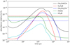 |
Fig. 5. Calculated fractional abundances of assorted molecules relevant to this study as a function of time. Horizontal dashed lines correspond to observed values. |
Ethyl cyanide can also be formed efficiently in the gas phase in cold dark cloud conditions. In our chemical model the main route involves the radiative association between  and CH3CN and the dissociative recombination of the ion C2H5CNH+ with electrons, both of which have measured rate constants (Anicich 1993; Vigren et al. 2010). The calculated peak abundance is ∼10−10 relative to H2 (see Fig. 5), which is around ten times higher than the observed value. The chemical network probably misses some important reactions of destruction of CH3CH2CN (e.g., with neutral atoms or ions) which could explain the abundance overestimation.
We finally discuss the formation of the allenic molecules HCCN and HC4N in TMC-1. The chemical network that involves HCCN is mostly taken from Loison et al. (2015), while that for HC4N is assumed to be similar. The chemical model predicts HCCN to be around ten times more abundant than HC4N (see Fig. 5), in contrast with observations that find both molecules to have similar abundances. The reason for this is that the main routes to HCCN and HC4N are the reactions CH + HCN/HNC and CH + HC3N, respectively (with rate constants based on Zabarnick et al. 1991), and the chemical model predicts that HCN and HNC together are around ten times more abundant than HC3N. However, observations indicate that HC3N is as abundant as HCN and HNC in TMC-1 (e.g., Agúndez & Wakelam 2013), and therefore if the reactions CH + HCN/HNC and CH + HC3N are the main pathways to HCCN and HC4N, respectively, one would expect similar abundances for HCCN and HC4N, in agreement with observations. The higher HCCN/HC4N observed in IRC +10216 is probably explained by the higher abundance of HCN compared to HC3N in this source.
Acknowledgments
We thank Ministerio de Ciencia e Innovación of Spain (MICIU) for funding support through projects AYA2016-75066-C2-1-P, PID2019-106110GB-I00, PID2019-107115GB-C21/AEI/10.13039/501100011033, and PID2019-106235GB-I00. We also thank ERC for funding through grant ERC-2013-Syg-610256-NANOCOSMOS. M.A. thanks MICIU for grant RyC-2014-16277.
References
- Agúndez, M., & Wakelam, V. 2013, Chem. Rev., 113, 8710 [Google Scholar]
- Allen, M. D., Evenson, K. M., & Brown, J. M. 2001, J. Mol. Spectr., 209, 143 [CrossRef] [Google Scholar]
- Anicich, V. G. 1993, J. Phys. Chem. Ref. Data, 22, 1469 [NASA ADS] [CrossRef] [Google Scholar]
- Bestmann, G., & Dreizler, H. 1985, Z. Naturforsch., 40a, 263 [CrossRef] [Google Scholar]
- Bowman, J., Goulay, F., Leone, S. R., & Wilson, K. R. 2012, J. Phys. Chem. A, 116, 3907 [CrossRef] [Google Scholar]
- Cabezas, C., Endo, Y., Roueff, E., et al. 2021, A&A, 646, L1 [NASA ADS] [CrossRef] [EDP Sciences] [Google Scholar]
- Canosa, A., Páramo, A., Le Picard, S. D., & Sims, I. R. 2007, Icarus, 187, 558 [NASA ADS] [CrossRef] [Google Scholar]
- Cernicharo, J. 1985, Internal IRAM Report (Granada: IRAM) [Google Scholar]
- Cernicharo, J. 2012, EAS Publ. Ser., 58, 251 [Google Scholar]
- Cernicharo, J., & Guélin, M. 1987, A&A, 176, 299 [Google Scholar]
- Cernicharo, J., Heras, A. M., Tielens, A. G. G. M., et al. 2001, ApJ, 546, L123 [NASA ADS] [CrossRef] [Google Scholar]
- Cernicharo, J., Guélin, M., & Pardo, J. R. 2004, ApJ, 615, L145 [NASA ADS] [CrossRef] [Google Scholar]
- Cernicharo, J., Kisiel, Z., Tercero, B., et al. 2016, A&A, 587, L4 [NASA ADS] [CrossRef] [EDP Sciences] [Google Scholar]
- Cernicharo, J., Marcelino, N., Agúndez, M., et al. 2020a, A&A, 642, L17 [NASA ADS] [CrossRef] [EDP Sciences] [Google Scholar]
- Cernicharo, J., Marcelino, N., Pardo, J. R., et al. 2020b, A&A, 641, L9 [NASA ADS] [CrossRef] [EDP Sciences] [Google Scholar]
- Cernicharo, J., Marcelino, N., Agúndez, M., et al. 2020c, A&A, 642, L8 [NASA ADS] [CrossRef] [EDP Sciences] [Google Scholar]
- Cernicharo, J., Cabezas, C., Endo, Y., et al. 2021a, A&A, 646, L3 [EDP Sciences] [Google Scholar]
- Cernicharo, J., Cabezas, C., Bailleux, S., et al. 2021b, A&A, 646, L7 [NASA ADS] [CrossRef] [EDP Sciences] [Google Scholar]
- Daly, A. M., Bermúdez, C., López, A., et al. 2013, ApJ, 768, 81 [NASA ADS] [CrossRef] [Google Scholar]
- Daugey, N., Caubet, P., Retail, B., et al. 2005, Phys. Chem. Chem. Phys., 7, 2921 [CrossRef] [Google Scholar]
- Demaison, J., Boucher, D., Burie, J., & Dubrulle, A. 1983, Z. Naturforsch., 38, 447 [CrossRef] [Google Scholar]
- Demyk, K., Mäder, H., Tercero, B., et al. 2007, A&A, 466, 255 [NASA ADS] [CrossRef] [EDP Sciences] [Google Scholar]
- Endo, Y., & Ohshima, Y. 1993, J. Chem. Phys., 98, 6618 [CrossRef] [Google Scholar]
- Fiser, J., & Polák, R. 2013, Chem. Phys., 425, 126 [CrossRef] [Google Scholar]
- Fossé, D., Cernicharo, J., Gerin, M., & Cox, P. 2001, ApJ, 552, 168 [Google Scholar]
- Goulay, F., Trevitt, A. J., Meloni, G., et al. 2009, J. Am. Chem. Soc., 131, 993 [CrossRef] [Google Scholar]
- Guélin, M., & Cernicharo, J. 1991, A&A, 244, L21 [NASA ADS] [Google Scholar]
- Ikuta, S., Tsuboi, T., & Aoki, K. 2000, J. Mol. Struct., 528, 297 [CrossRef] [Google Scholar]
- Inostroza, N., Huang, X., & Lee, T. J. 2012, J. Chem. Phys., 135, 244310 [NASA ADS] [CrossRef] [Google Scholar]
- Kaifu, N., Ohishi, M., Kawaguchi, K., et al. 2004, PASJ, 56, 69 [Google Scholar]
- Kakimoto, M., & Kasuya, T. 1982, J. Mol. Spectr., 94, 380 [NASA ADS] [CrossRef] [Google Scholar]
- Landsberg, B. M., & Suenram, R. D. 1983, J. Mol. Spectr., 98, 210 [NASA ADS] [CrossRef] [Google Scholar]
- Lee, K. L. K., Loomis, R. A., Burkhardt, A. M., et al. 2021, ApJ, 908, L11 [CrossRef] [Google Scholar]
- Loison, J.-C., & Bergeat, A. 2009, Phys. Chem. Chem. Phys., 11, 655 [CrossRef] [Google Scholar]
- Loison, J.-C., Hébrard, E., Dobrijevic, M., et al. 2015, Icarus, 247, 218 [NASA ADS] [CrossRef] [Google Scholar]
- López, A., Tercero, B., Kisiel, Z., et al. 2014, A&A, 572, A44 [NASA ADS] [CrossRef] [EDP Sciences] [Google Scholar]
- Marcelino, N., Cernicharo, J., Agúndez, M., et al. 2007, ApJ, 665, L127 [Google Scholar]
- Marcelino, N., Agúndez, M., Tercero, B., et al. 2020, A&A, 643, L6 [NASA ADS] [CrossRef] [EDP Sciences] [Google Scholar]
- Marcelino, N., Tercero, B., Agúndez, M., & Cernicharo, J. 2021, A&A, 646, L9 [NASA ADS] [CrossRef] [EDP Sciences] [Google Scholar]
- McCarthy, M. C., Gottlieb, C. A., Cooksy, A. L., & Thaddeus, P. 1995, J. Chem. Phys., 103, 7779 [CrossRef] [Google Scholar]
- McCarthy, M. C., Apponi, A. J., Gordon, V. D., et al. 1999a, J. Chem. Phys., 111, 6750 [CrossRef] [Google Scholar]
- McCarthy, M. C., Grabow, J.-U., Travers, M. J., et al. 1999b, ApJ, 513, 305 [CrossRef] [Google Scholar]
- McCarthy, M. C., Fuchs, G. W., Kucera, J., et al. 2003, J. Chem. Phys., 118, 3549 [CrossRef] [Google Scholar]
- McElroy, D., Walsh, C., Markwick, A. J., et al. 2013, A&A, 550, A36 [NASA ADS] [CrossRef] [EDP Sciences] [Google Scholar]
- McGonagle, D., & Irivine, W. M. 1996, A&A, 310, 970 [Google Scholar]
- McGuire, B. A., Burkhardt, M., Kalenskii, S., et al. 2018, Science, 359, 202 [NASA ADS] [CrossRef] [Google Scholar]
- Minh, Y. C., & Irvine, W. M. 1991, Astrophys. Space Sci., 175, 165 [NASA ADS] [CrossRef] [Google Scholar]
- Müller, H. S. P., Schlöder, F., Stutzki J., et al. 2005, J. Mol. Struct., 742, 215 [NASA ADS] [CrossRef] [Google Scholar]
- Ohshima, Y., & Endo, Y. 1995, J. Mol. Spectr., 172, 225 [NASA ADS] [CrossRef] [Google Scholar]
- Pardo, J. R., Cernicharo, J., & Serabyn, E. 2001, IEEE Trans. Antennas Propag., 49, 12 [Google Scholar]
- Pickett, H. M., Poynter, R. L., Cohen, E. A., et al. 1998, J. Quant. Spectr. Rad. Transf., 60, 883 [Google Scholar]
- Pd., R., & Chandra, P. 2001, J. Chem. Phys., 114, 1589 [NASA ADS] [CrossRef] [Google Scholar]
- Saito, S., Endo, Y., & Hirota, E. 1984, J. Chem. Phys., 80, 1427 [NASA ADS] [CrossRef] [Google Scholar]
- Sobolev, G. A., Shcherbakov, A. M., & Akishin, P. A. 1962, Opt. Spectr., 12, 78 [Google Scholar]
- Steber, A. L., Harris, B. J., Neill, J. L., et al. 2012, J. Mol. Spectr., 280, 3 [CrossRef] [Google Scholar]
- Tang, J., Sumiyoshi, Y., & Endo, Y. 1999, Chem. Phys. Lett., 315, 69 [CrossRef] [Google Scholar]
- Tercero, F., López-Pérez, J. A., Gallego, J. D., et al. 2021, A&A, 645, A37 [EDP Sciences] [Google Scholar]
- Thorwirth, S., & Lichau, H. 2003, A&A, 398, L11 [NASA ADS] [CrossRef] [EDP Sciences] [Google Scholar]
- Thorwirth, S., Müller, H. S. P., Lichau, H., et al. 2004, J. Mol. Struct., 695, 263 [CrossRef] [Google Scholar]
- Vigren, E., Hamberg, M., Zhaunerchyk, V., et al. 2010, ApJ, 722, 847 [NASA ADS] [CrossRef] [Google Scholar]
- Yang, D. L., Yu, T., Wang, N. S., & Lin, M. C. 1992, Chem. Phys., 160, 317 [CrossRef] [Google Scholar]
- Zabarnick, S., Fleming, J. W., & Lin, M. C. 1991, Chem. Phys., 150, 109 [NASA ADS] [CrossRef] [Google Scholar]
Appendix A: Line parameters for CH2CHCCH and model fitting procedure
Line parameters were derived for CH2CHCCH by fitting a Gaussian line profile to the observed lines. A velocity range of ±20 km s−1 around each feature was considered for the fit after a polynomial baseline was removed. The derived line parameters are given in Table A.1.
Observed line parameters for CH2CHCCH, HCCN, HC4N, and CH3CH2CN.
For the other species we show the synthetic spectrum resulting from the best fit model to all the lines computed using the MADEX code (Cernicharo 2012). We assumed a homogeneous rotational temperature for all rotational levels, a source of uniform brightness with a radius of 40″ (Fossé et al. 2001), and a full linewidth at half power intensity of 0.6 km s−1, which represents a good averaged value to the linewidth of all observed lines. A fit to the observed line profiles and intensities provide the rotational temperature and the column density for the observed species. The final parameters derived in this way should be very similar to those derived from a standard rotational diagram. However, this model fit allows us to compare the modeled line profiles with those of the observations, which is particularly interesting when the rotational transitions exhibit hyperfine structure, as is the case for HCCN, HC4N, and, to a lesser extent, CH3CH2CN.
Appendix B: Ethyl acetylene and ethyl cyanide
We searched for the lines of ethyl acetylene, CH3CH2CCH, a molecule for which accurate laboratory data are available up to 317.7 GHz (Demaison et al. 1983; Landsberg & Suenram 1983; Bestmann & Dreizler 1985; Steber et al. 2012) and which has moderate dipole moments of μa = 0.763 D and μb = 0.17 D (Landsberg & Suenram 1983). The barrier to internal rotation is very high (Bestmann & Dreizler 1985), and therefore the ground state does not show significant splitting between the A and E species. Of the ten lines expected for this molecule in the Q-band, five are detected at a 3σ level, two are blended with other weak features slightly shifted in frequency, and three are too weak. Using stacking techniques (see below) and removing the blended lines, which could introduce a significant bias in the final spectrum, we detected a signal at 5σ at the correct velocity, as shown in Fig. 2. However, we have no explanation for the lack of emission at the frequency of the 505 − 404 transition other than that the data are too noisy at its frequency (see Fig. B.1). It is expected to be the strongest feature for the parameters we used for the synthetic spectrum (Tr = 5 K, N(CH3CH2CCH) = 9 × 1011 cm−2).
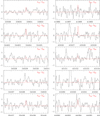 |
Fig. B.1. Observed lines of CH3CH2CCH in the Q-band toward TMC-1. The abscissa corresponds to the rest frequency assuming a local standard of rest velocity of 5.83 km s−1. The ordinate is the antenna temperature, corrected for atmospheric and telescope losses, in mK. The red line shows the synthetic spectrum obtained using the parameters derived from a rotational diagram of the observed lines (Tr = 5 K and N(CH3CH2CCH) = 9.0 × 1011 cm−2). The rotational quantum numbers are provided in the upper right corners of each panel. |
For CH3CH2CCH, all the expected strongest lines in the Q-band are shown in Fig. B.1, and Fig. 2 shows the resulting stacked profile. The stacking procedure we used is rather simple: a velocity range of ±20 km s−1 was selected for each line and the noise, σ, outside 5.83 ± 0.5 km s−1 was computed (with known and unknown lines in each individual spectrum blanked). The data were normalized to the expected intensity of each transition computed under local thermodynamic equilibrium for a rotational temperature of 5 K, the same as the value derived for CH2CHCCH. Finally, all the data were multiplied by the expected intensity of the strongest transition in the sample. The lines are optically thin, and hence the intensity of all lines scale in the same way with the assumed column density. Each individual spectrum was weighted as 1/ , where σN now contains the normalization intensity factor. All rotational transitions falling in the frequency ranges where our data have the highest sensitivity were detected (transitions 414 − 313, 404 − 303, 413 − 312, 515 − 414, and 524 − 523). Two of the observed transitions are heavily blended (422 − 321 and 514 − 413) and were excluded from the stacked spectrum. Two Ka = 2 transitions, which are expected to be weak, were not detected (423 − 322 and 523 − 422) but were included in the data stacking with the corresponding weights, as explained above. The data for the strongest rotational transition, the 505 − 404, have a sensitivity of 0.6 mK. The expected intensity is 1.3 mK. This rotational transition was included in the stacked spectrum, although it is clearly not detected at the noise level of the data. Figure 2 shows the resulting spectrum from this procedure. A feature, at exactly the velocity of the cloud, appears at a 5σ level (σ = 0.16 mK). Although a positive detection of ethyl acetylene is highly possible, we consider it as tentative. Longer integration times are needed to confirm the detection of this species.
In our survey we observed a large number of unidentified lines at the level of 1−5 mK (see Figs. 1, 3, 4, and B.1). Moreover, the isotopologues of abundant species contribute with several hundred lines. Consequently, stacking techniques that could compete in sensitivity with our survey may provide false positive or negative results for low abundant molecular species. An example is the case of CH3CH2CN, which was detected in our work (see Sect. 3.3 and Fig. B.2), while only upper limits were obtained by Lee et al. (2021). The observed lines of CH3CH2CN, together with the best model fit to the observed emission, are shown in Fig. B.2.
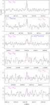 |
Fig. B.2. Observed lines of CH3CH2CN in the 31−50 GHz frequency range toward TMC-1. The abscissa corresponds to the rest frequency assuming a local standard of rest velocity of 5.83 km s−1. The ordinate is the antenna temperature, corrected for atmospheric and telescope losses, in mK. The violet line shows the synthetic spectrum computed for Tr = 4.5 K and N(CH3CH2CN) = 1.1 × 1011 cm−2. |
Appendix C: Vinyl cyanide, CH2CHCN
Vinyl cyanide produces a very rich spectrum in the 31−50 GHz range, with most of its lines exhibiting the hyperfine structure due to the nitrogen nucleus. All the observed lines are shown in Fig. C.1. The model fitting procedure provides a rotational temperature of 4.5 ± 0.5 K and a column density of (6.5 ± 0.5) × 1012 cm−2. Its abundance relative to vinyl acetylene and ethyl cyanide is discussed in Sects. 3.1, 3.3, and 3.4.
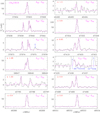 |
Fig. C.1. Observed lines of CH2CHCN in the 31−50 GHz frequency range toward TMC-1. The abscissa corresponds to the rest frequency assuming a local standard of rest velocity of 5.83 km s−1. The ordinate is the antenna temperature, corrected for atmospheric and telescope losses, in mK. The violet line shows the synthetic spectrum obtained using the parameters derived from a rotational diagram of the observed lines (Tr = 4.5 ± 0.3 K and N(CH2CHCN) = (6.5 ± 0.5) × 1012 cm−2). Numbers in the upper left corners of the panels indicate the multiplicative factor applied to the synthetic spectrum to match the data. The rotational quantum numbers are provided in the upper right corners of each panel. The hyperfine structure of each rotational transition has been taken into account in the calculation of the synthetic spectra. Line parameters are given in Table A.1. |
All Tables
All Figures
|
Fig. 1. Observed transitions of CH2CHCCH toward TMC-1. The abscissa corresponds to the rest frequency of the lines assuming a vLSR for the source of 5.83 km s−1. Frequencies and intensities for the observed lines are given in Table A.1. The ordinate is the antenna temperature, corrected for atmospheric and telescope losses, in millikelvins (mK). The purple line shows the synthetic spectrum obtained for this species. |
| In the text | |
|
Fig. 2. Line profile for CH3CH2CCH toward TMC-1 from stacking the signal from the transitions of this species in the 31−50 GHz frequency range. The abscissa corresponds to the local standard of rest velocity. The ordinate is the antenna temperature, corrected for atmospheric and telescope losses, in mK. The observed spectra from the individual lines are shown in Fig. B.1. |
| In the text | |
|
Fig. 3. Observed lines of HCCN in our Q-band survey toward TMC-1. The abscissa corresponds to the rest frequency assuming a vLSR of the source of 5.83 km s−1. The ordinate is the antenna temperature, corrected for atmospheric and telescope losses, in mK. The violet line shows the synthetic spectrum computed for Tr = 4.5 K and N(HCCN) = 4.4 × 1011 cm−2. For the sake of clarity, only the upper quantum numbers F1 and F are provided in panel c. |
| In the text | |
|
Fig. 4. Selected lines of HC4N in the 31−50 GHz frequency range toward TMC-1. The abscissa corresponds to the rest frequency assuming a vLSR for TMC-1 of 5.83 km s−1. The ordinate is the antenna temperature, corrected for atmospheric and telescope losses, in mK. The violet line shows the synthetic spectrum computed for Tr = 4.0 K and N(HC4N) = 3.7 × 1011 cm−2. |
| In the text | |
|
Fig. 5. Calculated fractional abundances of assorted molecules relevant to this study as a function of time. Horizontal dashed lines correspond to observed values. |
| In the text | |
|
Fig. B.1. Observed lines of CH3CH2CCH in the Q-band toward TMC-1. The abscissa corresponds to the rest frequency assuming a local standard of rest velocity of 5.83 km s−1. The ordinate is the antenna temperature, corrected for atmospheric and telescope losses, in mK. The red line shows the synthetic spectrum obtained using the parameters derived from a rotational diagram of the observed lines (Tr = 5 K and N(CH3CH2CCH) = 9.0 × 1011 cm−2). The rotational quantum numbers are provided in the upper right corners of each panel. |
| In the text | |
|
Fig. B.2. Observed lines of CH3CH2CN in the 31−50 GHz frequency range toward TMC-1. The abscissa corresponds to the rest frequency assuming a local standard of rest velocity of 5.83 km s−1. The ordinate is the antenna temperature, corrected for atmospheric and telescope losses, in mK. The violet line shows the synthetic spectrum computed for Tr = 4.5 K and N(CH3CH2CN) = 1.1 × 1011 cm−2. |
| In the text | |
|
Fig. C.1. Observed lines of CH2CHCN in the 31−50 GHz frequency range toward TMC-1. The abscissa corresponds to the rest frequency assuming a local standard of rest velocity of 5.83 km s−1. The ordinate is the antenna temperature, corrected for atmospheric and telescope losses, in mK. The violet line shows the synthetic spectrum obtained using the parameters derived from a rotational diagram of the observed lines (Tr = 4.5 ± 0.3 K and N(CH2CHCN) = (6.5 ± 0.5) × 1012 cm−2). Numbers in the upper left corners of the panels indicate the multiplicative factor applied to the synthetic spectrum to match the data. The rotational quantum numbers are provided in the upper right corners of each panel. The hyperfine structure of each rotational transition has been taken into account in the calculation of the synthetic spectra. Line parameters are given in Table A.1. |
| In the text | |
Current usage metrics show cumulative count of Article Views (full-text article views including HTML views, PDF and ePub downloads, according to the available data) and Abstracts Views on Vision4Press platform.
Data correspond to usage on the plateform after 2015. The current usage metrics is available 48-96 hours after online publication and is updated daily on week days.
Initial download of the metrics may take a while.