| Issue |
A&A
Volume 647, March 2021
|
|
|---|---|---|
| Article Number | A28 | |
| Number of page(s) | 13 | |
| Section | Stellar atmospheres | |
| DOI | https://doi.org/10.1051/0004-6361/202039900 | |
| Published online | 02 March 2021 | |
New mass-loss rates of B supergiants from global wind models
1
Department of Theoretical Physics and Astrophysics, Faculty of Science, Masaryk University,
CZ-611 37
Brno, Czech Republic
e-mail: This email address is being protected from spambots. You need JavaScript enabled to view it.
2
Astronomical Institute, Czech Academy of Sciences,
CZ-251 65
Ondřejov, Czech Republic
Received:
12
November
2020
Accepted:
4
January
2021
Abstract
Massive stars lose a significant fraction of mass during their evolution. However, the corresponding mass-loss rates are rather uncertain, especially for evolved stars. To improve this, we calculated global line-driven wind models for Galactic B supergiants. Our models predict radial wind structure and particularly the mass-loss rates and terminal velocities directly from basic stellar parameters. The hydrodynamic structure of the flow is consistently determined from the photosphere in nearly hydrostatic equilibrium to supersonically expanding wind. The radiative force is derived from the solution of the radiative transfer equation in the comoving frame. We provide a simple formula that predicts theoretical mass-loss rates as a function of stellar luminosity and effective temperature. The mass-loss rate of B supergiants slightly decreases with temperature down to about 22.5 kK, where the region of recombination of Fe IV to Fe III starts to appear. In this region, which is about 5 kK wide, the mass-loss rate gradually increases by a factor of about 6. The increase of the mass-loss rate is associated with a gradual decrease of terminal velocities by a factor of about 2. We compared the predicted wind parameters with observations. While the observed wind terminal velocities are reasonably reproduced by the models, the situation with mass-loss rates is less clear. The mass-loss rates derived from observations that are uncorrected for clumping are by a factor of 3 to 9 higher than our predictions on cool and hot sides of the studied sample, respectively. These observations can be reconciled with theory assuming a temperature-dependent clumping factor that is decreasing toward lower effective temperatures. On the other hand, the mass-loss rate estimates that are not sensitive to clumping agree with our predictions much better. Our predictions are by a factor of about 10 lower than the values currently used in evolutionary models appealing for reconsideration of the role of winds in the stellar evolution.
Key words: stars: winds, outflows / stars: mass-loss / stars: early-type / supergiants / hydrodynamics
© ESO 2021
1 Introduction
One of the most important challenges of stellar astrophysics is to determine the fate of single stars as a function of initial stellar parameters. While for low- and intermediate-mass stars (M ≲ 8 M⊙) the final remnant is a white dwarf (Vassiliadis & Wood 1994; Miller Bertolami 2016), the endpoint of evolution of massive stars is either a neutron star or a black hole depending on the initial parameters and evolutionary history of a star (Woosley et al. 2002; Pejcha & Thompson 2015).
Mass loss is one of the most important processes that affects the stellar evolution and mass of final stellar remnants. The source of the first ever detected gravitational wave emission may serve as a striking example (Abbott et al. 2016). As a result of mass loss, a typical mass of a black hole in our Galaxy is on the order of a solar mass (e.g., Torres et al. 2020; Yungelson et al. 2020), but the mass of each detected merging black hole was significantly higher, of about 30 M⊙. It is likely that the mass loss of binary black hole progenitors was partially suppressed, either as a result of low metallicity or by magnetic field quenching (Petit et al. 2017).
The importance of mass loss goes beyond its influence on the stellar evolution. The mass-loss rate determines the dynamical effect of massive stars on interstellar medium (Castor et al. 1975a) and the amount of elements distributed across the galaxies (Pauldrach et al. 2012). Wind blanketing modifies the number of ionizing photons produced by massive stars (Abbott & Hummer 1985).
Despite the progress in understanding mass loss from massive stars (Puls et al. 2008, for a review) and its importance, the exact rates are still rather uncertain. From a theoretical point of view, this is connected with extreme intricacies of reliable hot star wind models. First of all, mass-loss rate predictions require advanced global models that calculate the radiative force using detailed radiative transfer (Gräfener & Hamann 2008; Sander et al. 2017; Krtička & Kubát 2017; Sundqvist et al. 2019). Moreover, hydrodynamical models predict strong instability connected with radiative driving (Owocki et al. 1988; Feldmeier & Thomas 2017). For strong base perturbations, the inhomogeneities already appear at the base of the wind (Feldmeier et al. 1997). This further modifies theoretically predicted mass-loss rates (Muijres et al. 2011; Krtička et al. 2018).
Neither observational indicator provides a reliable way to determine the mass-loss rates. There are several methods to determine the mass-loss rates from observations, but each observational characteristic is in its specific way influenced by small-scale inhomogeneities (clumping). The shape of X-ray line profiles is affected by absorption in the cool wind. Therefore, X-ray line profiles provide a measure of the wind mass-loss rate (Cohen et al. 2014), which is not expected to be significantly influenced by optically thin clumps (Carneiro et al. 2016; Krtička et al. 2018). However, the shape of X-ray line profiles may be affected by clumps that are optically thick (Feldmeier et al. 2003).
The strength of the ultraviolet wind P Cygni line profiles, which are also frequently used to determine the mass-loss rate, is also affected by optically thick and optically thin inhomogeneities (Sundqvist et al. 2010, 2011; Šurlan et al. 2012). However, a simultaneous fit of several wind lines provides a way to independently determine both mass-loss rates and clumping parameters (Šurlan et al. 2013). These may be combined with the rates determined from Hα line and from radio emission, which are also severely affected by clumping (Puls et al. 2006). In such a situation, alternative mass-loss rate determinations based on the interaction of the wind with the circumstellar environment (Henney & Arthur 2019; Kobulnicky et al. 2019)may provide estimates that are free of the influence of inhomogeneities.
The realm of B supergiants is affected by uncertainties of mass-loss rates even more, partly because of a lack of observational estimates that account for clumping. Although the B supergiants represent a relatively short-lived evolutionary stage, the mass loss during the B supergiant phase may have a significant impact on the evolution of mass and angular momentum of massive stars (Keszthelyi et al. 2017). Massive stars typically lose more mass in later evolutionary phases than during early stages as O-type stars (Groh et al. 2014, who compiled mass-loss rate predictions from several sources). The domain of B supergiants is important for the evolution of core-collapse supernova progenitors. While B supergiants that are direct descendants of main-sequence stars are not expected to be immediate progenitors of supernovae, most stars that have exploded as core-collapse supernova also had been supergiants in the past, and more massive stars may pass the evolutionarystage of B supergiants even twice (Groh et al. 2013; Saio et al. 2013). To improve the situation with B supergiant mass-loss rate estimates, we provide global wind models of these stars to consistently predict the wind properties.
2 Wind models
To model B supergiants, we used the METUJE wind models described by Krtička & Kubát (2017). The models were calculated with the following basic assumptions: (a) we assumed a spherically symmetric and stationary stellar wind. (b) The models self-consistently solved the same equations (continuity equation, equation of motion, energy equation, radiative transfer equation, and kinetic equilibrium equations) in the photosphere and in the wind (global models). (c) We solved radiative transfer in the comoving frame (CMF; Mihalas et al. 1975). (d) The atomic level occupation numbers were derived from the kinetic equilibrium equations (Hubeny & Mihalas 2014, Chapter 9) with bound-free terms calculated from the CMF radiative field and bound-bound terms with the Sobolev approximation (Klein & Castor 1978). (e) Atomic data for the solution of kinetic equilibrium equations was adopted mostly from the TLUSTY models (Lanz & Hubeny 2007) with some updates from the Opacity and Iron Project data (Seaton et al. 1992; Hummer et al. 1993). (f) The models account for the most abundant elements given in Krtička et al. (2020), assuming solar chemical composition after Asplund et al. (2009). (g) The wind density was derived from continuum equation. (h) The wind velocity was determined from the equation of motion with the radiative force due to continuum and line transitions. (i) The temperature was derived from the radiative equilibrium equation either in integral or differential form in the photosphere (Kubát 1996), while the model calculates the radiative heating/cooling using the thermal balance of electrons method (Kubát et al. 1999). (j) The wind density, temperature, and velocity were determined simultaneously using Newton-Raphson method and iterations. We used the TLUSTY plane-parallel static model atmospheres (Lanz & Hubeny 2003, 2007) to derive the initial estimate of the photospheric structure.
The models were calculated for a grid of stellar temperatures Teff = 10 000−27 500 K covering the spectral range of B supergiants for three values of the stellar luminosity L (or mass M). The parameters given in Table 1 (supplemented by stellar radii R* and Eddington parameters1 Γ) correspond to typical observational values given in Crowther et al. (2006).
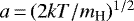
To understand the influence of small-scale inhomogeneities (clumping) on the derived parameters, we calculated an additional set of models that account for optically thin inhomogeneities (for details see Krtička et al. 2018). The clumping is parameterized by a clumping factor, which is introduced as  , and where the angle brackets denote the average over volume. The value of Cc = 1 corresponds to a smooth flow. We adopted the empirical radial clumping stratification from Najarro et al. (2009) and Bouret et al. (2012)
 (1)
(1)
where C1 is the clumping factor and the velocity C2 determines the location of the onset of clumping. We adopted C1 = 10 close to the value for which the empirical Hα mass-loss rates of O stars agree with observations (Krtička & Kubát 2017) and C2 = 100 km s−1, which is a typical value derived in Najarro et al. (2009). In Eq. (1) we insert the fit of the velocity of the unclumped wind (Cc = 1) in an improved polynomial form of Krtička & Kubát (2011) as follows:
 (2)
(2)
where vi and γ are parameters of the fit given in Table 2. We note that this formula gives a more precise fit to the radius dependence of velocity calculated by the solution of hydrodynamic equations than the commonly used β-velocity law for any β.
Stellar parameters of the model grid with derived values of the terminal velocity v∞ and the mass-loss rate Ṁ.
3 Calculated wind models
Table 1 lists the input parameters of wind models and corresponding wind parameters calculated without clumping. The wind mass-loss rate Ṁ scales mostly with the stellar luminosity. At fixed luminosity, the mass-loss rate slightly decreases with decreasing effective temperature down to about Teff = 22.5 kK (Fig. 1, see also Vink 2018). This trend can be explained by a gradual shift of the emergent flux from the ultraviolet region (where most of driving lines appear) to the visible region (Vink et al. 2000; Krtička et al. 2020). Around Teff = 20 kK the mass-loss rate increases by a factor of about 6 (Pauldrach & Puls 1990). This rise of the mass-loss rate is usually referred to as a bistability jump. It is caused by the iron recombination from Fe IV to Fe III, which accelerates wind more efficiently (Vink et al. 1999; Vink 2018). The increase of the mass-loss rate is not instantaneous, but gradual in the interval of about 5 kK.
The mass-loss rates of B supergiants and O stars from Krtička & Kubát (2017) can be simultaneously fitted via
![Mathematical equation: \begin{eqnarray*} &&\log\left({\frac{\dot M}{1\, {{M}_{\odot}\,\textrm{yr}^{-1}} }}\right)\,{=}\, a + b \log\left({\frac{L}{10^6L_{\odot}}}\right)\nonumber \\ &&\quad\quad -a \log\left\{{\exp\left[{-\frac{\left({T-T_1}\right)^2}{\Delta T_1^2}}\right] + c \exp\left[{-\frac{\left({T-T_2}\right)^2}{\Delta T_2^2}}\right]}\right\}.\end{eqnarray*}](/articles/aa/full_html/2021/03/aa39900-20/aa39900-20-eq4.png) (3)
(3)
The parameters of the fit are given in Table 3. The fit provides an approximation for predicted mass-loss rates with a typical error of about 20%.
The temperature variations of the mass-loss rate can be also described using Fig. 2, which plots the contribution of individual elements to the line radiative force and the mean ionization degree contributing to that force. For higher temperatures, Teff > 20 kK, the wind is driven mostly by lighter elements C, Si, P, and S. As the wind ionization decreases with decreasing temperature for Teff < 20 kK, iron recombines from Fe IV to Fe III and takes over most of the wind acceleration. This results in a strong increase of the mass-loss rate explaining the “bistability-jump” behavior of hot star winds (Pauldrach & Puls 1990; Vink et al. 1999).
Table 2 gives the parameters of the fit of the wind velocity via Eq. (2). In mostcases, the wind velocity is only described precisely enough by two velocity parameters, v1 and v2. The parameter γ is always close to 1. This means that the size of nearly hydrostatic photosphere, which is about (γ − 1)R*, is relatively small despite the supergiant classification of all model stars. This can also be described in terms of the ratio of the density scale height H to the stellar radius, H∕R*~ Teff∕(gR*), which scales as H∕R*~ 1∕Teff for stars at a constant luminosity. Therefore, this ratio varies roughly by a factor of about 3 for studied stars and does not exceed 0.1, as can also be seen from variation of parameter γ − 1 with temperaturein Table 2. This differs from central stars of planetary nebulae, which also evolve at constant luminosity, but which have significantly lower radii, consequently, for cool central stars of planetary nebulae the atmospheric density scale height is comparable with their radius (Krtička et al. 2020).
Wind terminal velocity v∞ is predicted to be proportional to the escape speed vesc (Castor et al. 1975b). For stars at fixed luminosity, the stellar radius increases with decreasing effective temperature. Therefore, the escape speed and wind terminal velocity become lower for cooler stars. However, the predicted relation between v∞ and vesc is more complex. The wind terminal velocity significantly decreases with temperature especially in the region around Teff = 20 kK (Vink 2018). The decrease of the wind terminal velocity in this region can be explained from the point of view of the line strength distribution function (Puls et al. 2000, see also Appendix B). With decreasing temperature, wind becomes progressively more accelerated by the iron lines (corresponding to lower α in Fig. B.1). These lines are weaker than the lines of lighter elements, many of which become optically thin in the outer wind region and therefore do not accelerate the wind so efficiently to high terminal velocities.
On average, the ratio of wind terminal velocity and escape speed can be fitted as
![Mathematical equation: \begin{equation*} \frac{v_{\infty}}{v_{\textrm{esc}}}\,{=}\, \frac{1}{2}\left[{\left({v_+-v_-}\right)\frac{t}{1+|t|}+v_++v_-}\right],\qquad t\,{=}\,\frac{T_{\textrm{eff}}-T_0}{\Delta T},\end{equation*}](/articles/aa/full_html/2021/03/aa39900-20/aa39900-20-eq5.png) (4)
(4)
where the fit parameters v+ and v− correspond to the limit of ratio at the hot and cool end of the grid, T0 corresponds to the jump temperature, and ΔT to the width of the jump. The parameters derived from the fit of our numerical results are given in Table 4.
The terminal velocity is around 100 km s−1 for many models with Teff ≲ 12.5 kK. This velocity could correspond to the slow (subcritical) solutions of line-driven wind (Castor et al. 1975b). In most models, we are able to discriminate between slow and fast solutions (see Fig. 4a in Abbott 1980) except at low effective temperatures, where the fast solution approaches the slow solution. We were unable to find the faster solutions at low temperatures, consequently, the real terminal velocities could be slightly higher.
In Fig. 3 we compare emergent fluxes calculated using our global models with fluxes derived from static plane-parallel photosphere models. These fluxes nicely agree below the Lyman jump, because this part of continuum originates in hydrostatic photosphere (Gabler et al. 1989). The fluxes in this part of spectra differ only in the atmosphereswith very low gravity, where the effect of sphericity becomes important (Kunasz et al. 1975; Gruschinske & Kudritzki 1979; Gabler et al. 1989; Kubát 1996, 1997). The fluxes from hydrostatic and global models significantly differ for frequencies higher than the Lyman jump, because at high frequencies the continuum formation region moves into the wind.
With decreasing effective temperature, the ionizing flux in general decreases. However, there are significant differences between far-ultraviolet fluxes from the static plane-parallel models and global models with winds, which can to a large extent be explained by the temperature bump appearing at low Rosseland optical depths. This bump results from the Doppler shift of line centers fromtheir static positions leading to enhanced heating of the gas (Gabler et al. 1989). Further discussion of this interesting effect is given in Puls et al. (2005). At the highest effective temperatures considered in our grid, the far-ultraviolet continuum of global models forms in the regions with lower temperature than in hydrostatic models (below the temperature bump), therefore the flux in Lyman and He I continuum is lower in global models. Around Teff≈ 20 kK the temperature bump with nearly constant temperature becomes extended and as a result the jump at 5.9 × 10¹⁵ s−1 due to He I disappears. For even lower effective temperature the continuum forms in the region of the bump, which is hotter than the corresponding region of the static plane-parallel atmosphere, consequently, the far-ultraviolet flux also becomes higher.
The difference between emergent fluxes calculated from the plane-parallel and global model atmospheres also appears in the number of ionizing photons emitted per unit of surface area,
 (5)
(5)
given in Table 5. In this equation, Hν is the Eddington flux and the ionization frequency ν0 stands for the ionization frequencies of H I, He I, and He II. While for hotter stars Teff≳ 40 kK the plane-parallel models give a reasonable estimate of number of H I and He I ionizing photons (Krtička et al. 2020), for early B supergiants the plane-parallel models overestimate the ionizing fluxes and for late B supergiants underestimate ionizing fluxes with respectto global models. At the hot end, the predicted number of ionizing photons corresponds to extrapolated results for O supergiants from Puls et al. (2005) and from Martins et al. (2005a). Our ionizing fluxes slightly differ from those derived by Smith et al. (2002) from WM-BASIC models.
Wind parameters predicted from models calculated with clumping after Eq. (1) are given in Table 2. Clumping increases the mass-loss rate because it favors recombination and ions with lower charge drive wind more efficiently (Muijres et al. 2011; Krtička et al. 2018). From the results in Table 2, the wind mass-loss rates increase with clumping on average as  . The effect of clumping is weaker than in O supergiants, in which the mass-loss rate scales with clumping as
  (Krtička et al. 2018). The lower sensitivity of the mass-loss rate to clumping is connected with the fact that radiative force in the range 22.5−27.5 kK is typically dominated by single ionization state for most elements, therefore clumping does not significantly vary the redistribution of the force among individual ionization states. On the other hand, with clumping the increase of mass-loss rate resulting from iron recombination appears at higher effective temperatures because the clumping shifts the onset of the recombination from Fe IV to Fe III.
We further tested the influence of C2 parameter in Eq. (1) to understand whether a weaker sensitivity to clumping is connected with the value of this parameter, which determines the position of the onset of clumping. The tests showed that this is not the case. For most models, a lower parameter C2 = 30 km s−1 leads just to a slight increase of the wind mass-loss rate.
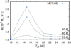 |
Fig. 1 Mass-loss rates Ṁ without clumping predicted by our models as a function of the stellar effective temperature Teff. |
 |
Fig. 2 Relative contribution of individual elements to the line radiative force at the wind critical point. Plotted as a function of the stellar effective temperature for models with M = 40 M⊙. The thick blue line plots the mean ionization state that contributes to the line radiative force. This is defined as ∑fizi∕(∑fi), where zi is the ionization state of ion i and fi is its contribution to the line radiative force. This plot was derived in a simplified way using the Sobolev approximation. |
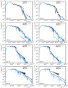 |
Fig. 3 Comparison of the emergent fluxes from the plane-parallel TLUSTY (black line) and global METUJE (blue line) models smoothed by a Gaussian filter. Stellar wind modifies the flux mostly above the Lyman jump. Plotted for selected models fromTable 1 (denoted in the plots). |
Calculated number of ionizing photons per unit of surface area  .
.
4 Comparison with observations and other theoretical models
The test of predicted wind mass-loss rates against the observations is not straightforward owing to the effect of clumping on the observational wind indicators. Small-scale wind inhomogeneities (clumping) are expected as a consequence of strong radiatively driven wind instability (Owocki et al. 1988; Feldmeier et al. 1997; Feldmeier & Thomas 2017). Clumping shifts the ionization equilibrium (Hamann & Koesterke 1998; Bouret et al. 2003; Martins et al. 2005b; Puls et al. 2006) as a result of stronger recombination in overdense regions. This affects the classical wind mass-loss rate indicators such as Hα line, ultraviolet wind lines, and infrared and radio excess. The inferred values of wind mass-loss rates spoiled by stronger recombination can be corrected for clumping by multiplication by the factor of  . However, this simple scaling breaks down in the case of clumps that are optically thick either in continuum (Feldmeier et al. 2003)or in lines (Oskinova et al. 2007; Sundqvist et al. 2010, 2011; Šurlan et al. 2012, 2013).
Figure 4 compares predicted mass-loss rates with results derived from Balmer lines and mass-loss rates from radio data. None of these observational estimates account for clumping. For stars with Teff> 20 kK, the observational results are roughly by a factor of 9 higher than the predicted values. Assuming that the observational results should be scaled down by a factor of  and that the predicted result increase by a factor of
  , the observational and predicted values would agree for a higher value of Cc than we used in our models, namely Cc = 24.
For stars with Teff < 20 kK, the agreement between the observational and predicted mass-loss rates is better (Fig. 4). Although there is a group of stars that show mass-loss rates significantly above the theoretical predictions, the ratio of observational and theoretical mass-loss rates decreases as a function of effective temperature and approaches 1 around the mass-loss rate maximum at about Teff = 15 kK. This implies that a lower clumping factor of Cc = 5 (on average) is required to bring observations and theory to agreement. This conclusion agrees with the results derived from the CMFGEN code (Petrov et al. 2014), according to which the Hα line is only weakly sensitive to (optically thin) clumping for cool B supergiants. Therefore, the Hα mass-loss rates should be close to the theoretical expectations.
Besides determinations that are sensitive to clumping, there are methods that yield mass-loss rates that are either independent of clumping or can be corrected for clumping. Such rates are plotted in Fig. 5. We plot the mass-loss rate (for ϵ Ori) derived from X-ray line profiles (Puebla et al. 2016), which is independent of the effect of optically thin clumps, but may be affected by optically thick inhomogeneities (Feldmeier et al. 2003). Figure 5 also includes mass-loss rates of B supergiant components of high-mass X-ray binaries determined from UV line profiles corrected for optically thin clumps (Hainich et al. 2020)and mass-loss rates of B supergiants derived from stellar bow shocks (Kobulnicky et al. 2019). On average, these observational estimates are by a factor of 1.4 higher than our predictions (disregarding a star with Teff = 20 kK). Therefore, the observational mass-loss rates that are not affected by clumping agree much better with our predictions, although significant discrepancies exist even here.
Figures 4 and 5 also compare our results with predictions of Vink et al. (2001), Petrov et al. (2016), and Björklund et al. (2020). From Fig. 4 it follows that our predicted mass-loss rates are significantly lower than predictions of Vink et al. (2001) by a factor of 13 and 8 for the models with Teff> 20 kK and Teff< 20 kK, respectively.This difference can be attributed to the effect of line overlaps and to the Sobolev approximation used by Vink et al. (2001) to calculate the line force (Krtička & Kubát 2017). The latter is demonstrated in Fig. 6, where we plot the ratio of CMF and Sobolev line forces as a function of velocity. This ratio is close to 1 for velocities on the order of a few thermal speeds, which means that the Sobolev approximation is valid in that case. However, the ratio shows a deep minimum around vr ≈ 0.1a (a is a hydrogen thermal speed) owing to a positive source function gradient near the photosphere (Krtička & Kubát 2010).
In Fig. 5 we also overplot mass-loss rates predicted using modified CMFGEN models (Petrov et al. 2016). These models adopt similar assumptions as our code. Their results nicely agree with our predictions with an exception of the regions around Teff≈ 20 kK, where Petrov et al. (2016) predict significantly larger mass-loss rates possibly due to evolutionally earlier (i.e., for higher temperatures) onset of iron recombination connected with the inclusion of clumping. Björklund et al. (2020) predict mass-loss rates from the global version of the FASTWIND code with CMF line force. Their model assumptions are very similar to ours, however their models were calculated for O stars. Still, there is a near overlap of the grids around Teff≈ 28 kK, where the predictions reasonably agree.
Clumps may directly affect the radiative transfer when they become optically thick (termed porosity and vorosity). This leads to an effectively gray opacity of clumped media and an underestimation of mass-loss rates derived from ultraviolet P Cygni line profiles (Oskinova et al. 2007; Sundqvist et al. 2011; Šurlan et al. 2013). Therefore, ratio of wind strengths of resonance doublet components can be used to test the effect of clumping (Prinja & Massa 2010). If the ratio is close to the ratio of oscillator strengths, then the porosity is negligible, while when it is equal to 1, then the porosity is significant.
Prinja & Massa (2013) applied this method to narrow absorption components, which appear close to the blue edge of P Cygni line profiles due to accumulation of discrete absorption components. These authors concluded that these narrow absorption components are not affected by porosity in B supergiants and, consequently, are suitable for the mass-loss rate determination and they estimated the product of ionization fraction and mass-loss rate for studied stars, q(Si IV)Ṁ. In Fig. 7 we plot these values for the stars for which we derived luminosities either from the literature (Kudritzki et al. 1999; Crowther et al. 2006; Lefever et al. 2007; Haucke et al. 2018) or determined using absolute magnitudes from Kaltcheva et al. (2020) and bolometric corrections of Crowther et al. (2006). The observational values are plotted relative to the predicted mass-loss rate Ṁ and compared to predicted ionization fractions. The observational values of q(Si IV)Ṁ are significantly lower than predictions for stars at the hot side of the studied region, where Si IV is a dominant ionization stage. With decreasing effective temperature, silicon recombines from Si IV to Si III, improving the agreement between observations and theory for lower effective temperatures. The recombination is stronger with clumping, which explains the better agreement between the theory and observations in Fig. 7 with clumping in some cases. The huge disagreement at the high effective temperatures is most likely caused by X-rays, which significantly affect the Si IV ionization fraction (Krtička & Kubát 2009; Carneiro et al. 2016). Moreover, the radiative transfer in corotating interaction regions, where the narrow absorption components are supposed to originate (Cranmer & Owocki 1996; Lobel & Blomme 2008; David-Uraz et al. 2017), is complex. Another problem is that only a small fraction of mass-loss is carried by corotating interacting regions.
The models are able to reasonably reproduce the wind terminal velocity. The wind terminal velocity is proportional to the escape speed (Castor et al. 1975b), therefore the ratio of these velocities does not show strong variations as a function of effective temperature. In Fig. 8 we compare the predicted ratio of the terminal velocity and escape speed with values derived from observations. The ratio decreases from about 3 to 1 as a result of bistability jump, which agrees with observations (Lamers et al. 1995; Crowther et al. 2006) and theoretical calculations (Vink 2018).
To some extent, our models are also able predict the observed spectra (see Fig. 9). The extent of the absorption part of the P Cygni line profiles is reasonably reproduced. This means that our models provide a reliable estimate of the terminalvelocities. While the Si IV doublet is also typically reproduced well, the C IV doublet is too weak for cooler stars. We note that the comparison of individual observed spectra is done using our limited grid of models and we do not aim for a detailed analysis of individual objects.
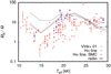 |
Fig. 4 Ratio of published mass-loss rates derived from observations using analysis that neglects clumping (Ṁlit), and mass-loss rates predicted using Eq. (3), plotted as a function of effective temperature Teff for B supergiants. The observations include Balmer line (mostly Hα) mass-loss rates of Galactic B supergiants (Kudritzki et al. 1999; Crowther et al. 2006; Lefever et al. 2007; Markova & Puls 2008; Haucke et al. 2018, red plus symbols), Hα mass-loss rates of B supergiants from the Small Magellanic Cloud (Evans et al. 2004; Trundle et al. 2004; Trundle & Lennon 2005, red triangles) scaled according to Ṁ ~ Z0.59 (Krtička& Kubát 2018), and mass-loss rates from radio data (Scuderi et al. 1998; Benaglia et al. 2007, violet squares). The ratios of the predictions of Vink et al. (2001) to our predictions for three different luminosities are overplotted (solid gray lines). Plotted with v∕vesc = 2 for Teff ≥ 20 kK and with v∕vesc = 1.3 for Teff ≤ 20 kK. |
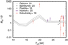 |
Fig. 5 Ratio of observational (Ṁlit) and predicted (Ṁ) mass-loss rates as a function of effective temperature Teff for B supergiants. Only observational mass-loss rates that are either independent of clumping or were corrected for clumping in some way are plotted. The observational results are based on X-ray line profiles (Puebla et al. 2016), UV spectrum analysis with clumping (Hainich et al. 2020), and wind bow shocks (Kobulnicky et al. 2019). The gray lines denote predictions of Petrov et al. (2016) for different luminosities and masses and the gray squares correspond to predictions of Björklund et al. (2020) and Teff = 27 500 K. |
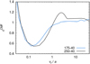 |
Fig. 6 Ratio of CMF line force and line force calculated using the Sobolev approximation (denoted ad
cCMF) as a function of velocity evaluated in terms of the depth dependent hydrogen thermal speed
|
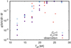 |
Fig. 7 Comparison of calculated and observed (Prinja & Massa 2013) Si IV ionization fractions. The observed product of the Si IV ionization fraction and mass-loss rate q(Si IV)Ṁ was divided by the predicted mass-loss rate to obtain the Si IV ionization fraction. The calculated ionization fractions are plotted with (Cc = 10) and without (Cc = 1) clumping forv = 0.9 v∞. |
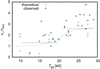 |
Fig. 8 Comparison of calculated and observed (Crowther et al. 2006) ratios of the wind terminal velocity and surface escape velocity. The dashed lines denote a mean relationship of Lamers et al. (1995) and the dotted blue line denotes mean predicted ratio according to Eq. (4). |
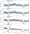 |
Fig. 9 Comparison of theoretical spectra from our grid and observed spectra of selected B supergiants. The observed IUE spectra of HD 198478 (SWP 6335), HD 41117 (SWP 6338), HD 2905 (SWP 1814), and HD 37128 (SWP 8130) are plotted. |
5 Discussion
5.1 Limitations of the models
There are several limitations of our models that may affect the final results. The most obvious limitation is the insufficiently accurate treatment of small-scale wind structures, which are typically nicknamed as the effect of clumping. Table 2demonstrates that optically thin inhomogeneities increase the predicted mass-loss rates, while the optically thick inhomogeneities may have the opposite effect, as described by Muijres et al. (2011).
For our modeling, we only account for elements with the highest abundances, while other elements are neglected (see Krtička et al. 2020, for the list). This is likely not a problem for lighter elements such as Cl or K, which do not significantly contribute to the radiative force (Sander et al. 2017). Iron-peak elements could possibly contribute to the radiative force more significantly as a result of their higher number of lines, but these elements typically have at least two orders of magnitude lower abundance than iron and nickel, which are included in our models.
A potentially more significant problem may come from the number of lines that are accounted for. Our line list is mostly based on observed lines, while theoretical calculations give much higher number of lines (Kurucz 2018). This is not a problem for lighter elements, for which the line list was updated to include even lines that are not observed. However, for iron the theoretical line list includes a number of lines that is two orders of magnitude larger than our line list, which may give rise to a larger error of the line force. To test this, we compared line force calculated with shorter and longer iron line list and the difference was typically just few percent. Slightly larger differences appeared in the photospheric region, thus possibly affecting the structure of the photosphere slightly, but not the mass-loss rate. Consequently, accounting for the longer line list does not significantly affect our results.
5.2 Bistability region
Theoretical models agree in the prediction of a jump in wind mass-loss rates (Pauldrach & Puls 1990; Vink et al. 1999; Petrov et al. 2016) and terminal velocities (Vink 2018) around Teff ≈ 21 kK. This is called the bistability jump. Each of these models applied different approximations to determine the quantities characterizing the bistability jump, namely mass-loss rates and terminal velocities, and yet derive comparable results. Pauldrach & Puls (1990, who discovered the existence of the jump) used force multipliers to determine the radiation force. Vink et al. (1999) combined several codes and succeeded in obtaining significantly improved values of predicted mass-loss rates, and Petrov et al. (2016) additionally used the code CMFGEN with CMF radiative transfer. However, the observational support for the bistability jump is less clear. While the gradual decrease of terminal velocities in the bistability region (a region of effective temperatures where the bistability jump appears) is clearly supported by observations (see Fig. 8, Lamers et al. 1995; Crowther et al. 2006), the presence of a jump in mass-loss rates is unclear (Crowther et al. 2006). There is an indication of a presence of a jump in radio wind efficiencies (Benaglia et al. 2007). The variability of the mass-loss rates of luminous blue variables during their variation cycles of S Doradus type can be described using varying mass-loss rates in the bistability region (Vink & de Koter 2002; Groh et al. 2011).
Our models are able to reproduce the observational behavior of mass-loss rates provided that the clumping factor decreases from about 24 at the hot side of the jump to about 5 at its cool side. Stronger clumping (higher clumping factor) at the hot side of the bistability region can be connected with decrease of macroturbulent velocity with decreasing effective temperature detected by Dufton et al. (2006) and Markova & Puls (2008). At the cool side of the bistability region, the difference between predicted and observational mass-loss rates decreases with effective temperature. The wind terminal velocity also decreases with decreasing effective temperature, possibly decreasing the amount of clumping and as a result moderating the effect of clumping on observational values (Driessen et al. 2019).
Theoretical models predict that the Hα line becomes optically thick for cool B supergiants, leading to the appearance of the classical P Cygni line profile (Petrov et al. 2014). Therefore, the line may become sensitive to optically thick clumping. This could mean that observational Hα mass-loss rate determinations are underestimated at the cool side of the bistability jump because the lines become optically thick there (Sundqvist et al. 2011; Šurlan et al. 2013).
5.3 Evolutionary implications
Massive stars lose a significant fraction of their mass during the evolutionary phases corresponding to luminous B stars. For example, evolutionarymodels (employing Vink et al. 2001 mass-loss rates) predict that a solar-metallicity star with an initial mass of 60 M⊙ loses about 25 M⊙ during the evolutionarystage of B supergiants (Groh et al. 2014). On the other hand, our models were calculated for relatively low values of the Eddington parameter Γ ≈ 0.2−0.3 (see Table 1). When the star becomes a luminous blue variable, it approaches the Eddington limit and its mass-loss rate significantly increases (Gräfener et al. 2011; Vink 2018). To maintain a large total amount of mass lost during stellar evolution, ehnanced mass loss close to the Eddington limit can possibly compensate for lower values of mass-loss rates predicted in this work. Moreover, stars in a proximity of the Eddington limit may have a strong porous optically thick outflow (Shaviv 1998; Owocki et al. 2004) or may experience explosive mass-loss events (Owocki et al. 2019).
Stars with a lower initial mass (≲30 M⊙) do not lose a significant fraction of their mass as a result of line-driven winds (Renzo et al. 2017). Consequently, the reduction of mass-loss rates mentioned in this work might not be significant for the evolution of these stars. On the other hand, the compactness of the core of pre-supernova models is sensitive to mass-loss during the hot evolutionary phase (Renzo et al. 2017). Compactness is one of the parameters that determines an outcome of a supernova explosion (O’Connor & Ott 2011; Ugliano et al. 2012).
Stars donot only lose mass via their winds, but also angular momentum. Vink et al. (2010) proposed that low observed rotational velocities of cool B supergiants could be caused by stronger angular momentum loss in the vicinity of the bistability jump. Keszthelyi et al. (2017) tested several experimental wind prescriptions and concluded that low rotational velocities of cool B supergiants could be reproduced even with weaker mass-loss rates, but with a bistability jump in mass-loss rates.
In the early evolutionary phases the wind velocity slows down with decreasing effective temperature and while the star passes the bistability region, the mass-loss rate increases. In later evolutionary phases, for example during the Wolf-Rayet phase, the wind velocity increases again. Consequently, the faster wind in later evolutionary phases may collide with the wind from earlier evolutionary phases and create circumstellar structures similar to those found in planetary nebulae (Kwok et al. 1978).
5.4 Domains of radiatively driven mass loss
Abbott (1979) introduces two limits (static and wind limit, see his Fig. 1) and discriminates between three zones in the Hertzsprung-Russell diagram. Above the static limit, fully hydrostatic photospheres are not possible, the radiative force overcomes gravity at some point, and the wind is self-initiated. Below the static limit and above the wind limit, hydrostatic photospheres are possible, therefore the wind is not self-initiated, but it can be sustained. Therefore, two types of solutions exist in this region. Below the wind limit, only hydrostatic photospheres are possible and the chemically homogeneous wind does not exist.
To plot these wind domains in Fig. 10, we used the spectroscopic Hertzsprung-Russell diagram (Langer & Kudritzki 2014; Castro et al. 2014) and overplotted the results of models from OSTAR2002 and BSTAR2006 static model atmosphere grids (Lanz & Hubeny 2003, 2007). For high luminosities, static atmospheres are not possible, and the outer atmospheric levels expand triggering the wind. This case corresponds to the atmospheres of B supergiants. However, for many B supergiants the radiative force grad exceeds the magnitude of gravity g only in single outermost layer of the model atmosphere. This layer may be the subject of numerical inconsistencies, consequently, many B supergiants may lie close to the static limit.
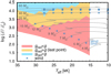 |
Fig. 10 Domains of radiatively driven mass loss in the spectroscopic Hertzsprung-Russell diagram. The domains were derived from the balance of gravity and radiative force using the OSTAR2002 and BSTAR2006 static model atmosphere grids (Lanz & Hubeny 2003, 2007, respectively). In this diagram,
|

5.5 X-ray emission
Hot stars emit X-rays, which in most cases originate in shocks thought to be caused by line driven wind instability (Owocki et al. 1988; Feldmeier et al. 1997). In B supergiants, the X-ray emission typically appears only in the earliest spectral types up to about B3 (Berghoefer et al. 1997; Nazé 2009). This roughly corresponds to the effective temperature of about 15 kK (Markova & Puls 2008).
The wind X-ray emission is powered by the wind kinetic energy. In Fig. 11 we plot the wind power  as a function of the effective temperature. The wind power does not significantly vary in hotter B supergiants even in the region of recombination of Fe IV to Fe III, where the increase of the mass-loss rate is compensated by the decrease of the wind terminal velocity. On the other hand, mostly as a result of a decrease of the wind terminal velocity, the wind power significantly decreases between 17.5–12.5 kK, exactly in the region where the X-ray emission disappears.
The temperature of the post-shock gas is proportional to the square of the terminal velocity. As a result, with decreasing effective temperature the post-shock gas temperature significantly decreases (Fig. 11) from about 5 MK for Teff = 17.5 kK to about 200 kK for Teff = 12.5 kK (using velocities from Table 1 and Eq. (1) of Owocki et al. 2013). Therefore, the X-ray emission becomes negligible at such low temperatures (e.g., Raymond & Smith 1977; Landini & Monsignori Fossi 1984).
Depending on the dominant cooling mechanism, shocks may be either radiative or adiabatic. As a result of the decrease of the wind density with radius, shocks are typically radiative close to the star and adiabatic in the outer wind parts. Because of their large stellar radii, from Eq. (24) of Owocki et al. (2013) it follows that the transition from radiative to adiabatic shocks appears in B supergiants relatively close to the star at a typical distance of few stellar radii.
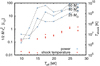 |
Fig. 11 Wind power (left axis) and shock temperature (right axis) as functions of stellar effective temperature. |
5.6 Influence of the magnetic field
Although the Zeeman splitting does not directly affect the wind mass-loss rate for typical magnetic fields detected in OB stars (Krtička 2018), the magnetic field still affects the mass-loss rate as a result of wind channelling along the field lines (ud-Doula & Owocki 2002). The effect of the magnetic field scales with the ratio of the magnetic field energy density to the wind kinetic energy density, which at large distances from the star simplifies to the wind magnetic confinement parameter of ud-Doula & Owocki (2002)
 (6)
(6)
where Beq is the equatorial field strength. For weak confinement, η*≲ 1, the magnetic field opens up and the wind flows radially. On the contrary, for strong confinement, η* ≳ 1, the wind is trapped by the magnetic field.
In rewriting Eq. (6) in terms of typical parameters of B supergiants, we derive
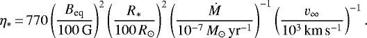 (7)
(7)
The field strength in typical magnetic O stars is on the order of 1 kG (Donati et al. 2006; Wade et al. 2012). Assuming flux conservation, which is approximately valid in more massive magnetic chemically peculiar stars (Landstreet et al. 2007), the magnetic field strength in B supergiants is on the order of 10 G. This is a typical strength of magnetic fields found in evolved BA stars (Fossati et al. 2015; Neiner et al. 2017; Martin et al. 2018). From Eq. (7), it follows that such fields are able to strongly confine the stellar wind.
The angular momentum loss from magnetized wind leads to rotational braking. In principle, this could provide additional angular momentum loss required by evolutionary models with low mass-loss rates to reproduce observed rotational velocities (Keszthelyi et al. 2017). With an angular momentum constant k on the order of 0.01 as derived from MESA evolutionary code (Paxton et al. 2011, 2013) for a B supergiant stage of the star with initial mass 40 M⊙, the magnetic braking timescale is on the order of 1 Myr using Eq. (25) of Ud-Doula et al. (2009) and typical wind parameters found in this work. This is order of magnitude longer than the duration of B supergiant stage (Groh et al. 2014). From this it follows that the magnetic braking does not likely significantly affect the rotational speed of B supergiants.
5.7 Pure absorption models
Analyzing the topology of wind solutions around the sonic point, Poe et al. (1990) concluded that pure absorption models have nodal topology instead of the saddle-type topology, which would correspond to solar wind. This leads to a strong instability of time-dependent pure absorption wind models (Owocki et al. 1988) and may prevent us from calculating time independent models. However, the line emission may restore the saddle-type topology and provide stability for time independent models (Sundqvist & Owocki 2015).
To test this, we recalculated the wind model 275-60 neglecting line emission in CMF radiative transfer equation and starting with a converged model corresponding to a relatively low mass-loss rate. It turned out that we were unable to converge the pure absorption model. Therefore, the inclusion of the line emission (scattering) is crucial to obtain well-converged wind models. We further tested the solution topology around the sonic point, thereby concluding that the wind has a saddle-type topology in the case with emission, but a nodal topology without emission (see Appendix A).
6 Conclusions
We provide global line-driven wind models for B supergiants at the metallicity corresponding to our Galaxy. The structure of the flow is determined consistently from the nearly hydrostatic photosphere to the wind expanding with supersonic speed. The winds are driven mostly by C, Si, and S for hotter B supergiants, while iron dominates wind driving in cooler supergiants. We determined basic wind parameters, that is, the mass-loss rates and terminal velocities.
We generalized our formula for fast estimates of mass-loss rate predictions of O stars to B supergiants as well (Eq. (3)). The mass-loss rate depends mostly on the stellar luminosity. The dependence of the mass-loss rate on the effective temperature is nonmonotonic. The mass-loss rates decrease with temperature down to a minimum at about 22.5 kK. For cooler stars the mass-loss rates gradually increase by a factor of about 6 in the region of bistability. The increase is caused by recombination of iron from Fe IV to Fe III. The mass-loss rates reach maximum at about 15 kK, where they start to decrease with temperature again.
The wind terminal velocity is proportional to the escape speed for a given effective temperature, as can be seen from our fitting formula Eq. (4). The ratio of the terminal velocity to the escape speed decreases from about 2–3 at the hot side of the region of iron recombination to about 0.5–1.5 at the cool side. This nicely agrees with observations.
The comparison with mass-loss rates derived from observations is more problematic as a result of the effect of clumping on the observational indicators. The mass-loss rates that are uncorrected for clumping are by a factor of 3 higher than the predictions on the cool side of the bistability, while they are by a factor of 9 higher than the predictions at the hot side of the bistability. These differences can be alleviated by the influence of clumping on observational determinations and on the predictions. Hence clumping that decreases with temperature can resolve the discrepancy between mass-loss rate estimates affected by clumping and theoretical predictions (Driessen et al. 2019). On the other hand, the mass-loss rate estimates that are not sensitive to clumping reasonably agree with our predictions. Mass-loss rates derived from X-ray line profiles, UV spectroscopy that accounts from clumping, and stellar bow shocks are on average just by a factor of 1.4 higher than our predictions.
The predicted mass-loss rates are by a factor of about 10 lower than values being used in current evolutionary models. Together with previous studies that predict a similar reduction of line-driven mass-loss rates (Krtička & Kubát 2017; Sundqvist et al. 2019), this result calls for a re-evaluation of the role of winds in evolution of massive stars.
Acknowledgements
This work was supported by grant GA ČR 18-05665S. Computational resources were supplied by the project “e-Infrastruktura CZ” (e-INFRA LM2018140) provided within the program Projects of Large Research, Development and Innovations Infrastructures. The Astronomical Institute Ondřejov is supported by a project RVO:67985815 of the Academy of Sciences of the Czech Republic.
Appendix A Solution topology around the sonic point
As shown by Holzer (1977), the solution topology can be determined from the analysis of the momentum equation
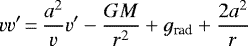 (A.1)
(A.1)
around the sonic point. In this equation, we neglected the radial variations of the isothermal sound speed a, grad denotes the radiative force, and  . The momentum equation Eq. (A.1) yields for the velocity gradient
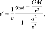 (A.2)
(A.2)
where we dropped the last term on the right-hand side of Eq. (A.1), which is negligible for line-driven winds. At the sonic point, the velocity derivative is derived using the L’Hospital’s rule, which gives
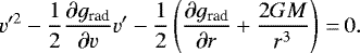 (A.3)
(A.3)
We assumed that grad is a function of radius and velocity only. Close to the sonic point the derivative of the radiative force dominates in the last bracket in Eq. (A.3), hence Eq. (A.3) has positive and negative roots implying a saddle-type topology if
 (A.4)
(A.4)
as was derived by Poe et al. (1990).
It is difficult to derive ∂grad∕∂r directly from numerical models. However, the models give dgrad∕dr from the radial dependence of the radiative force, which can be converted to the partial derivative using
 (A.5)
(A.5)
The derivative ∂grad∕∂v can be computed numerically from two runs with slightly different velocity. We tested the solution topology in the wind models with line emission using Eq. (A.4). The partial derivative in Eq. (A.4) is positive implying saddle topology around the sonic point, as already shown from analytic calculations by Sundqvist & Owocki (2015). We note that this holds even if the critical point of our wind models appears downstream at the point where the wind velocity is equal to the speed of radiative-accoustic waves (Abbott 1980; Thomas & Feldmeier 2016).
Appendix B Line strength distribution functions
The contribution of lines with different strengths to the radiative force can be described using the line strength distribution function (Castor et al. 1975b; Puls et al. 2000). The line strength distribution function can be conveniently parameterized using k, α, and δ parameters, which enable the simplification of the calculation of the line force. Puls et al. (2000) showed that the α parameter corresponds to the ratio of radiative force due to optically thick lines to the total line force.
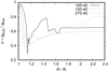 |
Fig. B.1 Ratio of the radiative force due to the optically thick lines to the total line force as a function of radius. The division between optically thick and optically thin lines was selected at the unity radial Sobolev optical depth. The figure was plotted for three selected models. The optical depths and the line force were calculated in the Sobolev approximation. |
Both optically thick and optically thin lines contribute to the radiative driving. This is illustrated in Fig. B.1, where we plot the ratio of the optically thick line force to the total line force. This ratio also corresponds to the α parameter and it should be constant for line strength distribution function with uniform shape. This is true in some parts of the figure for the low-density 100-40 model. However, the ratio significantly varies with radius for higher density model 150-40 as a result of curvature of line strength distribution function. The line driving is dominated by optically thick lines close to the star (for low velocities). The density decreases with increasing velocity, thereby reducing the number of optically thick lines. As a result, optically thin lines become more important at larger radii. Abrupt changes of the ratio appear owing to the change of the line strength from optically thick to optically thin for the unity optical depth. There are more optically thick lines in the model 150-40 (mostly of iron), consequently the variations are smoother in this model.
References
- Abbott, D. C. 1979, IAU Symp., 83, 237 [Google Scholar]
- Abbott, D. C. 1980, ApJ, 242, 1183 [Google Scholar]
- Abbott, D. C., & Hummer, D. G. 1985, ApJ, 294, 286 [Google Scholar]
- Abbott, B. P., Abbott, R., Abbott, T. D., et al. 2016, ApJ, 818, L22 [Google Scholar]
- Asplund, M., Grevesse, N., Sauval, A. J., & Scott, P. 2009, ARA&A, 47, 481 [NASA ADS] [CrossRef] [Google Scholar]
- Benaglia, P., Vink, J. S., Martí, J., et al. 2007, A&A, 467, 1265 [NASA ADS] [CrossRef] [EDP Sciences] [Google Scholar]
- Berghoefer, T. W., Schmitt, J. H. M. M., Danner, R., & Cassinelli, J. P. 1997, A&A, 322, 167 [Google Scholar]
- Björklund, R., Sundqvist, J. O., Puls, J., & Najarro, F. 2020, A&A, accepted [arXiv:2008.06066] [Google Scholar]
- Bouret, J.-C., Lanz, T., Hillier, D. J., et al. 2003, ApJ, 595, 1182 [Google Scholar]
- Bouret, J.-C., Hillier, D. J., Lanz, T., & Fullerton, A. W. 2012, A&A, 544, A67 [Google Scholar]
- Carneiro, L. P., Puls, J., Sundqvist, J. O., & Hoffmann, T. L. 2016, A&A, 590, A88 [NASA ADS] [CrossRef] [EDP Sciences] [Google Scholar]
- Castor, J., McCray, R., & Weaver, R. 1975a, ApJ, 200, L107 [Google Scholar]
- Castor, J. I., Abbott, D. C., & Klein, R. I. 1975b, ApJ, 195, 157 [NASA ADS] [CrossRef] [Google Scholar]
- Castro, N., Fossati, L., Langer, N., et al. 2014, A&A, 570, L13 [NASA ADS] [CrossRef] [EDP Sciences] [Google Scholar]
- Cohen, D. H., Wollman, E. E., Leutenegger, M. A., et al. 2014, MNRAS, 439, 908 [Google Scholar]
- Cranmer, S. R., & Owocki, S. P. 1996, ApJ, 462, 469 [Google Scholar]
- Crowther, P. A., Lennon, D. J., & Walborn, N. R. 2006, A&A, 446, 279 [NASA ADS] [CrossRef] [EDP Sciences] [Google Scholar]
- David-Uraz, A., Owocki, S. P., Wade, G. A., Sundqvist, J. O., & Kee, N. D. 2017, MNRAS, 470, 3672 [Google Scholar]
- Donati, J. F., Howarth, I. D., Bouret, J. C., et al. 2006, MNRAS, 365, L6 [Google Scholar]
- Driessen, F. A., Sundqvist, J. O., & Kee, N. D. 2019, A&A, 631, A172 [NASA ADS] [CrossRef] [EDP Sciences] [Google Scholar]
- Dufton, P. L., Ryans, R. S. I., Simón-Díaz, S., Trundle, C., & Lennon, D. J. 2006, A&A, 451, 603 [NASA ADS] [CrossRef] [EDP Sciences] [Google Scholar]
- Eddington, A. S. 1921, Z. Phys., 7, 351 [Google Scholar]
- Ekström, S., Georgy, C., Eggenberger, P., et al. 2012, A&A, 537, A146 [NASA ADS] [CrossRef] [EDP Sciences] [Google Scholar]
- Evans, C. J., Crowther, P. A., Fullerton, A. W., & Hillier, D. J. 2004, ApJ, 610, 1021 [Google Scholar]
- Feldmeier, A., & Thomas, T. 2017, MNRAS, 469, 3102 [Google Scholar]
- Feldmeier, A., Puls, J., & Pauldrach, A. W. A. 1997, A&A, 322, 878 [NASA ADS] [Google Scholar]
- Feldmeier, A., Oskinova, L., & Hamann, W.-R. 2003, A&A, 403, 217 [NASA ADS] [CrossRef] [EDP Sciences] [Google Scholar]
- Fossati, L., Castro, N., Morel, T., et al. 2015, A&A, 574, A20 [NASA ADS] [CrossRef] [EDP Sciences] [Google Scholar]
- Gabler, R., Gabler, A., Kudritzki, R. P., Puls, J., & Pauldrach, A. 1989, A&A, 226, 162 [NASA ADS] [Google Scholar]
- Gräfener, G.,& Hamann, W.-R. 2008, A&A, 482, 945 [NASA ADS] [CrossRef] [EDP Sciences] [Google Scholar]
- Gräfener, G., Vink, J. S., de Koter, A., & Langer, N. 2011, A&A, 535, A56 [NASA ADS] [CrossRef] [EDP Sciences] [Google Scholar]
- Groh, J. H., Hillier, D. J., & Damineli, A. 2011, ApJ, 736, 46 [Google Scholar]
- Groh, J. H., Meynet, G., Georgy, C., & Ekström, S. 2013, A&A, 558, A131 [NASA ADS] [CrossRef] [EDP Sciences] [Google Scholar]
- Groh, J. H., Meynet, G., Ekström, S., & Georgy, C. 2014, A&A, 564, A30 [NASA ADS] [CrossRef] [EDP Sciences] [Google Scholar]
- Gruschinske, J., & Kudritzki, R. P. 1979, A&A, 77, 341 [Google Scholar]
- Hainich, R., Oskinova, L. M., Torrejón, J. M., et al. 2020, A&A, 634, A49 [Google Scholar]
- Hamann, W. R., & Koesterke, L. 1998, A&A, 335, 1003 [Google Scholar]
- Haucke, M., Cidale, L. S., Venero, R. O. J., et al. 2018, A&A, 614, A91 [NASA ADS] [CrossRef] [EDP Sciences] [Google Scholar]
- Henney, W. J., & Arthur, S. J. 2019, MNRAS, 489, 2142 [Google Scholar]
- Holzer, T. E. 1977, J. Geophys. Res., 82, 23 [Google Scholar]
- Hubeny, I., & Mihalas, D. 2014, Theory of Stellar Atmospheres (Princeton: Princeton University Press) [Google Scholar]
- Hummer, D. G., Berrington, K. A., Eissner, W., et al. 1993, A&A, 279, 298 [NASA ADS] [Google Scholar]
- Kaltcheva, N., Paunzen, E., Prišegen, M., Golev, V., & Watson, M. 2020, PASP, 132, 074203 [Google Scholar]
- Keszthelyi, Z., Puls, J., & Wade, G. A. 2017, A&A, 598, A4 [NASA ADS] [CrossRef] [EDP Sciences] [Google Scholar]
- Klein, R. I., & Castor, J. I. 1978, ApJ, 220, 902 [Google Scholar]
- Kobulnicky, H. A., Chick, W. T., & Povich, M. S. 2019, AJ, 158, 73 [Google Scholar]
- Krtička, J. 2014, A&A, 564, A70 [NASA ADS] [CrossRef] [EDP Sciences] [Google Scholar]
- Krtička, J. 2018, A&A, 620, A176 [NASA ADS] [CrossRef] [EDP Sciences] [Google Scholar]
- Krtička, J., & Kubát, J. 2009, MNRAS, 394, 2065 [NASA ADS] [CrossRef] [Google Scholar]
- Krtička, J., & Kubát, J. 2010, A&A, 519, A50 [NASA ADS] [CrossRef] [EDP Sciences] [Google Scholar]
- Krtička, J., & Kubát, J. 2011, A&A, 534, A97 [NASA ADS] [CrossRef] [EDP Sciences] [Google Scholar]
- Krtička, J., & Kubát, J. 2017, A&A, 606, A31 [NASA ADS] [CrossRef] [EDP Sciences] [Google Scholar]
- Krtička, J., & Kubát, J. 2018, A&A, 612, A20 [NASA ADS] [CrossRef] [EDP Sciences] [Google Scholar]
- Krtička, J., Kubát, J., & Krtičková, I. 2018, A&A, 620, A150 [NASA ADS] [CrossRef] [EDP Sciences] [Google Scholar]
- Krtička, J., Kubát, J., & Krtičková, I. 2020, A&A, 635, A173 [CrossRef] [EDP Sciences] [Google Scholar]
- Kubát, J. 1996, A&A, 305, 255 [NASA ADS] [Google Scholar]
- Kubát, J. 1997, A&A, 323, 524 [NASA ADS] [Google Scholar]
- Kubát, J., Puls, J., & Pauldrach, A. W. A. 1999, A&A, 341, 587 [NASA ADS] [Google Scholar]
- Kudritzki, R. P., Puls, J., Lennon, D. J., et al. 1999, A&A, 350, 970 [Google Scholar]
- Kunasz, P. B., Hummer, D. G., & Mihalas, D. 1975, ApJ, 202, 92 [Google Scholar]
- Kurucz, R. L. 2018, ASP Conf. Ser., 515, 47 [NASA ADS] [Google Scholar]
- Kwok, S., Purton, C. R., & Fitzgerald, P. M. 1978, ApJ, 219, L125 [Google Scholar]
- Lamers, H. J. G. L. M., Snow, T. P., & Lindholm, D. M. 1995, ApJ, 455, 269 [NASA ADS] [CrossRef] [Google Scholar]
- Landini, M., & Monsignori Fossi, B. C. 1984, Phys. Scr. T, 7, 53 [Google Scholar]
- Landstreet, J. D., Bagnulo, S., Andretta, V., et al. 2007, A&A, 470, 685 [NASA ADS] [CrossRef] [EDP Sciences] [Google Scholar]
- Langer, N., & Kudritzki, R. P. 2014, A&A, 564, A52 [NASA ADS] [CrossRef] [EDP Sciences] [Google Scholar]
- Lanz, T., & Hubeny, I. 2003, ApJS, 146, 417 [Google Scholar]
- Lanz, T., & Hubeny, I. 2007, ApJS, 169, 83 [Google Scholar]
- Lefever, K., Puls, J., & Aerts, C. 2007, A&A, 463, 1093 [NASA ADS] [CrossRef] [EDP Sciences] [Google Scholar]
- Lobel, A., & Blomme, R. 2008, ApJ, 678, 408 [Google Scholar]
- Markova, N., & Puls, J. 2008, A&A, 478, 823 [NASA ADS] [CrossRef] [EDP Sciences] [Google Scholar]
- Martin, A. J., Neiner, C., Oksala, M. E., et al. 2018, MNRAS, 475, 1521 [Google Scholar]
- Martins, F., Schaerer, D., & Hillier, D. J. 2005a, A&A, 436, 1049 [NASA ADS] [CrossRef] [EDP Sciences] [Google Scholar]
- Martins, F., Schaerer, D., Hillier, D. J., et al. 2005b, A&A, 441, 735 [NASA ADS] [CrossRef] [EDP Sciences] [Google Scholar]
- Mihalas, D., Kunasz, P. B., & Hummer, D. G. 1975, ApJ, 202, 465 [Google Scholar]
- Miller Bertolami, M. M. 2016, A&A, 588, A25 [NASA ADS] [CrossRef] [EDP Sciences] [Google Scholar]
- Muijres, L. E., de Koter, A., Vink, J. S., et al. 2011, A&A, 526, A32 [Google Scholar]
- Najarro, F., Figer, D. F., Hillier, D. J., Geballe, T. R., & Kudritzki, R. P. 2009, ApJ, 691, 1816 [Google Scholar]
- Nazé, Y. 2009, A&A, 506, 1055 [NASA ADS] [CrossRef] [EDP Sciences] [Google Scholar]
- Neiner, C., Oksala, M. E., Georgy, C., et al. 2017, MNRAS, 471, 1926 [Google Scholar]
- O’Connor, E., & Ott, C. D. 2011, ApJ, 730, 70 [NASA ADS] [CrossRef] [Google Scholar]
- Oskinova, L. M., Hamann, W.-R., & Feldmeier, A. 2007, A&A, 476, 1331 [NASA ADS] [CrossRef] [EDP Sciences] [Google Scholar]
- Owocki, S. P., Castor, J. I., & Rybicki, G. B. 1988, ApJ, 335, 914 [Google Scholar]
- Owocki, S. P., Gayley, K. G., & Shaviv, N. J. 2004, ApJ, 616, 525 [Google Scholar]
- Owocki, S. P., Sundqvist, J. O., Cohen, D. H., & Gayley, K. G. 2013, MNRAS, 429, 3379 [Google Scholar]
- Owocki, S. P., Hirai, R., Podsiadlowski, P., & Schneider, F. R. N. 2019, MNRAS, 485, 988 [Google Scholar]
- Pauldrach, A. W. A., & Puls, J. 1990, A&A, 237, 409 [NASA ADS] [Google Scholar]
- Pauldrach, A. W. A., Vanbeveren, D., & Hoffmann, T. L. 2012, A&A, 538, A75 [NASA ADS] [CrossRef] [EDP Sciences] [Google Scholar]
- Paxton, B., Bildsten, L., Dotter, A., et al. 2011, ApJS, 192, 3 [Google Scholar]
- Paxton, B., Cantiello, M., Arras, P., et al. 2013, ApJS, 208, 4 [NASA ADS] [CrossRef] [Google Scholar]
- Pejcha, O., & Thompson, T. A. 2015, ApJ, 801, 90 [Google Scholar]
- Petit, V., Keszthelyi, Z., MacInnis, R., et al. 2017, MNRAS, 466, 1052 [Google Scholar]
- Petrov, B., Vink, J. S., & Gräfener, G. 2014, A&A, 565, A62 [NASA ADS] [CrossRef] [EDP Sciences] [Google Scholar]
- Petrov, B., Vink, J. S., & Gräfener, G. 2016, MNRAS, 458, 1999 [Google Scholar]
- Poe, C. H., Owocki, S. P., & Castor, J. I. 1990, ApJ, 358, 199 [Google Scholar]
- Prinja, R. K., & Massa, D. L. 2010, A&A, 521, L55 [Google Scholar]
- Prinja, R. K., & Massa, D. L. 2013, A&A, 559, A15 [NASA ADS] [CrossRef] [EDP Sciences] [Google Scholar]
- Puebla, R. E., Hillier, D. J., Zsargó, J., Cohen, D. H., & Leutenegger, M. A. 2016, MNRAS, 456, 2907 [Google Scholar]
- Puls, J., Springmann, U., & Lennon, M. 2000, A&AS, 141, 23 [NASA ADS] [CrossRef] [EDP Sciences] [Google Scholar]
- Puls, J., Urbaneja, M. A., Venero, R., et al. 2005, A&A, 435, 669 [NASA ADS] [CrossRef] [EDP Sciences] [Google Scholar]
- Puls, J., Markova, N., Scuderi, S., et al. 2006, A&A, 454, 625 [NASA ADS] [CrossRef] [EDP Sciences] [Google Scholar]
- Puls, J., Vink,J. S., & Najarro, F. 2008, A&ARv, 16, 209 [NASA ADS] [CrossRef] [EDP Sciences] [Google Scholar]
- Raymond, J. C., & Smith, B. W. 1977, ApJS, 35, 419 [Google Scholar]
- Renzo, M., Ott, C. D., Shore, S. N., & de Mink, S. E. 2017, A&A, 603, A118 [NASA ADS] [CrossRef] [EDP Sciences] [Google Scholar]
- Saio, H., Georgy, C., & Meynet, G. 2013, MNRAS, 433, 1246 [Google Scholar]
- Sander, A. A. C., Hamann, W.-R., Todt, H., Hainich, R., & Shenar, T. 2017, A&A, 603, A86 [NASA ADS] [CrossRef] [EDP Sciences] [Google Scholar]
- Scuderi, S., Panagia, N., Stanghellini, C., Trigilio, C., & Umana, G. 1998, A&A, 332, 251 [NASA ADS] [Google Scholar]
- Seaton, M. J., Zeippen, C. J., Tully, J. A., et al. 1992, Rev. Mex. Astron. Astrofis., 23, 107 [Google Scholar]
- Shaviv, N. J. 1998, ApJ, 494, L193 [Google Scholar]
- Smith, L. J., Norris, R. P. F., & Crowther, P. A. 2002, MNRAS, 337, 1309 [Google Scholar]
- Sundqvist, J. O., & Owocki, S. P. 2015, MNRAS, 453, 3428 [Google Scholar]
- Sundqvist, J. O., Puls, J., & Feldmeier, A. 2010, A&A, 510, A11 [NASA ADS] [CrossRef] [EDP Sciences] [Google Scholar]
- Sundqvist, J. O., Puls, J., Feldmeier, A., & Owocki, S. P. 2011, A&A, 528, A64 [NASA ADS] [CrossRef] [EDP Sciences] [Google Scholar]
- Sundqvist, J. O., Björklund, R., Puls, J., & Najarro, F. 2019, A&A, 632, A126 [NASA ADS] [CrossRef] [EDP Sciences] [Google Scholar]
- Šurlan, B., Hamann, W.-R., Kubát, J., Oskinova, L. M., & Feldmeier, A. 2012, A&A, 541, A37 [NASA ADS] [CrossRef] [EDP Sciences] [Google Scholar]
- Šurlan, B., Hamann,W.-R., Aret, A., et al. 2013, A&A, 559, A130 [NASA ADS] [CrossRef] [EDP Sciences] [Google Scholar]
- Thomas, T., & Feldmeier, A. 2016, MNRAS, 460, 1923 [Google Scholar]
- Torres, M. A. P., Casares, J., Jiménez-Ibarra, F., et al. 2020, ApJ, 893, L37 [Google Scholar]
- Trundle, C., & Lennon, D. J. 2005, A&A, 434, 677 [Google Scholar]
- Trundle, C., Lennon, D. J., Puls, J., & Dufton, P. L. 2004, A&A, 417, 217 [NASA ADS] [CrossRef] [EDP Sciences] [Google Scholar]
- ud-Doula, A., & Owocki, S. P. 2002, ApJ, 576, 413 [Google Scholar]
- Ud-Doula, A., Owocki, S. P., & Townsend, R. H. D. 2009, MNRAS, 392, 1022 [Google Scholar]
- Ugliano, M., Janka, H.-T., Marek, A., & Arcones, A. 2012, ApJ, 757, 69 [Google Scholar]
- Vassiliadis, E., & Wood, P. R. 1994, ApJS, 92, 125 [Google Scholar]
- Vink, J. S. 2018, A&A, 619, A54 [NASA ADS] [CrossRef] [EDP Sciences] [Google Scholar]
- Vink, J. S., & de Koter, A. 2002, A&A, 393, 543 [NASA ADS] [CrossRef] [EDP Sciences] [Google Scholar]
- Vink, J. S., de Koter, A., & Lamers, H. J. G. L. M. 1999, A&A, 350, 181 [Google Scholar]
- Vink, J. S., de Koter, A., & Lamers, H. J. G. L. M. 2000, A&A, 362, 295 [Google Scholar]
- Vink, J. S., de Koter, A., & Lamers, H. J. G. L. M. 2001, A&A, 369, 574 [NASA ADS] [CrossRef] [EDP Sciences] [Google Scholar]
- Vink, J. S., Brott, I., Gräfener, G., et al. 2010, A&A, 512, L7 [NASA ADS] [CrossRef] [EDP Sciences] [Google Scholar]
- Wade, G. A., Maíz Apellániz, J., Martins, F., et al. 2012, MNRAS, 425, 1278 [Google Scholar]
- Woosley, S. E., Heger, A., & Weaver, T. A. 2002, Rev. Mod. Phys., 74, 1015 [NASA ADS] [CrossRef] [Google Scholar]
- Yungelson, L. R., Kuranov, A. G., Postnov, K. A., & Kolesnikov, D. A. 2020, MNRAS, 496, L6 [Google Scholar]
The ratio of the radiative acceleration from electron scattering to the stellar gravity (the quantity 1 − β in Eddington 1921).
All Tables
Stellar parameters of the model grid with derived values of the terminal velocity v∞ and the mass-loss rate Ṁ.
All Figures
|
Fig. 1 Mass-loss rates Ṁ without clumping predicted by our models as a function of the stellar effective temperature Teff. |
| In the text | |
|
Fig. 2 Relative contribution of individual elements to the line radiative force at the wind critical point. Plotted as a function of the stellar effective temperature for models with M = 40 M⊙. The thick blue line plots the mean ionization state that contributes to the line radiative force. This is defined as ∑fizi∕(∑fi), where zi is the ionization state of ion i and fi is its contribution to the line radiative force. This plot was derived in a simplified way using the Sobolev approximation. |
| In the text | |
|
Fig. 3 Comparison of the emergent fluxes from the plane-parallel TLUSTY (black line) and global METUJE (blue line) models smoothed by a Gaussian filter. Stellar wind modifies the flux mostly above the Lyman jump. Plotted for selected models fromTable 1 (denoted in the plots). |
| In the text | |
|
Fig. 4 Ratio of published mass-loss rates derived from observations using analysis that neglects clumping (Ṁlit), and mass-loss rates predicted using Eq. (3), plotted as a function of effective temperature Teff for B supergiants. The observations include Balmer line (mostly Hα) mass-loss rates of Galactic B supergiants (Kudritzki et al. 1999; Crowther et al. 2006; Lefever et al. 2007; Markova & Puls 2008; Haucke et al. 2018, red plus symbols), Hα mass-loss rates of B supergiants from the Small Magellanic Cloud (Evans et al. 2004; Trundle et al. 2004; Trundle & Lennon 2005, red triangles) scaled according to Ṁ ~ Z0.59 (Krtička& Kubát 2018), and mass-loss rates from radio data (Scuderi et al. 1998; Benaglia et al. 2007, violet squares). The ratios of the predictions of Vink et al. (2001) to our predictions for three different luminosities are overplotted (solid gray lines). Plotted with v∕vesc = 2 for Teff ≥ 20 kK and with v∕vesc = 1.3 for Teff ≤ 20 kK. |
| In the text | |
|
Fig. 5 Ratio of observational (Ṁlit) and predicted (Ṁ) mass-loss rates as a function of effective temperature Teff for B supergiants. Only observational mass-loss rates that are either independent of clumping or were corrected for clumping in some way are plotted. The observational results are based on X-ray line profiles (Puebla et al. 2016), UV spectrum analysis with clumping (Hainich et al. 2020), and wind bow shocks (Kobulnicky et al. 2019). The gray lines denote predictions of Petrov et al. (2016) for different luminosities and masses and the gray squares correspond to predictions of Björklund et al. (2020) and Teff = 27 500 K. |
| In the text | |
|
Fig. 6 Ratio of CMF line force and line force calculated using the Sobolev approximation (denoted ad
cCMF) as a function of velocity evaluated in terms of the depth dependent hydrogen thermal speed
|
| In the text | |
|
Fig. 7 Comparison of calculated and observed (Prinja & Massa 2013) Si IV ionization fractions. The observed product of the Si IV ionization fraction and mass-loss rate q(Si IV)Ṁ was divided by the predicted mass-loss rate to obtain the Si IV ionization fraction. The calculated ionization fractions are plotted with (Cc = 10) and without (Cc = 1) clumping forv = 0.9 v∞. |
| In the text | |
|
Fig. 8 Comparison of calculated and observed (Crowther et al. 2006) ratios of the wind terminal velocity and surface escape velocity. The dashed lines denote a mean relationship of Lamers et al. (1995) and the dotted blue line denotes mean predicted ratio according to Eq. (4). |
| In the text | |
|
Fig. 9 Comparison of theoretical spectra from our grid and observed spectra of selected B supergiants. The observed IUE spectra of HD 198478 (SWP 6335), HD 41117 (SWP 6338), HD 2905 (SWP 1814), and HD 37128 (SWP 8130) are plotted. |
| In the text | |
|
Fig. 10 Domains of radiatively driven mass loss in the spectroscopic Hertzsprung-Russell diagram. The domains were derived from the balance of gravity and radiative force using the OSTAR2002 and BSTAR2006 static model atmosphere grids (Lanz & Hubeny 2003, 2007, respectively). In this diagram,
|
| In the text | |
|
Fig. 11 Wind power (left axis) and shock temperature (right axis) as functions of stellar effective temperature. |
| In the text | |
|
Fig. B.1 Ratio of the radiative force due to the optically thick lines to the total line force as a function of radius. The division between optically thick and optically thin lines was selected at the unity radial Sobolev optical depth. The figure was plotted for three selected models. The optical depths and the line force were calculated in the Sobolev approximation. |
| In the text | |
Current usage metrics show cumulative count of Article Views (full-text article views including HTML views, PDF and ePub downloads, according to the available data) and Abstracts Views on Vision4Press platform.
Data correspond to usage on the plateform after 2015. The current usage metrics is available 48-96 hours after online publication and is updated daily on week days.
Initial download of the metrics may take a while.