| Issue |
A&A
Volume 647, March 2021
|
|
|---|---|---|
| Article Number | A84 | |
| Number of page(s) | 14 | |
| Section | The Sun and the Heliosphere | |
| DOI | https://doi.org/10.1051/0004-6361/202039846 | |
| Published online | 11 March 2021 | |
The impact of solar wind variability on pulsar timing
1
ASTRON – the Netherlands Institute for Radio Astronomy, Oude Hoogeveensedijk 4, 7991 PD Dwingeloo, The Netherlands
e-mail: This email address is being protected from spambots. You need JavaScript enabled to view it.
2
Dipartimento di Fisica “G. Occhialini”, Università di Milano-Bicocca, Piazza della Scienza 3, 20126 Milano, Italy
3
Fakultät für Physik, Universität Bielefeld, Postfach 100131, 33501 Bielefeld, Germany
4
Max-Planck-Institut für Radioastronomie, Auf dem Hügel 69, 53121 Bonn, Germany
5
Department of Astrophysics/IMAPP, Radboud University, PO Box 9010 6500 GL Nijmegen, The Netherlands
6
Technische Universität Berlin, Institut für Geodäsie und Geoinformationstechnik, Fakultät VI, Sekr. H 12, Straße des 17. Juni 135, 10623 Berlin, Germany
7
GFZ German Research Centre for Geosciences, Telegrafenberg, 14473 Potsdam, Germany
8
SKA Organisation, Jodrell Bank, Macclesfield SK11 9FT, UK
9
Gravitational Wave Data Centre, Swinburne University of Technology, PO Box 218 Hawthorn, VIC 3122, Australia
10
Centre for Astrophysics and Supercomputing, Swinburne University of Technology, PO Box 218 Hawthorn, VIC 3122, Australia
11
LPC2E – Université d’Orléans/CNRS, 45071 Orléans Cedex 2, France
12
Station de Radioastronomie de Nançay, Observatoire de Paris, PSL Research University, CNRS, Univ. Orléans, OSUC, 18330 Nançay, France
13
South African Radio Astronomy Observatory, 2 Fir Street, Black River Park, Observatory 7925, South Africa
14
Department of Physics and Astronomy, University of the Western Cape, Bellville, Cape Town 7535, South Africa
15
Hamburger Sternwarte, University of Hamburg, Gojenbergsweg 112, 21029 Hamburg, Germany
16
Max-Planck-Institut für Astrophysik, Karl-Schwarzschild-Straße 1, 85748 Garching b. München, Germany
17
Ruhr University Bochum, Faculty of Physics and Astronomy, Astronomical Institute, 44780 Bochum, Germany
18
Thüringer Landessternwarte, Sternwarte 5, 07778 Tautenburg, Germany
19
Jodrell Bank Centre for Astrophysics, University of Manchester, Manchester M13 9PL, UK
20
Leibniz-Institut für Astrophysik Potsdam (AIP), An der Sternwarte 16, 14482 Potsdam, Germany
Received:
4
November
2020
Accepted:
21
December
2020
Abstract
Context. High-precision pulsar timing requires accurate corrections for dispersive delays of radio waves, parametrized by the dispersion measure (DM), particularly if these delays are variable in time. In a previous paper, we studied the solar wind (SW) models used in pulsar timing to mitigate the excess of DM that is annually induced by the SW and found these to be insufficient for high-precision pulsar timing. Here we analyze additional pulsar datasets to further investigate which aspects of the SW models currently used in pulsar timing can be readily improved, and at what levels of timing precision SW mitigation is possible.
Aims. Our goals are to verify: (a) whether the data are better described by a spherical model of the SW with a time-variable amplitude, rather than a time-invariant one as suggested in literature, and (b) whether a temporal trend of such a model’s amplitudes can be detected.
Methods. We use the pulsar timing technique on low-frequency pulsar observations to estimate the DM and quantify how this value changes as the Earth moves around the Sun. Specifically, we monitor the DM in weekly to monthly observations of 14 pulsars taken with parts of the LOw-Frequency ARray (LOFAR) across time spans of up to 6 years. We develop an informed algorithm to separate the interstellar variations in the DM from those caused by the SW and demonstrate the functionality of this algorithm with extensive simulations. Assuming a spherically symmetric model for the SW density, we derive the amplitude of this model for each year of observations.
Results. We show that a spherical model with a time-variable amplitude models the observations better than a spherical model with a constant amplitude, but that both approaches leave significant SW-induced delays uncorrected in a number of pulsars in the sample. The amplitude of the spherical model is found to be variable in time, as opposed to what has been previously suggested.
Key words: pulsars: general / solar wind / ISM: general / gravitational waves
© ESO 2021
1. Introduction
High-precision pulsar timing (Lorimer & Kramer 2004) is a technique used to, for example, investigate irregularities in the Solar System planetary ephemerides (e.g., Caballero et al. 2018; Vallisneri et al. 2020), generate alternative timescale references (e.g., Hobbs et al. 2020), test general relativity (e.g., Archibald et al. 2018; Voisin et al. 2020) and alternative theories of gravity (e.g., Shao et al. 2013), and search for low-frequency gravitational waves with pulsar timing arrays (PTAs, e.g., Tiburzi 2018; Burke-Spolaor et al. 2019). In particular, a level of timing residuals below 100 ns is usually indicated as the white noise threshold to achieve in PTA experiments (e.g., Janssen et al. 2015; Siemens et al. 2013).
The sensitivity of these experiments can be significantly degraded by various noise processes, such as those caused by errors in clock standards or inaccuracies in the planetary ephemerides. One of the most common sources of noise in pulsar timing data (Lentati et al. 2016) is the variable amount of free electrons along the line of sight (LoS). The radio waves coming from pulsars are dispersed due to the ionized medium, leading to time delays that depend on the observing frequency following the relation
 (1)
(1)
where Δt is the time delay (in s) induced at an observing frequency f (in MHz) with respect to infinite frequency, e is the electron charge, me is the electron mass, c is the speed of light (e2/2πmec is the “dispersion constant” 𝒟 = 1/(2.4 × 10−4) MHz2 pc−1 cm3 s, see Manchester & Taylor 1972), and DM is the dispersion measure (in pc cm−3):
 (2)
(2)
with ne being the electron density along the LoS.
Variations in ne along the LoS induce DM fluctuations, causing changing Δt contributions to the arrival times of pulsar radiation that need to be taken into account in pulsar timing experiments. The two main contributions to the DM along a certain LoS (for a comprehensive review, see Lam et al. 2016) are the ionized interstellar medium (IISM) and the solar wind (SW). In particular, the SW contribution to the DM depends on the Solar elongation of the pulsar (i.e., the projected angular separation between the pulsar and the Sun), whose temporal variations therefore induce DM time fluctuations.
The SW has been recognized as a noise source that could induce false detections of gravitational waves in PTA experiments (Tiburzi et al. 2016). The standard pulsar timing approach to mitigate the SW contribution (e.g., the International PTA data releases by Verbiest et al. 2016; Perera et al. 2019) typically consists in approximating the SW as a spherically symmetrical distribution of electrons ne, sw (Edwards et al. 2006):
![Mathematical equation: $$ \begin{aligned} n_{\rm e, sw} = {A_{\rm AU}}\left[\frac{1\,\mathrm{AU}}{r}\right]^2, \end{aligned} $$](/articles/aa/full_html/2021/03/aa39846-20/aa39846-20-eq3.gif) (3)
(3)
where r is the distance between the pulsar and the Sun and AAU is the free electron density of the SW at 1 AU, reported to be 7.9 and time-constant (Madison et al. 2019), and which we will henceforth refer to as the “amplitude” of the SW density model. The DM contribution of this model is obtained by integrating Eq. (3) along the LoS, and it can be expressed as (Edwards et al. 2006; You et al. 2007a):
 (4)
(4)
where ρ is the pulsar-Sun-observer angle. This model implicitly assumes that the amplitude AAU is constant with time and independent of the ecliptic latitude of the pulsar. To account for the fact that this model may not be an optimal SW approximation at small Solar elongations, it is common to eliminate data points taken at close (< 5°) angular distances from the Sun in pulsar timing experiments (Verbiest et al. 2016).
However, the SW is more complex than is implied from this simple model. Under Solar minimum conditions, it is mostly bimodal, with a “fast” stream seen above polar coronal holes and a “slow” stream seen above a mostly equatorial streamer belt (e.g., Coles 1996). A polar coronal hole can sometimes extend toward equatorial latitudes, allowing the fast and slow streams to interact; this leads to denser regions of compression at the leading edge of the fast stream and rarefied regions following behind (e.g., Schwenn 1990). Coronal mass ejections (CMEs) will further complicate this picture. It becomes even more complex as Solar activity increases toward a maximum, at which point the bimodal structure effectively breaks down, allowing coronal streamers to extend to high latitudes. A more detailed illustration of the SW system is available in Schwenn (2006).
The shortcomings of the spherical model were neatly illustrated in a recent publication by Tokumaru et al. (2020), who observed the Crab pulsar in 2018 using the Toyokawa Observatory. In their paper, they also compared their results to the SW conditions assessed from observations of interplanetary scintillation and coronal white light, and they provide a useful discussion on how observations of pulsars could also be used to assist research into the SW.
The aforementioned shortcomings led You et al. (2007b) to propose a revised SW model for the pulsar DM, which considered the SW as bimodal. The authors used different free-electron radial distributions for each of the two SW streams and used Solar magnetograms to decompose the LoS into parts affected by one or the other component, the total contribution from the SW being the sum of these individual contributions. It was demonstrated in the paper that this method is better at correcting the DM for the SW contribution than the basic spherical model; however, it should be noted that the pulsar observations were taken during the approach to Solar minimum, when a bimodal SW structure is more evident.
Tiburzi et al. (2019) compared the performance of these models on highly sensitive, low-frequency observations of PSR J0034−0534, while also allowing a time-variable amplitude (following the approach in You et al. 2012) in both of the models. The authors demonstrated that neither model provided an adequate description of the SW impact on the dataset, but also that the spherical model performed better than the other. The observations used in that paper were, however, taken at Solar maximum, which may explain why the bimodal model did not perform better in that instance. Further explanations of the possible reasons are given in Tiburzi et al. (2019).
In this article, we expand on the analysis of Tiburzi et al. (2019), using a larger sample of pulsars to verify (a) whether the SW DM contributions to these pulsar LoSs are better described by a spherical model with a time-variable amplitude or a time-constant one as suggested in the literature (Edwards et al. 2006; Madison et al. 2019), and (b) whether a consistent temporal trend can be detected in the amplitudes of this model, which might suggest that the bimodal approach should be revisited in future work.
The article is structured as follows: in Sect. 2, we present the dataset and the selected pulsars, and in Sect. 3 we describe the analysis. The results are presented in Sect. 4. In Sect. 5, we discuss future prospects, and in Sect. 6 we draw our conclusions.
2. Dataset
The utilized dataset comes from a number of pulsar monitoring campaigns carried out with the high-band antennas of different subsets of the International LOFAR (LOw Frequency ARray) telescope (van Haarlem et al. 2013; Stappers et al. 2011): the six German International LOFAR stations, the Swedish International LOFAR station, and the LOFAR Core. The observing bandwidth covers a frequency interval from ∼100 to ∼190 MHz, with a central frequency of about 150 MHz (variations of a few megahertz occur among the different observing sites). The recorded data were coherently de-dispersed, folded into 10-second-long sub-integrations modulo the pulse period, and divided into frequency channels of 195 kHz with the DSPSR software suite (van Straten & Bailes 2011). The integration length ranges from 1 to 3 h with the international stations, and from 7 to 20 min with the LOFAR Core (for more details regarding the observational setup, see Porayko et al. 2019; Donner et al. 2019; Tiburzi et al. 2019).
Together, the aforementioned observing campaigns monitor more than 100 pulsars. However, for the scope of this article, we selected pulsars with the following characteristics: (a) ecliptic latitude between −20° and +20°, (b) observing cadence higher than once per month, (c) more than one year of observing time span, and (d) without gaps between successive observations exceeding 100 consecutive days. This results in a dataset of 43 pulsars (sky locations are shown in Fig. 1, and characteristics are reported in Tables 1 and B.11), for which we have used all the data available up to May 2019 (and up to August 2019 in some cases). This source list was further refined to 14 sources that prove to be useful probes of the SW, as discussed in Sect. 3.3.
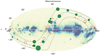 |
Fig. 1. Sky distribution in Galactic coordinates of selected (filled green circles) and rejected (unfilled red circles) pulsars from the lists in Tables 1 and B.1. Larger markers denote a higher (median) precision of the measured DM. The dashed blue line marks the ecliptic, and the dashed gray lines show a region of ±20° from the ecliptic. The background shows the merged all-sky Hα map from Finkbeiner (2003). |
Final source selection, encompassing 14 pulsars.
3. Data analysis
In the following, we detail the analysis methods applied to the data to obtain the DM values, disentangle the IISM-induced effects, and identify the pulsars that show persistent SW signatures. We make use of the pulsar timing technique, which keeps track of every pulsar rotation to model the evolution of the pulse period and phase over the time span of our dataset. This allows us to average each observation in time and improve the signal-to-noise ratio (S/N).
3.1. Calculation of the DM values
For all observations, independent of the observing site, we removed radio-frequency interference, corrected for azimuth and elevation-dependent gain using the LOFAR beam model within the DREAMBEAM package2, and applied band limitations to retain a common frequency range between ∼118 and ∼188 MHz3. These operations were carried out using the PSRCHIVE software suite (Hotan et al. 2004; van Straten et al. 2012) and a modified version4 of the COASTGUARD software suite (Lazarus et al. 2016).
For each pulsar, we then computed a DM value per observation through the pulsar timing technique by proceeding as follows. We first selected the dataset that covered the longest time-baseline. These observations were weighted by the square of their S/N, added together, and then fully averaged in time and partially in frequency (usually down to ten frequency channels to increase the S/N5). Finally, the template was smoothed using the wavelet smoothing scheme first introduced by Demorest et al. (2013). We then collected the observations obtained by all the observing sites for that pulsar and fully averaged them in time and partially in frequency to the same resolution of the template. For each observation, we then generated a set of times-of-arrival (ToAs) associated with the frequency channels with the PSRCHIVE software suite by cross-correlating the observation with the reference template.
A few exceptions to the aforementioned general template-generation scheme were adopted in case the pulsar was too faint, or bright but strongly affected by red noise (due to irregularities in the pulsar rotation or extreme IISM-linked DM variations that caused the template to appear broadened). In the first case, we averaged the longest dataset described earlier over frequency and time to then produce an analytic template, obtained by approximating the data-derived pulse profile with a sum of von Mises functions. In the second case, we used a small subset of phase-aligned observations, which were subsequently averaged and smoothed.
After generating a set of frequency-resolved ToAs per observation, we used the TEMPO2 software suite for pulsar timing (Edwards et al. 2006) and the procedure outlined in Tiburzi et al. (2019) to calculate one DM value per observation6. We then combined the DM time series from all the available observing sites, after subtracting the reference DM value.
3.2. Disentangling the IISM contribution
The obtained DM time series show variations due to both the SW and the IISM. To remove the influence of the IISM, we proceeded as follows for each pulsar.
The DM time series was divided into 460-day-long segments centered on the Solar conjunctions, that is, adding an additional 1.5 months of baseline to a 6-month time window on either side of the Solar conjunction. Hence, the segments overlap for about 100 days. Segments that either contained gaps of more than 55 days between successive observations or those where the effective time span is < 368 days (80% of 460 days) were also discarded as they do not provide a long enough baseline to properly define the IISM effects (this only affects initial and final segments).
The DM time series in each segment was modeled in a Bayesian framework as the sum of a spherically symmetric SW model (Eq. (4)), with AAU being a free parameter, and a polynomial to account for the IISM contribution. By simulating DM time series affected by Kolmogorov turbulence (Armstrong et al. 1995), we found that a cubic polynomial was sufficient to model the DM variations due to the IISM on 460-day-long segments (see the validation of the method in Appendix A). To account for any common systematic error in the estimation of the DM uncertainties, we inserted an additional parameter into the model, summed in quadrature with the DM uncertainties in the likelihood function. We used a Markov chain Monte Carlo method (MCMC; implemented using the emcee package; Foreman-Mackey et al. 2013) to obtain the parameters of the cubic polynomial, the uncertainties correction parameter, and the SW amplitude AAU, and to account for the covariance of the SW amplitude with the parameters of the IISM model. We assigned flat priors to the polynomial coefficients as well as a flat and positive prior to the amplitude of the SW model and the uncertainties correction parameter.
As a final step, the modeled IISM contribution was subtracted from the DM time series. In the overlapping region between two successive years, data points that lay within 6 months of the preceding Solar approach were approximated by the plasma model computed for the first year, while data points within 6 months of the following Solar approach were approximated by the one computed for the second year7. After estimating the model, data points collected earlier than 6 months before the first Solar conjunction or later than 6 months after the last Solar conjunction were discarded. As an example of the final result, Fig. 2 shows the IISM disentanglement for PSR J0030+0451.
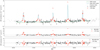 |
Fig. 2. IISM-SW disentanglement in PSR J0030+0451. The upper panel shows the time series of the DM variations and the IISM models (dot-dashed green line) and of the SW and IISM combined (solid blue line). The data used are represented as black dots and red diamonds (where the red diamonds indicate the observations within 50° in Solar elongation and the black dots indicate the observations beyond 50°), while the discarded data points are in gray. Middle panel: DM residuals after subtraction of the IISM model only, and the lowest panel shows the DM residuals after subtraction of both the IISM and the SW models. |
We note here that in Tiburzi et al. (2019) we demonstrated that the spherical model is a poor description of the SW when tested against sufficiently sensitive data. Nevertheless, we have adopted it in the procedure described above for two reasons. First, it was proven to be the better of the two available models compared in that work. Secondly, in Tiburzi et al. (2019) we found that, while the spherical approximation could not model the short-term SW-induced DM variations, it provided a reasonable description of the long-term ones.
3.3. Final selection
The procedure outlined above allowed us to refine our pulsar selection by rejecting those sources where the SW signature is not reliably detected. Specifically, we retained a pulsar if and only if in more than half of the dataset: (a) the model described in the previous section was preferred over an IISM-only model as evaluated by the Bayesian information criterion (BIC), and (b) the posterior distribution of the SW model’s amplitude was significantly different from zero8.
A total of 14 pulsars satisfied these requirements, as reported in Table 1 and Fig. 3 (for the discarded sources, see Table B.1). Among these, there are the PTA class millisecond pulsars J0030+0451, J0034−0534, J1022+1001, J2145−0750, and J2317+1439 (Perera et al. 2019), which, as expected, display the best DM precision of the sample. We consider the 14 selected sources as well suited for studying the electron density in the SW at low frequencies in the Northern Hemisphere. Figure 4 shows that, for equal ecliptic latitudes, the pulsars included in the final selection always present the best DM precision among the sources at the same ecliptic latitudes. The limited cases of sources with high DM precision where the SW is not detected can typically be explained by a combination of low S/N and a poor sampling cadence (e.g., PSR J1024−0719). For the few pulsars in which these causes are not applicable (e.g., PSR J0837+0610), we speculate that the reason lies in an asymmetry of the SW contribution with respect to the heliographic latitude. A more rigorous test of this hypothesis will be presented in a future work through comparisons with data-derived magneto-hydrodynamic simulations of the SW electron density fluctuations, such as EUHFORIA (Poedts & Pomoell 2017).
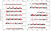 |
Fig. 3. DM time series of the selected pulsars after subtraction of the IISM component. Observations highlighted in red were taken when the Solar elongation of the source was < 50°, and the gray vertical lines mark the modified Julian dates (MJDs) of the Solar conjunctions. For the sake of visual clarity, these plots show only 95% of the most precise measurements, although all data points are used in the analysis. |
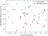 |
Fig. 4. Pulsars included in the final selection (red circles) versus the excluded pulsars (black stars) as a function of ecliptic latitude and the logarithm of the median DM error. |
4. Results
4.1. Performance with respect to a SW model with constant amplitude
Regarding pulsar timing experiments, it is important to understand whether a spherical model of the SW performs better (i.e., yields smaller residuals when subtracted from the observations) when a time-variable or a static amplitude is assumed. With this aim, we repeated the analysis described in Sect. 3.2 on the final pulsar selection by fixing the amplitude for the spherical SW model to a value of 7.9 cm−3 (Madison et al. 2019), and we compared the results. We stress that, for this analysis, we excluded those segments in the pulsar’s datasets where the posterior distribution of the SW amplitude was found to be consistent with zero in the previous section. In Fig. 5, assuming an absence of DM frequency dependence (cf. Cordes et al. 2016), we show the comparison between the two spherical models – with a time-dependent and a time-invariable amplitude – reported through Eq. (1) in terms of residual time delays at 1400 MHz (the main reference frequency for high-precision pulsar timing studies). In particular, we display the rms of the time delays induced by the residual DM fluctuations in the two different analyses, binned in Solar elongation. In Fig. 5, the black dots and red stars refer respectively to a constant- and a variable-amplitude SW model.
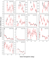 |
Fig. 5. Root-mean-square of the residual timing delays in our data, rescaled to an observing frequency of 1400 MHz. The timing residuals were binned in Solar elongation with a resolution of 5° and an SW model with a time-constant (black) or a variable (red) amplitude was subtracted. The pulsars are sorted by ecliptic latitude. |
By assuming the rms of the residual time delays as a criterion, a model with a variable amplitude performs better than one with a constant amplitude in more than 60% of the cases for Solar elongations up to 20°. The PTA class pulsars of the sample show the most significant improvements depending on the Solar elongation. For example, the rms of the residual time delays decreases by a few tens of sigma9 in PSR J0034−0534 below 15° in Solar elongation, and from ∼15 to ∼10 sigma in PSRs J2145−0750, J1022+1001, and J0030+0451 at the closest Solar elongations.
Nevertheless, Fig. 5 also clearly shows that a simple spherical model, even when a variable amplitude is applied, does not provide a sufficiently precise description of the SW contribution to the DM. This is evident from the level of the residual time delay’s rms at the smallest elongations (< 10° to 20°), which, in the case of the PTA class pulsars (yielding the best DM precision), never reaches the noise floor set by the points at the largest Solar elongations. At the smallest elongations, SW acceleration leads to a steeper decrease in density than implied by a simple inverse square. This is illustrated by Bird et al. (1994), who found that a density model of r−2.54 fit the data inside of 10° elongation better. The bimodal model proposed by You et al. (2007b) used separate density models to account for the fast and slow streams, based on results published by Guhathakurta & Fisher (1995, 1998), Muhleman & Anderson (1981), and Allen (1947), respectively. The results presented here further demonstrate the necessity to account for SW acceleration in measurements taken close to the Sun. This confirms the findings of Tiburzi et al. (2019) and extends them to a larger number of pulsars at different ecliptic latitudes.
4.2. Temporal and latitudinal evolution of the SW density
Our results show that the amplitude of the spherical SW model is not constant with time and ecliptic latitude. This is displayed in the left panel of Fig. 6, which reports the temporal evolution of the aforementioned amplitudes, each obtained from the data of a specific Solar approach for each pulsar. By averaging the computed SW amplitudes (excluding the upper limits) obtained from different pulsars in a given year and latitude range (right panel of Fig. 6), a decreasing trend in time becomes evident at ecliptic latitudes between 5° and 20° as well as between −5° and −10°. The identified decreasing trend may be related to the cyclical Solar activity, which peaked in 2014 and is expected to have reached a minimum in 2020. Conversely, the amplitude of the model does not show an evident decrease in time for pulsars with an ecliptic latitude included between −5° and +5°. This may be due to the shorter distance to the ecliptic with respect to other pulsars, but additional studies are needed to identify the cause of these temporal trends10.
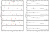 |
Fig. 6. Temporal trend of the amplitude for the SW spherical model, divided into bins of ecliptic latitude, for the individual pulsars (left panel) and averaged year by year (right panel). The gray line marks an amplitude of 7.9 cm−3 (the best-fit value from Madison et al. 2019). All data points are shown with vertical error bars. The upper limits are displayed at the levels of the 95th percentile of the posterior distribution in the left panel and are not considered in the right panel. |
5. Future prospects for the study of SW-induced DM signatures
Here we comment on possible future studies of this kind. Specifically, we identify two possible sources for future studies with LOFAR and comment on the potential for future radio observatories.
5.1. Prospects for LOFAR studies
Some of the pulsar campaigns whose data we have used in this article are carried out with the LOFAR Core at a monthly cadence. As stated in Sect. 2, if a pulsar is observed at a monthly cadence only (i.e., without any coverage from the international stations, which usually observe at a weekly cadence), it has not been taken into consideration for this project. However, it is worth mentioning two particularly promising pulsars for possible SW studies because of their low ecliptic latitude and good DM precision: PSRs J1730−2304 (with a median DM precision of 3 × 10⁻⁴ pc cm−3 and an ecliptic latitude of 0.19°) and J2256−1024 (with a median DM precision of 6 × 10⁻⁵ pc cm−3 and an ecliptic latitude of −3.41°). New observing campaigns with the LOFAR Core have recently been carried out with the aims of (a) increasing the observing coverage of these and other pulsars during their Solar approaches and (b) collecting simultaneous data for interplanetary scintillation studies to be compared with the pulsar-based results and white-light observations, as detailed below. Moreover, as the decreasing trend shown in many pulsars might be related to the Solar cycle, future LOFAR observations may be able to detect an increase in the excess DM induced by the SW as the Solar activity is expected to increase in the coming years.
Further research is also planned to investigate more robust methods to estimate the SW contribution to the pulsar DM. This includes more detailed investigations of the bimodal approach of You et al. (2007b), incorporating a direct comparison of the LoS with Carrington maps of coronal white light to ascertain regions of fast and slow SWs, as in the approach taken recently by Tokumaru et al. (2020). Other approaches under investigation involve the use of 3D tomographic reconstructions of velocity and density in the inner heliosphere, obtained from observations of interplanetary scintillation and coronal white light (e.g., Jackson et al. 2020, and references therein), and the use of space weather models such as EUHFORIA (Poedts & Pomoell 2017).
5.2. SW studies with next-generation telescopes
While we have demonstrated the capabilities of LOFAR in monitoring the SW with pulsars, its activity could be complemented by the utilization of other telescopes. Observing facilities in the Southern Hemisphere with the capability of covering low-frequency ranges, such as Murchinson Widefield Array (Tingay et al. 2013) and the upcoming SKA1-Low (Braun et al. 2015), will have access to a different and more extended set of pulsars in comparison to LOFAR because of a more prolonged visibility of the inner Galaxy. Furthermore, with telescopes such as CHIME (Bandura et al. 2014), MeerKAT (Jonas 2009), SKA1-Low, LOFAR2.0 (the upcoming upgrade of LOFAR), and NenuFAR11 (Bondonneau et al. 2020), there will be access to a wider frequency bandwidth, with a consequential enabling of an increased range of scientific studies. As some of these facilities have the possibility of multi-beaming and sub-arraying, they will also be able to track more pulsars simultaneously, hence reducing the times of the observing campaigns.
6. Conclusions
We have presented a study of the impact of the SW on a large sample of pulsars observed for up to 6 years with the LOFAR telescope. This study has demonstrated that the spherically symmetric and static SW model, which is commonly used in pulsar timing experiments, can be improved by allowing a time-variable amplitude, but that these improvements do not suffice for correcting the SW impact at the levels required for high-precision pulsar timing experiments (consistent with our earlier findings in Tiburzi et al. 2019). For PTA class pulsars in particular, the residuals between observations taken at small Solar elongations (< 10° to 20°) and the corresponding model are not able to reach the noise floor set by residuals corresponding to larger Solar elongations. As Tiburzi et al. (2016) demonstrated that the SW is a potential source of false gravitational wave detections, it is then advisable to adopt time-variable SW amplitudes and carefully treat observations taken during Solar conjunction within high-precision pulsar timing experiments.
Moreover, the data indicated that the amplitude of the spherical model has a dependence on time for pulsars whose ecliptic latitudes lie either between −10° and −5° or +5° and +20°. In particular, the amplitude decreases from the first half of the observed time span to the second half of that time span. On the other hand, the amplitude tends to remain constant for pulsars with an ecliptic latitude included between −5° and +5°. Additional studies will be necessary to recognize the cause of these trends and determine whether they are in connection to the Solar cycle activity.
While the investigation of new SW models for high-precision pulsar timing was not within the scope of the current work, a series of measures can be adopted to mitigate the SW-induced noise:
-
Carrying out observations with wideband observing receivers, in combination with the usage of frequency-resolved templates, may allow a precise determination of time-dependent DMs (due to the IISM, the SW, or both) that can be then used to correct the noise induced by variable dispersion.
-
Carrying out simultaneous observations at low and high frequency. A precise DM determination can be obtained thanks to the low-frequency data, that can then be used to correct the high-frequency ToAs.
-
If obtaining simultaneous observations is not possible, carrying out high-cadence, low-frequency observations (ideally once every two or three days) for two weeks around the Solar conjunction may be helpful. The DM values obtained from these observations can be interpolated and used as a correction scheme for high-frequency observations. The high cadence of the observations is important in this case because, as shown by Niu et al. (2017), the fast SW variability may invalidate the DM corrections if the high- and low-frequency observations are separated by more than one day.
-
For pulsars with a flat spectral index, it may be meaningful to carry out observations at very high frequencies (at S band or more), where the DM-induced noise is marginal, and apply the spherical SW model by choosing an amplitude according to, for example, the results of this article depending on the pulsar’s ecliptic latitude. However, this approachimplies that a certain amount of timing noise will be left in the data, especially the data taken close to the Solar conjunction. Moreover, Lam et al. (2018) demonstrated that observing frequencies < 1 GHz are more optimal for achieving high precision in pulsar timing experiments.
While assuming the absence of frequency-dependent DM or time-variable scattering, these actions will be useful to diminish the impact of the SW in pulsar timing experiments. However, the development of a new, performing model is desirable for the future steps of PTA experiments.
7. Data availability
The data underlying this article that were collected with the International LOFAR Stations and with the LOFAR Core under still-private observing programs will be shared on reasonable request to the corresponding author. The data underlying this article collected with the LOFAR Core and under public observing programs are available online12.
The initial timing models, the ToA files, and the DM time series for the pulsars used in this article have been publicly available on Zenodo since January 1, 202113.
Part of the reported values come from the ATNF pulsar catalog, https://www.atnf.csiro.au/research/pulsar/psrcat/ (Manchester et al. 2005).
Band-limiting is necessary to avoid biases in our results because the observing sites record slightly different original bandwidths. The indicated frequency range is common to all of the observing sites (for more details, see Donner et al. 2019; Tiburzi et al. 2019).
https://github.com/larskuenkel/iterative_cleaner (see also Kuenkel 2017).
For particularly faint pulsars, we applied a larger frequency-averaging factor.
We note that, as for Tiburzi et al. (2019), the DM time derivatives included in the original timing model for that pulsar were only applied to properly de-disperse the template and frequency-average the observations, and they were not used in the subsequent determination of the DM variations.
The overlap between adjacent years guarantees a continuous and smooth IISM model across multiple years.
In PSR J1300+1240, only the first two years (out of a total of five) meet the requirements. However, we included it in the final selection after visually inspecting the DM time series and manually examining the results.
Measured as (rmsC, i − rmsV, i)/ermsV, i, with rmsV, i and rmsC, i being the rms of the residuals left by, respectively, the spherical model with a time-dependent amplitude and the spherical model with a time-invariable amplitude at Solar elongation i, and ermsV, i being the uncertainty to rmsV, i.
Because the spherical model is known to be an imperfect SW approximation (Tiburzi et al. 2019), we report an analogous overview of the DM variations in Appendix C.
Acknowledgments
This work is part of the research program Soltrack with project number 016.Veni.192.086, which is partly financed by the Dutch Research Council (NWO). The authors thank the anonymous referee for their support and useful comments. This paper is partially based on data obtained with: (i) the German stations of the International LOFAR Telescope (ILT), constructed by ASTRON (van Haarlem et al. 2013) and operated by the German LOng Wavelength (GLOW) consortium (https://www.glowconsortium.de/) during station-owners time and proposals LC0_014, LC1_048, LC2_011, LC3_029, LC4_025, LT5_001, LC9_039, LT10_014; (ii) the LOFAR core, during proposals LC0_011, DDT0003, LC1_027, LC1_042, LC2_010, LT3_001, LC4_004, LT5_003, LC9_041, LT10_004, LPR12_010; (iii) the Swedish station of the ILT during observing proposals carried out from May 2015 to January 2018. We made use of data from the Effelsberg (DE601) LOFAR station funded by the Max-Planck-Gesellschaft; the Unterweilenbach (DE602) LOFAR station funded by the Max-Planck-Institut für Astrophysik, Garching; the Tautenburg (DE603) LOFAR station funded by the State of Thuringia, supported by the European Union (EFRE) and the Federal Ministry of Education and Research (BMBF) Verbundforschung project D-LOFAR I (grant 05A08ST1); the Potsdam (DE604) LOFAR station funded by the Leibniz-Institut für Astrophysik, Potsdam; the Jülich (DE605) LOFAR station supported by the BMBF Verbundforschung project D-LOFAR I (grant 05A08LJ1); and the Norderstedt (DE609) LOFAR station funded by the BMBF Verbundforschung project D-LOFAR II (grant 05A11LJ1). The observations of the German LOFAR stations were carried out in the stand-alone GLOW mode, which is technically operated and supported by the Max-Planck-Institut für Radioastronomie, the Forschungszentrum Jülich and Bielefeld University. We acknowledge support and operation of the GLOW network, computing and storage facilities by the FZ-Jülich, the MPIfR and Bielefeld University and financial support from BMBF D-LOFAR III (grant 05A14PBA) and D-LOFAR IV (grants 05A17PBA and 05A17PC1), and by the states of Nordrhein-Westfalia and Hamburg. MB acknowledges support from the Deutsche Forschungsgemeinschaft under Germany’s Excellence Strategy – EXC 2121 “Quantum Universe” – 390833306. CT acknowledges support from Onsala Space Observatory for the provisioning of its facilities/observational support. The Onsala Space Observatory national research infrastructure is funded through Swedish Research Council grant No 2017-00648. GS was supported by the Netherlands Organization for Scientific Research NWO (TOP2.614.001.602). JPWV acknowledges support by the Deutsche Forschungsgemeinschaft (DFG) through the Heisenberg program (Project No. 433075039).
References
- Allen, C. W. 1947, MNRAS, 107, 426 [NASA ADS] [Google Scholar]
- Archibald, A. M., Gusinskaia, N. V., Hessels, J. W. T., et al. 2018, Nature, 559, 73 [Google Scholar]
- Armstrong, J. W., Rickett, B. J., & Spangler, S. R. 1995, ApJ, 443, 209 [Google Scholar]
- Bandura, K., Addison, G. E., Amiri, M., et al. 2014, in Ground-based and Airborne Telescopes V, eds. L. M. Stepp, R. Gilmozzi, & H. J. Hall, SPIE Conf. Ser., 9145, 914522 [Google Scholar]
- Bird, M. K., Volland, H., Paetzold, M., et al. 1994, ApJ, 426, 373 [Google Scholar]
- Bondonneau, L., Grießmeier, J. M., Theureau, G., et al. 2020, A&A, submitted [arXiv:2009.02076] [Google Scholar]
- Braun, R., Bourke, T., Green, J. A., Keane, E., & Wagg, J. 2015, Advancing Astrophysics with the Square Kilometre Array (AASKA14), 174 [Google Scholar]
- Burke-Spolaor, S., Taylor, S. R., Charisi, M., et al. 2019, A&ARv, 27, 5 [Google Scholar]
- Caballero, R. N., Guo, Y. J., Lee, K. J., et al. 2018, MNRAS, 481, 5501 [Google Scholar]
- Coles, W. A. 1996, Ap&SS, 243, 87 [Google Scholar]
- Cordes, J. M., Shannon, R. M., & Stinebring, D. R. 2016, ApJ, 817, 16 [Google Scholar]
- Demorest, P. B., Ferdman, R. D., Gonzalez, M. E., et al. 2013, ApJ, 762, 94 [Google Scholar]
- Donner, J. Y., Verbiest, J. P. W., Tiburzi, C., et al. 2019, A&A, 624, A22 [NASA ADS] [CrossRef] [EDP Sciences] [Google Scholar]
- Donner, J. Y., Verbiest, J. P. W., Tiburzi, C., et al. 2020, A&A, 644, A153 [EDP Sciences] [Google Scholar]
- Edwards, R. T., Hobbs, G. B., & Manchester, R. N. 2006, MNRAS, 372, 1549 [Google Scholar]
- Finkbeiner, D. P. 2003, ApJS, 146, 407 [Google Scholar]
- Foreman-Mackey, D., Hogg, D. W., Lang, D., & Goodman, J. 2013, PASP, 125, 306 [Google Scholar]
- Guhathakurta, M., & Fisher, R. R. 1995, Geophys. Res. Lett., 22, 1841 [Google Scholar]
- Guhathakurta, M., & Fisher, R. 1998, ApJ, 499, L215 [Google Scholar]
- Hobbs, G., Guo, L., Caballero, R. N., et al. 2020, MNRAS, 491, 5951 [Google Scholar]
- Hotan, A. W., van Straten, W., & Manchester, R. N. 2004, PASA, 21, 302 [Google Scholar]
- Jackson, B. V., Buffington, A., Cota, L., et al. 2020, Front. Astron. Space Sci., 7, 76 [Google Scholar]
- Janssen, G., Hobbs, G., McLaughlin, M., et al. 2015, Advancing Astrophysics with the Square Kilometre Array (AASKA14), 37 [Google Scholar]
- Jonas, J. L. 2009, IEEE Proc., 97, 1522 [Google Scholar]
- Kuenkel, L. 2017, LOFAR Studies of Interstellar Scintillation [Google Scholar]
- Lam, M. T., Cordes, J. M., Chatterjee, S., et al. 2016, ApJ, 819, 155 [Google Scholar]
- Lam, M. T., McLaughlin, M. A., Cordes, J. M., Chatterjee, S., & Lazio, T. J. W. 2018, ApJ, 861, 12 [Google Scholar]
- Lazarus, P., Karuppusamy, R., Graikou, E., et al. 2016, MNRAS, 458, 868 [Google Scholar]
- Lentati, L., Shannon, R. M., Coles, W. A., et al. 2016, MNRAS, 458, 2161 [Google Scholar]
- Lorimer, D. R., & Kramer, M. 2004, Handbook of Pulsar Astronomy (Cambridge: Cambridge University Press) [Google Scholar]
- Madison, D. R., Cordes, J. M., Arzoumanian, Z., et al. 2019, ApJ, 872, 150 [Google Scholar]
- Manchester, R. N., & Taylor, J. H. 1972, Astrophys. Lett., 10, 67 [NASA ADS] [Google Scholar]
- Manchester, R. N., Hobbs, G. B., Teoh, A., & Hobbs, M. 2005, AJ, 129, 1993 [NASA ADS] [CrossRef] [Google Scholar]
- Muhleman, D. O., & Anderson, J. D. 1981, ApJ, 247, 1093 [Google Scholar]
- Niu, Z.-X., Hobbs, G., Wang, J.-B., & Dai, S. 2017, Res. Astron. Astrophys., 17, 103 [Google Scholar]
- Perera, B. B. P., DeCesar, M. E., Demorest, P. B., et al. 2019, MNRAS, 490, 4666 [Google Scholar]
- Poedts, S., & Pomoell, J. 2017, EGU General Assembly Conference Abstracts, 7396 [Google Scholar]
- Porayko, N. K., Noutsos, A., Tiburzi, C., et al. 2019, MNRAS, 483, 4100 [Google Scholar]
- Schwenn, R. 1990, in Large-Scale Structure of the Interplanetary Medium, eds. R. Schwenn, & E. Marsch, 99 [Google Scholar]
- Schwenn, R. 2006, Liv. Rev. Sol. Phys., 3, 2 [Google Scholar]
- Shao, L., Caballero, R. N., Kramer, M., et al. 2013, Class. Quant. Grav., 30, 165019 [Google Scholar]
- Siemens, X., Ellis, J., Jenet, F., & Romano, J. D. 2013, Class. Quant. Grav., 30, 224015 [Google Scholar]
- Stappers, B. W., Hessels, J. W. T., Alexov, A., et al. 2011, A&A, 530, A80 [NASA ADS] [CrossRef] [EDP Sciences] [Google Scholar]
- Tiburzi, C. 2018, PASA, 35, e013 [Google Scholar]
- Tiburzi, C., Hobbs, G., Kerr, M., et al. 2016, MNRAS, 455, 4339 [Google Scholar]
- Tiburzi, C., Verbiest, J. P. W., Shaifullah, G. M., et al. 2019, MNRAS, 487, 394 [Google Scholar]
- Tingay, S. J., Goeke, R., Bowman, J. D., et al. 2013, PASA, 30, e007 [Google Scholar]
- Tokumaru, M., Tawara, K., Takefuji, K., Sekido, M., & Terasawa, T. 2020, Sol. Phys., 295, 80 [Google Scholar]
- Vallisneri, M., Taylor, S. R., Simon, J., et al. 2020, ApJ, 893, 112 [Google Scholar]
- van Haarlem, M. P., Wise, M. W., Gunst, A. W., et al. 2013, A&A, 556, A2 [NASA ADS] [CrossRef] [EDP Sciences] [Google Scholar]
- van Straten, W., & Bailes, M. 2011, PASA, 28, 1 [Google Scholar]
- van Straten, W., Demorest, P., & Osłowski, S. 2012, Astron. Res. Technol., 9, 237 [Google Scholar]
- Verbiest, J. P. W., Lentati, L., Hobbs, G., et al. 2016, MNRAS, 458, 1267 [Google Scholar]
- Voisin, G., Cognard, I., Freire, P. C. C., et al. 2020, A&A, 638, A24 [CrossRef] [EDP Sciences] [Google Scholar]
- You, X. P., Hobbs, G. B., Coles, W. A., Manchester, R. N., & Han, J. L. 2007a, ApJ, 671, 907 [Google Scholar]
- You, X. P., Hobbs, G., Coles, W. A., et al. 2007b, MNRAS, 378, 493 [Google Scholar]
- You, X. P., Coles, W. A., Hobbs, G. B., & Manchester, R. N. 2012, MNRAS, 422, 1160 [Google Scholar]
Appendix A: Effectiveness of the IISM-SW disentangling scheme
To confirm that our choice of a third-order polynomial is a sufficient description of the IISM contributions, we simulated 500 DM time series affected by Kolmogorov turbulence and white noise as drawn from a zero-mean Gaussian population with a variance of 1 × 10⁻⁴ pc cm−3, and we have attributed irregular error bars to match the ones of PSR J1022+1001. To this time series, we then added the SW contribution from a spherically symmetric model, with a variable amplitude per year. This final dataset was then analyzed following the steps detailed in Sect. 3.2. For each year and injected value of the spherical SW amplitude, as shown in Fig. A.1, we were able to recover a statistically comparable value of the amplitude of the spherical SW model.
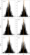 |
Fig. A.1. Injected (dashed orange lines) and recovered (filled black histograms) values of the amplitude of the spherically symmetric SW model. |
We further tested whether the third-order polynomial model is able to account for the IISM contribution only. To this end, we repeated the above simulations without adding the SW contribution, and we analyzed the DM time series using the MCMC algorithm described in Sect. 3.2, modified to apply a segment-by-segment cubic-only model. To determine the success rate of the modeling procedure, we used a two-tailed Kolmogorov–Smirnov (KS) test. The results report that, in 100% of the cases, the distribution of the residuals after applying the cubic model are identical to a zero-mean Gaussian distribution. This confirms the ability of our algorithm in removing the IISM contribution from the DM time series.
To test whether our algorithm performs as well on real, irregular DM time series as it does on simulated data, we repeated the analysis we just described on the DM time series of the four millisecond pulsars presented in Donner et al. (2020), namely PSRs J0218+4232, J0740+6620, J1125+7819, and J1640+2224. These sources have a high ecliptic latitude (> 30°); therefore, we can assume that they are only affected by IISM-induced variations. We used the IISM-only MCMC algorithm that we described in the previous paragraph (i.e., modified to apply a segment-by-segment cubic-only model) to model the IISM variations presented by these pulsars. The two-tailed KS test showed that, after modeling the DM time series with the results of our algorithm, the resulting residuals were just as compatible with a zero-mean Gaussian distribution (see Fig. A.2). Thus we are able to demonstrate that our modeling method leads to the IISM contribution being successfully disentangled from the SW component.
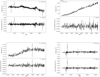 |
Fig. A.2. DM time series of the four tested millisecond pulsars (upper panel of each quadrant) and their post-modeling residuals (bottom panels). |
Appendix B: Pulsars without significant SW signatures
Table B.1 reports the investigated pulsars that do not show significant SW signatures.
Investigated pulsars that do not show significant SW signatures.
Appendix C: Variations in the SW impact on the DM time series
Section 4.2 reports the amplitude of the spherical SW model as variables across the years for a number of pulsars. However, Tiburzi et al. (2019; and this article) showed the spherical model to be an imperfect SW approximation. As an additional confirmation of the detected variability of the SW contribution, we also examined the DM variations themselves, after subtracting the IISM component. Figure C.1 shows the averages of DM variations as a function of the Solar elongation (in 5° bins, up to 50°) from all 14 pulsars, organized by ecliptic latitude and time of observation. As for the amplitudes of the spherical SW model, it is possible to verify that the magnitude of the DM variations also decreases in time within the ecliptic latitude ranges spanning from 20° to 5° and from −5° to −10°. For example, for pulsars with ecliptic latitudes ranging from 15° to 20°, the average DM variations at Solar elongations smaller than 20° decrease from 4.2 × 10⁻⁴ pc cm3 to 5 × 10⁻⁵ pc cm3. Similarly, pulsars whose ecliptic latitudes range between 5° and 10° have DM variations at Solar elongations < 10°, which drop from 1.2 × 10⁻³ pc cm3 to 5.2 × 10⁻⁴ pc cm3 across the time span. On the other hand, the DM variations for pulsars with ecliptic latitudes included between −5° and 5° tend to fluctuate without showing a clear decreasing trend. This confirms the trend seen in Fig. 6.
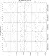 |
Fig. C.1. Average DM variations (after the subtraction of the IISM) as a function of Solar elongation, divided per time and ecliptic latitude. All data points are shown with vertical error bars. |
All Tables
All Figures
|
Fig. 1. Sky distribution in Galactic coordinates of selected (filled green circles) and rejected (unfilled red circles) pulsars from the lists in Tables 1 and B.1. Larger markers denote a higher (median) precision of the measured DM. The dashed blue line marks the ecliptic, and the dashed gray lines show a region of ±20° from the ecliptic. The background shows the merged all-sky Hα map from Finkbeiner (2003). |
| In the text | |
|
Fig. 2. IISM-SW disentanglement in PSR J0030+0451. The upper panel shows the time series of the DM variations and the IISM models (dot-dashed green line) and of the SW and IISM combined (solid blue line). The data used are represented as black dots and red diamonds (where the red diamonds indicate the observations within 50° in Solar elongation and the black dots indicate the observations beyond 50°), while the discarded data points are in gray. Middle panel: DM residuals after subtraction of the IISM model only, and the lowest panel shows the DM residuals after subtraction of both the IISM and the SW models. |
| In the text | |
|
Fig. 3. DM time series of the selected pulsars after subtraction of the IISM component. Observations highlighted in red were taken when the Solar elongation of the source was < 50°, and the gray vertical lines mark the modified Julian dates (MJDs) of the Solar conjunctions. For the sake of visual clarity, these plots show only 95% of the most precise measurements, although all data points are used in the analysis. |
| In the text | |
|
Fig. 4. Pulsars included in the final selection (red circles) versus the excluded pulsars (black stars) as a function of ecliptic latitude and the logarithm of the median DM error. |
| In the text | |
|
Fig. 5. Root-mean-square of the residual timing delays in our data, rescaled to an observing frequency of 1400 MHz. The timing residuals were binned in Solar elongation with a resolution of 5° and an SW model with a time-constant (black) or a variable (red) amplitude was subtracted. The pulsars are sorted by ecliptic latitude. |
| In the text | |
|
Fig. 6. Temporal trend of the amplitude for the SW spherical model, divided into bins of ecliptic latitude, for the individual pulsars (left panel) and averaged year by year (right panel). The gray line marks an amplitude of 7.9 cm−3 (the best-fit value from Madison et al. 2019). All data points are shown with vertical error bars. The upper limits are displayed at the levels of the 95th percentile of the posterior distribution in the left panel and are not considered in the right panel. |
| In the text | |
|
Fig. A.1. Injected (dashed orange lines) and recovered (filled black histograms) values of the amplitude of the spherically symmetric SW model. |
| In the text | |
|
Fig. A.2. DM time series of the four tested millisecond pulsars (upper panel of each quadrant) and their post-modeling residuals (bottom panels). |
| In the text | |
|
Fig. C.1. Average DM variations (after the subtraction of the IISM) as a function of Solar elongation, divided per time and ecliptic latitude. All data points are shown with vertical error bars. |
| In the text | |
Current usage metrics show cumulative count of Article Views (full-text article views including HTML views, PDF and ePub downloads, according to the available data) and Abstracts Views on Vision4Press platform.
Data correspond to usage on the plateform after 2015. The current usage metrics is available 48-96 hours after online publication and is updated daily on week days.
Initial download of the metrics may take a while.