| Issue |
A&A
Volume 647, March 2021
|
|
|---|---|---|
| Article Number | A166 | |
| Number of page(s) | 16 | |
| Section | Cosmology (including clusters of galaxies) | |
| DOI | https://doi.org/10.1051/0004-6361/202039786 | |
| Published online | 29 March 2021 | |
The relation between Lyα absorbers and local galaxy filaments
Institut für Physik und Astronomie, Universität Potsdam, Karl-Liebknecht-Str. 24/25, 14476 Golm, Germany
e-mail: This email address is being protected from spambots. You need JavaScript enabled to view it.
Received:
29
October
2020
Accepted:
1
February
2021
Abstract
Context. The intergalactic medium (IGM) is believed to contain the majority of baryons in the universe and to trace the same dark matter structure as galaxies, forming filaments and sheets. Lyα absorbers, which sample the neutral component of the IGM, have been extensively studied at low and high redshift, but the exact relation between Lyα absorption, galaxies, and the large-scale structure is observationally not well constrained.
Aims. In this study, we aim at characterising the relation between Lyα absorbers and nearby over-dense cosmological structures (galaxy filaments) at recession velocities Δv ≤ 6700 km s−1 by using archival observational data from various instruments.
Methods. We analyse 587 intervening Lyα absorbers in the spectra of 302 extragalactic background sources obtained with the Cosmic Origins Spectrograph (COS) installed on the Hubble Space Telescope (HST). We combine the absorption line information with galaxy data of five local galaxy filaments from the V8k catalogue.
Results. Along the 91 sightlines that pass close to a filament, we identify 215 (227) Lyα absorption systems (components). Among these, 74 Lyα systems are aligned in position and velocity with the galaxy filaments, indicating that these absorbers and the galaxies trace the same large-scale structure. The filament-aligned Lyα absorbers have a ∼90% higher rate of incidence (d𝒩/dz = 189 for log N(H I) ≥ 13.2) and a slightly shallower column density distribution function slope (−β = −1.47) relative to the general Lyα population at z = 0, reflecting the filaments’ matter over-density. The strongest Lyα absorbers are preferentially found near galaxies or close to the axis of a filament, although there is substantial scatter in this relation. Our sample of absorbers clusters more strongly around filament axes than a randomly distributed sample would do (as confirmed by a Kolmogorov–Smirnov test), but the clustering signal is less pronounced than for the galaxies in the filaments.
Key words: galaxies: halos / intergalactic medium / quasars: absorption lines / large-scale structure of Universe / techniques: spectroscopic / ultraviolet: general
© ESO 2021
1. Introduction
It is generally accepted that the intergalactic medium (IGM) contains the majority of the baryons in the universe (e.g., Shull 2003; Lehner et al. 2007; Danforth & Shull 2008; Richter et al. 2008; Shull et al. 2012; Danforth et al. 2016), making it a key component in understanding cosmological structure formation. It is estimated that about 30% of the baryons at low-z are in the form of photoionised hydrogen at a temperature of ≲104 K (Penton et al. 2000; Lehner et al. 2007; Danforth & Shull 2008; Shull et al. 2012; Tilton et al. 2012; Danforth et al. 2016), while the collapsed, shock-heated warm-hot intergalactic medium (WHIM) at T ∼ 105 − 106 K contains at least 20% (Richter et al. 2006a,b; Lehner et al. 2007). Cosmological simulations indicate that the WHIM may contribute up to 50% of the baryons in the low-z universe (Cen & Ostriker 1999; Davé et al. 1999; Shull et al. 2012; Martizzi et al. 2019). This makes the IGM an important reservoir of baryons used by galaxies to fuel star formation. Indeed, to explain current rates of star formation, such a baryon reservoir is needed (e.g., Erb 2008; Prochaska & Wolfe 2009; Genzel et al. 2010). In this way, the evolution of galaxies is tied to the properties and the spatial distribution of the IGM.
The relation between the IGM and galaxies is not one-way, however, as galaxies influence their surroundings by ejecting hot gas into their circumgalactic medium (CGM) via active galactic nucleus (AGN) feedback (e.g., Bower et al. 2006; Davies et al. 2019) and, particularly in the early universe, via supernova explosions (Madau et al. 2001; Pallottini et al. 2014). Thus, there is a large-scale exchange of matter and energy between the galaxies and the surrounding IGM, and each environment influences the evolution of the other. One observational method for studying the gas circulation processes between galaxies and the IGM is the analysis of intervening Lyman α (Lyα) absorption in the spectra of distant AGN, which are believed to trace the large-scale gaseous environment of galaxies. Generally, an anti-correlation between Lyα absorber strength and the galaxy impact parameter is found for absorbers that are relatively close to galaxies (e.g., Chen et al. 2001; Bowen et al. 2002; Wakker & Savage 2009; French & Wakker 2017).
The IGM is not only tied to the galaxies; it is also expected to trace the dark matter distribution and can, therefore, provide insights into the large-scale structure of the universe. This large-scale structure has been mapped by galaxy surveys such as the Two-degree Field Galaxy Redshift Survey and the Sloan Digital Sky Survey (SDSS; Colless et al. 2001; York et al. 2000). Studying the IGM absorber distribution at low redshift allows for a comparison with data from these galaxy surveys. Already more than 25 years ago, Morris et al. (1993) studied the spectrum of the bright quasar 3C 273 and mapped Lyα absorbers along this line of sight together with galaxies in its vicinity. They found that Lyα absorbers cluster less strongly around galaxies than the galaxies do among themselves. This can be interpreted as most of the Lyα absorbers being truly intergalactic in nature, following the filamentary large-scale structure rather than the position of individual galaxies.
More recently, Tejos et al. (2016) studied Lyα and O VI absorption in a single sightline in regions between galaxy clusters. The detected over-density of narrow and broad Lyα absorbers hints at the presence of filamentary gas connecting the clusters. A different approach was taken by Wakker et al. (2015). Instead of mapping gas along an isolated sightline, they used several sightlines passing through a known galaxy filament. By comparing the relation of Lyα equivalent width with both galaxy and filament impact parameters, Wakker et al. (2015) conclude that Lyα absorbers are best described in the context of large-scale structure rather than as tracers of individual galaxy halos. While there is a relation between strong (N(H I) > 1015 cm−2) absorbers and the CGM of galaxies, weak Lyα absorbers are more likely to be associated with filaments. This view is also supported by Penton et al. (2002), who find that weak absorbers do not show a correlation between equivalent width and impact parameter to the nearest galaxy, while stronger absorbers do. By comparing the position of their sample of Lyα absorbers relative to galaxies in filaments, they conclude that the absorbers align with the filamentary structure. Evidence for absorbers tracing an extensive, intra-group medium comes from the other recent surveys of Stocke et al. (2013) and Keeney et al. (2018).
While the correlation between the Lyα equivalent width and the galaxy impact parameter seems to indicate that these absorbers are somehow associated with galaxies (e.g., by the gravitational potential), studies such as Wakker et al. (2015) and Tejos et al. (2016) show that at least some of the absorbers are associated with the cosmological large-scale structure. Others studies (Bowen et al. 2002; Wakker & Savage 2009) conclude that their data simply do not yield any definite conclusions on this aspect (see also Penton et al. 2002; Prochaska et al. 2011; Tejos et al. 2014). Therefore, the question of how Lyα absorbers at z = 0 are linked to galaxies and the large-scale cosmological structure remains unresolved. Clearly, additional absorption line studies that improve the currently limited statistics on the absorber-to-galaxy-connection are desired.
In this paper, we systematically investigate the properties of z = 0 Lyα absorbers and their connection to the local galaxy environments and the surrounding large-scale structure. For this, we follow an approach similar to that of Wakker et al. (2015). We combine the information on local galaxy filaments mapped by Courtois et al. (2013) with archival UV absorption line data from the Cosmic Origins Spectrograph (COS) installed on the Hubble Space Telescope (HST).
Information on the galaxy sample used in this study is provided in Sect. 2. In Sect. 3, the HST/COS data are described and information on the absorption line measurements is given. Details on the galaxy filaments are presented in Sect. 4. In Sect. 5, we investigate the relation between absorbers and galaxies, whereas in Sect. 6 we focus on the relation between absorbers and filaments. In Sect. 7, we discuss our findings and compare them with previous studies. Finally, we summarise and conclude our study in Sect. 8.
2. Galaxy data
Courtois et al. (2013) used the V8k catalogue of galaxies to map galaxy filaments in the nearby universe. This catalogue is available from the Extragalactic Distance Database1 (EDD; Tully et al. 2009). It is a compilation of different surveys, including John Huchra’s ‘ZCAT’ and the IRAS Point Source Catalog redshift survey with its extensions to the Galactic plane (Saunders et al. 2000a,b). In total, the catalogue consists of ∼30 000 galaxies, all with velocities less than 8000 km s−1. It is complete up to MB = −16 for galaxies at 1000 km s−1, while at 8000 km s−1, it contains one in 13 of the MB = −16 galaxies. A radial velocity of 8000 km s−1 corresponds to a cosmological distance of d ∼ (114 km s . The distance to the Centaurus Cluster (v ∼ 3000 km s−1) is ∼40 Mpc. As described in Sect. 3, the velocity range studied in this work extends up to v ∼ 6700 km s−1, which corresponds to λ ∼ 1243 Å. We note that distance estimates to galaxies within 3000 km s−1 in the V8k catalogue are adjusted to match the Virgo-flow model by Shaya et al. (1995). The relatively uniform sky coverage – with the exception of the zone of avoidance (ZOA) – of the V8k survey combined with the broad range of galaxy types make it suitable for qualitative work (Courtois et al. 2013).
The distribution of apparent and absolute B-band magnitudes as well as log(L/L*) for all galaxies of the V8k catalogue is presented in Fig. 1. As can be seen from this distribution, the V8k catalogue is largely insensitive to dwarf galaxies with luminosities log(L/L*) ≤ − 0.5. This needs to be kept in mind for our later discussion of the absorber-galaxy relation in Sects. 5 and 6. We decided to not add supplementary galaxy data from other surveys because the sky coverage of such a mixed galaxy sample would be quite inhomogeneous, which would introduce an additional bias to the absorber-galaxy statistics.
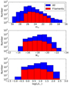 |
Fig. 1. Histogram of apparent and absolute B-band magnitudes and luminosities for all galaxies of the V8k catalogue. |
In the upper panel of Fig. 2, we show the sky distribution of the galaxies in the various filaments, as defined in Courtois et al. (2013). The galaxies in these filaments have radial velocities in the range v = 750 − 5900 km s−1. All filaments feed into the Centaurus Cluster located at l ∼ 300° and b ∼ 20°. The large concentration of galaxies in the green filament, between l ∼ 260 − 300° and b ∼ 60 − 70°, is due to the Virgo Cluster.
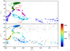 |
Fig. 2. All-sky map of filaments in the local Universe. Upper panel: sky distribution of galaxies from V8k belonging to filaments as defined in Courtois et al. (2013). The different colours indicate different galaxy filaments. Several important clusters are noted. Lower panel: sky distribution of HST/COS sightlines passing close to a filament (black circles) and HST/COS sightlines not belonging to a filament (grey circles) plotted together with the galaxies from the V8k catalogue belonging to filaments (colour-coded according to velocity). |
3. Absorption line data
3.1. HST/COS observations
In this study, we made use of ancillary HST/COS data, as retrieved from the HST Science Archive at the Canadian Astronomy Data Centre (CADC). The total sample consists of 302 quasar (QSO2) sightlines, all of which were reduced following the procedures described in Richter et al. (2017).
Since the Lyα absorption (λ0 = 1215.67 Å) in the spectra studied here falls within the wavelength range between 1215 and 1243 Å, we made use of the data from the COS G130M grating. This grating covers a wavelength range from 1150−1450 Å and has a resolving power of R = 16 000 − 21 000 (Green et al. 2012; Dashtamirova & Fischer 2018). The data quality in our COS sample is quite diverse, with signal-to-noise ratios (S/N) per resolution element varying substantially (between 3 and 130; see Fig. A.1).
We also checked for metal absorption in the Lyα absorbers, considering the transitions of Si IIIλ1206.50, the Si II doublet λ1190.42; 1193.29, Si IIλ1260.42, Si IIλ1526.71, the Si IV doublet λ1393.76; 1402.77, C IIλ1334.53, and the C IV doublet λ1548.20; 1550.77. For the lines at λ > 1450 Å, data from the COS G160M grating were used, which covers λ = 1405−1775 Å.
The QSO sightlines are plotted on top of the V8k galaxy filaments in the lower panel of Fig. 2. The sky coverage of the sightlines is noticeably better in the upper hemisphere. As can be seen, the majority of the sightlines do not pass through the centres of the filaments, but rather are located at the filament edges.
A reason for sightlines not going directly through filaments could be extinction. This especially holds true for dense regions such as the Virgo Cluster, where the extinction is high. On the other hand, the Virgo Cluster is a nearby cluster and might be better studied than random regions on the sky. From the COS sightlines shown in the lower panel of Fig. 2, no clear bias can be seen, except for the northern versus southern hemisphere.
3.2. Absorber sample and spectral analysis
For all 302 COS spectra, the wavelength range between 1220 − 1243 Å was inspected for intervening absorption. This range corresponds to Lyα in the velocity range v ≈ 1070− 6700 km s−1. At velocities < 1070 km s−1, Lyα absorption typically is strongly blended with the damped Lyα absorption trough from the foreground Galactic interstellar medium (ISM). To ensure consistency, we did not further consider any absorption feature below 1220 Å.
We verified that each detected absorption feature at 1220 − 1243 Å was Lyα absorption by ruling out Galactic foreground ISM absorption and other, red-shifted lines from intervening absorbers at higher redshift. As for the Galactic ISM absorption, this wavelength range contains only the N V doublet (1238, 1242 Å) and the weak Mg II doublet (1239, 1240 Å) as potential contaminants, and the regions were flagged accordingly. Potential red-shifted contaminating lines that were ruled out include: the H I Lyman-series up to Lyδ, Si III (1206.50 Å), and the two O VI lines at 1037.62 and 1031.93 Å. Whenever possible, we also used the line list of intergalactic absorbers from Danforth et al. (2016), which covers a sub-sample of 82 COS spectra. All in all, we identified 587 intervening Lyα absorbers along the 302 COS sightlines in the range λ = 1220 − 1243 Å.
For the continuum normalisation and the equivalent width measurements of the detected features (via a direct pixel integration), we used the span code (Richter et al. 2011) in the ESO-MIDAS software package, which also provides velocities for the absorbers. To derive the column densities of H I (and the metal ions) for a sub-sample of the identified Lyα absorbers, we used the component-modelling method as described in Richter et al. (2013). In this method, the various velocity sub-components in an absorber are consistently modelled in all available ions (H I and metals) to obtain column densities (N) and Doppler parameters (b-values) for each ion in each component. Throughout the paper, we give column densities in units of [cm−2] and b-values in units of [km s−1]. The modelling code, which is also implemented in ESO-MIDAS, takes into account the wavelength-dependent line-spread function of the COS instrument. Wavelengths and oscillator strengths of the analysed ion transitions were taken from the list in Morton (2003).
The total sample of 302 COS sightlines was separated into two sub-samples, one with sightlines that pass close to a filament and the other with sightlines that do not. To account for the large projected filament widths that are occasionally seen (see e.g., part of the dark blue filament in Fig. 2) and to be able to also map the outer parts of the filaments, a separation of 5 Mpc from the nearest galaxy belonging to a filament was chosen as the dividing distance in this selection process. One sightline (towards 4C–01.61) was categorised as belonging to a filament – despite its nearest galaxy distance being as large as 7.9 Mpc – because it passes a filament that is very poorly populated. In total, our selection processes led to 91 sightlines being categorised as filament-related, while the remaining 211 sightlines were categorised as sightlines that are unrelated to the filaments studied here. The total redshift path length in our COS dataset can be estimated as Δz = 0.0189 N, with N being the number of sightlines. This gives Δz = 1.72 and 3.99 for the sightline sample belonging to filaments and the one unrelated to filaments, respectively. This will be further discussed in Sect. 7.
Within the sub-sample of the filament-related sightlines relevant for us, 12 spectra were unsuited for absorption line measurements due to various data issues, such as an indeterminable continuum or heavy blending from various lines. Of the remaining 79 spectra, nine had no Lyα absorption features detected in the studied wavelength range. This implies a Lyα detection rate of ∼90% (we will later further discuss the number density and cross-section of Lyα absorbers in this sample). The S/N for these 79 spectra vary between five and 92 per resolution element. In this sub-sample of 79 filament-related sightlines, we identify 215 Lyα absorption systems that are composed of 227 individual components. For these 215 (227) absorbers (components), we derived H I column densities and b-values via the component-modelling method, as described above.
In the other sightline sample, which we categorise as unrelated to the galaxy filaments, 25 spectra were unsuited for measurements for the reasons described above. Of the remaining 186 spectra, only 24 show no Lyα absorption in the range considered above, resulting in an 87% detection rate for Lyα in this sample.
Metal ions (Si II, Si III, Si IV, C II, or C IV) were detected for 26 of the 215 Lyα filament absorbers, giving a metal detection fraction of ∼12%. Two example HST/COS spectra are shown in Fig. 3 (black) together with the synthetic model spectrum (red). These example spectra give an indication of the characteristic differences in S/N in the COS data used in this study.
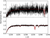 |
Fig. 3. HST/COS G130M spectra of the QSOs VV2006−J131545.2+152556 (upper panel) and PKS2155−304 (lower panel). The COS data are given in black, and the absorber model is plotted in red. Several Lyα absorbers are seen in these spectra. For a better visualisation, both spectra are binned over two pixels. |
The upper panel of Fig. 4 shows the distribution of H I Lyα equivalent widths for the detected absorbers in the two sub-samples and in the combined, total sample. The lower panel shows the distribution of H I column densities in the filament-related absorbers, as derived from the component modelling. Both distributions mimic those seen in previous Lyα studies at z = 0 (Lehner et al. 2007). The sample of Danforth et al. (2016) with 2577 Lyα absorbers obtained with HST/COS shows a similar distribution with a peak in equivalent width just below 100 mÅ. The H I column density distribution falls off below log N(H I) = 13.5 due to the incompleteness in the data regarding the detection of weaker H I Lyα absorbers. We note that, because of the limited spectral resolution and S/N, many of the broader Lyα lines are most likely composed of individual, unresolved sub-components. The H I column density distribution function (CDDF) will be discussed in Sect. 7.
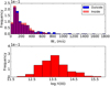 |
Fig. 4. Histogram of equivalent widths of Lyα absorbers (upper panel) and log N(HI) in the filament-related absorbers as derived from the component modelling (lower panel). |
Errors of the measured equivalent widths have been derived with the span code (Richter et al. 2011), which takes into account the S/N around each line, the uncertainty for the local continuum placement, and possible blending effects with other features. Typical 1σ errors for the equivalent widths lie around 20 mÅ. The errors in the column densities were derived based on the component-modelling method in Richter et al. (2011). Here, the typical errors are of the order of ∼0.1 dex.
This value is similar to the errors found by Richter et al. (2017) for the same method and a comparable COS dataset. The Doppler parameters have a relatively high uncertainty, especially for higher values of b. With the majority of b-values falling between 10 and 30 km s−1, the errors are typically ∼5 km s−1, with lower errors for the low end of the range of b and slightly higher errors for larger b-values. Tabulated results from our absorption line measurements can be made available upon request.
4. Characterisation of galaxy filaments
To study how the IGM is connected to its cosmological environment, it is important to characterise the geometry of the filaments, their galaxy content, and their connection to the overall large-scale structure. In Fig. 5, we show the position of the galaxies in the filaments together with their radial extent in 1.5 virial radii (1.5 Rvir). Gas within this characteristic ‘sphere of influence’ can be considered as gravitationally bound to that galaxy. This plot therefore gives a first indication of how much uncovered sky there is between the galaxies and their spheres of influence, indicative of the projected intergalactic space in the filaments (compared to the projected circumgalactic space within 1.5 Rvir). The Virgo Cluster clearly stands out as many galaxies overlap in their projected spheres at 1.5 Rvir, while in most other filaments, there are both regions with strong overlap and regions without overlapping halos. In Sect. 6 and in the appendix, we will discuss other virial radii as selection criteria.
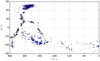 |
Fig. 5. Galaxies belonging to all filaments considered in this study plotted together with their projected 1.5 virial radii. |
4.1. Parametrisation of filament geometry
To define an axis for each filament, a rectangular box was generated per filament containing the galaxies therein. The dark blue filament (see Fig. 2) was split into two individual boxes for geometrical reasons. Widths and lengths of the boxes vary for the different filaments as they scale with the filament’s projected dimensions.
After defining the boxes that sample the individual filaments, they were each sub-divided into segments with the full width of the box and a length corresponding to 20° on the sky. Each segment overlaps with the previous one with half the area (10° length). The average longitude and latitude of the galaxies within each segment was then determined and used as an anchor point to define the filament axis. All these anchor points were connected in each filament to form its axis.
In this way, the definition of the filament axis on the sky allowed us to calculate impact parameters of the COS sightlines to the filaments. In addition, we calculated velocity gradients in the filaments by taking the average velocity of all galaxies in each segment as the velocity anchor point.
The method of using overlapping segments to determine the filament axis is similar to the approach used by Wakker et al. (2015). A difference with their approach is that they first determined which galaxies were part of the filament by looking at the velocities. We did not do this as the filaments were already defined by Courtois et al. (2013). The uncertainty on the placement of the filament axes is no more than 1.5° on the sky, and less for most filaments.
The characteristics of each filament will be discussed separately in the following subsections. The orange or ‘four-cluster’ filament from Courtois et al. (2013) is not discussed here as there are no available COS sightlines nearby.
4.2. Green filament
Perhaps the most notable of the filaments discussed here is the one containing the Virgo Cluster, located at a distance of ∼16.5 Mpc (Mei et al. 2007) and home to as many as 2000 member galaxies. This filament is labelled in green in Fig. 2 and extends from the Centaurus Cluster to the Virgo Cluster in the range l ∼ 260 − 300° and b ∼ 60 − 70°. The Virgo area has the highest galaxy density of the regions studied here.
The axis of the green filament as well as the galaxy velocities are indicated in Fig. 6a. The velocities range from ∼3400 km s−1 at the Centaurus Cluster to ∼ − 400 km s−1. However, the velocities of the galaxies in the Virgo Cluster reach up to ∼2500 km s−1, indicating a large spread in velocities, just as would be expected for a massive galaxy cluster.
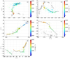 |
Fig. 6. Galaxies belonging to different filaments – (a): green; (b): purple; (c): dark blue; (d): cyan; (e): magenta – with their velocities colour-coded. Grey dots show galaxies belonging to one of the other filaments. The filament axes are indicated with the black solid lines. |
Figure 7 shows that the density along the filament varies greatly, with the Virgo Cluster being the densest region (sub-boxes 6 to 8). In total, this filament has 427 galaxies and 36 COS sightlines passing through it.
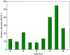 |
Fig. 7. Galaxy density along the green filament. The galaxy density indicates the number of galaxies within 5° on the sky for each galaxy. |
4.3. Purple filament
As mentioned in Courtois et al. (2013), the purple filament is the longest cosmological structure in space among those studied here. In projection, however, it is one of the shorter filaments on the sky. This filament was discussed in detail by Fairall et al. (1998), who named it the ‘Centaurus Wall’. The striking lack of galaxies in the regions around b ∼ 0° evident in Fig. 6b is due to the ZOA caused by the Milky Way disk in the foreground. Just below this scarcely populated region is the Norma Cluster (l ∼ 325°), followed by the Pavus II Cluster (l ∼ 335°).
The purple filament contains the galaxies with the highest velocities in our sample, with v reaching up to 6500 km s−1 (see Fig. 6b). These high velocities indicate distances of ≤85 Mpc. It is the only filament in which the galaxy velocities strongly increase when moving away from Centaurus. As such, it extends beyond the velocity range considered in Courtois et al. (2013). Here, we consider only the part of the filament indicated by their work.
The purple filament is the densest of our defined filaments, which is not surprising as it hosts two galaxy clusters and the projection effect makes it visually compact on the sky. A total of 351 galaxies from the V8k catalogue belong to this filament, though only two COS sightlines, which are both shared with the dark blue filament.
4.4. Dark blue filament
The dark blue filament represents one branch of the Southern Supercluster filament, defined in Courtois et al. (2013). Since it is clearly separated on the sky from the other branch (the cyan filament), these two branches are treated as individual filaments in this study. Starting from the Centaurus Cluster, the dark blue filament is entangled with the purple filament, but it continues to stretch out as a rather diffuse cosmological structure over the range l ∼ 0 − 180° in the southern hemisphere. Because of the low galaxy density, the filament axis of the dark blue filament is not well defined and is unsteady compared to other filaments, as can be seen in Fig. 6c. The dashed portion of the axis indicated in the figure is a result of the small number of galaxies found in this region; as such, the exact filament geometry in this part of the filament remains uncertain.
Figure 6 further indicates that average velocities in the dark blue filament are much lower than in the purple filament, making the two filaments easy to distinguish. The dark blue filament also exhibits two distinct velocity branches – one with velocities ∼2500 km s−1 and one with v ∼ 1300 km s−1 (see Fig. 6) – further underlining the inhomogeneous morphology of this filament. This filament has only 180 galaxies and 21 COS sightlines.
4.5. Cyan filament
The second branch of the Southern Supercluster filament is indicated by the cyan colour in Fig. 2. Compared to the dark blue filament, this branch is rather densely populated and the corresponding filament axis is well defined (Fig. 6d).
As with the green and dark blue filaments, the highest velocities in the cyan filament are found near the Centaurus Cluster, with velocities decreasing as one gets closer to the Fornax Cluster. However, Fig. 6 suggests that there is a slight increase in velocity near the end of the filament at l < 240°. The cyan filament is made up of 289 V8k galaxies, and there are 20 COS sightlines passing though it.
4.6. Magenta filament
This filament (magenta coloured in Fig. 2) contains the Antlia Cluster and also crosses the ZOA. While it is densely populated for b > 0° (near Centaurus), it is under-dense near the ZOA and only moderately populated at negative Galactic latitudes. This makes the transition of the filament axis from positive to negative latitudes hard to define.
As can be seen in Fig. 6e, the velocities in this filament range from 3000 km s−1 near the Centaurus Cluster to 1400 km s−1 near its end at l = 210° and b = −45°. It has 143 galaxies and two usable COS sightlines.
5. Lyα absorption and its connection to galaxies
To learn about the relation between intervening Lyα absorption, nearby galaxies, and the local large-scale structure in which the absorbers and galaxies are embedded, we first looked at the connection between Lyα absorption in the COS data and individual galaxies. In the upper panel of Fig. 8, we plot the equivalent widths of all Lyα absorbers against the line-of-sight impact parameter to the nearest galaxy, ρgal, that has a radial velocity within 400 km s−1 of the absorber. For this plot, all V8k galaxies have been taken into account (not just those in filaments) as some of the absorbers might be related to galaxies outside of the main cosmological structures. We indicate absorbers that are within 1000 km s−1 of the nearest filament in red and those that have larger deviation velocities in blue. Non-detections are indicated by the black crosses. The corresponding sightlines do not show any Lyα absorption in the wavelength range 1220−1243 Å.
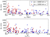 |
Fig. 8. Equivalent width of Lyα absorbers (blue dots) plotted against the impact parameter to the nearest galaxy (upper panel) or against the impact parameter in units of the galaxy’s virial radius (lower panel). The sample has been split into components that lie within 1000 km s−1 of the nearest filament segment (red) and components that have a larger velocity difference (blue). Black crosses indicate sightlines that exhibit no significant Lyα absorption in the analysed spectral region. For these, we give the distance to the nearest galaxy in the velocity range v = 1070 − 6700 km s−1. |
There is an over-density of absorbers within 1 Mpc of the nearest galaxy, many of which have equivalent widths less than Wλ < 200 mÅ. This over-abundance of weak absorbers close to galaxies might be a selection effect. Prominent regions, such as the dense Virgo Cluster, receive more attention by researchers and are sampled by more sightlines (and by spectral data with better S/N) compared to under-dense cosmological regions, which typically are not as well mapped. The highest equivalent widths of the absorbers (Wλ > 500 mÅ) are typically found closer to the galaxies, in line with the often observed anti-correlation between the Lyα equivalent width and the impact parameter (e.g., Chen et al. 2001; French & Wakker 2017). There is, however, a large scatter in this distribution, which has also been seen in other studies (e.g., French & Wakker 2017). This scatter is most likely related to filament regions that have a large galaxy density and overlapping (projected) galaxy halos, as indicated in Fig. 5. Lyα absorption that is detected along a line of sight passing through such a crowded region cannot unambiguously be related to a particular galaxy (such as the nearest galaxy, which is assumed here) but could be associated, with the same likelihood, with any other (e.g., more distant) galaxy and its extended gaseous halo that is sampled by the sightline.
The lower panel of Fig. 8 shows the Lyα equivalent width plotted against ρgal/Rvir. Again, we see the same trend of stronger absorbers being closer to a galaxy. Out of the 208 Lyα absorption components, 29 are within 1.5 virial radii from the nearest galaxy. Following Shull (2014) and Wakker et al. (2015), this is the characteristic radius up to which the gas surrounding a galaxy is immediately associated with that galaxy and its circumgalactic gas-circulation processes (infall, outflows, and mergers). It corresponds to ∼2 − 3 times the gravitational radius as defined in Shull (2014). Outside of this characteristic radius, the gas is more likely associated with the superordinate cosmological environment (i.e. the group or cluster environment and the large-scale filament; but see also Sect. 6 and Fig. B.1). Wakker et al. (2015) use both this distance criterion and the criterion of absorption occurring within 400 km s−1 of the galaxy’s velocity to associate each absorber with either the galaxy or the filament. This velocity range (which we also adopt here; see above) is justified in view of other dynamic processes that would cause a Doppler shift of the gas in relation to the galaxy’s mean radial velocity, such as galaxy rotation, the velocity dispersion of gas structures within the virialised dark-matter of the host galaxy, and in- and outflows.
In Fig. 9, we show how the H I column density (log N(H I)) and the Doppler parameter (b-value) vary with ρgal. Similarly to Wλ, the largest values for log N(H I) and b are found at smaller impact parameters, but (again) the scatter is large.
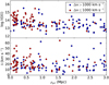 |
Fig. 9. Logarithmic H I column density and the Doppler parameter of Lyα absorbers plotted against ρgal for the same two samples that are shown in Fig. 8. |
Wakker et al. (2015) also plotted the equivalent width versus impact parameter to the nearest galaxy for their sample. Although there are some high equivalent width absorbers at large ρgal (out to 2000 kpc), the average equivalent width decreases with increasing ρgal. Similar to our sample, Wakker et al. (2015) find the majority of the absorbers within 1 Mpc of a galaxy. Our sample, however, has a larger scatter and a larger number of strong absorbers at larger distances. Prochaska et al. (2011) also conclude there is an anti-correlation between equivalent width and the galaxy impact parameter for their sample that has a maximum ρgal of 1 Mpc. In addition to stronger absorbers having lower impact parameters, their sample shows an increase in the number of weak absorbers (Wλ < 100 mÅ) with increasing impact parameter.
6. Lyα and its connection to filaments
In Fig. 10, the filaments are plotted together with the position of the COS sightlines (filled squares) and the velocities of the detected Lyα components, which are colour-coded (in the same way as the galaxies). Only those absorption components that have velocities within 1000 km s−1 of the nearest filament segment are considered. These plots are useful for visualising the large-scale kinematic trends of the absorption features along each filament while also allowing one to explore the spatial and kinematic connection between Lyα components and individual galaxies.
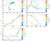 |
Fig. 10. Same as Fig. 6, but here with Lyα absorbers (coloured squares) that fall within 1000 km s−1 of the filament’s velocity overlaid. Multiple absorbers along the same sightline have been given spatial offset. COS sightlines that do not exhibit Lyα absorption in this range are indicated by black crosses |
In the green filament (a), Lyα absorption is predominantly found near 1500 km s−1. This holds true for both the sightlines at the outskirts of the filament and those going through the Virgo Cluster. For the latter, this indicates that the gas has a higher velocity than the typical velocity of galaxies in the Virgo Cluster (as mentioned earlier, the V8k catalogue takes into account the Virgo-flow model by Shaya et al. 1995). Due to the extended Lyα trough in the Galactic foreground ISM absorption, intervening Lyα absorption below ∼1100 km s−1 cannot be measured in our COS dataset, meaning our absorption statistics are incomplete at the low end of the velocity distribution. Still, the trend of decreasing galaxy velocities with increasing distance to the Centaurus Cluster (see above) is not reflected in the kinematics of the detected Lyα absorbers in this filament, which appears to be independent of the large-scale galaxy kinematics.
The purple filament (b) and the first section of the dark blue filament (c) overlap on the sky and have two COS sightlines in common. The different filament velocities allow us to assign the detected Lyα absorption in one of the sightlines to the purple filament, while the other sightline has one absorption component that we associate with the dark blue filament. With only two sightlines available for the purple filament, no clear trends can be identified.
As the dark blue filament continues, the different ‘branches’ noted earlier in Sect. 4.4 are also reflected in the velocities of the Lyα absorption components. This trend might be partly a result of our original selecting criterion for filament-related absorbers (absorption within 1000 km s−1 of the closest filament-segment velocity; see above). However, because of the large velocity range used, the selection criterion cannot account for the entire branching effect. Obviously, in this filament, the gas traces the velocities of the galaxies. Since this is the most diffuse filament, the chance of finding a Lyα absorber that is not directly associated with a galaxy but rather traces the large-scale flow of matter in that filament is higher.
The cyan filament (d) is well populated with galaxies while also being relatively long and broad. It thus has a high cross-section, and there are several sightlines that pass through this structure. Also in this case, the Lyα absorption appears to follow the velocity trend of the galaxies in the filament. Starting from Centaurus, the absorbers first exhibit velocities around 1800 km s−1; the velocities then decrease by several hundred km s−1 to rise again slightly at the end of the filament, in line with the galaxies’ velocity pattern.
Most of the sightlines that pass through the magenta filament (e) are not suited for spectral analysis. The one sightline we analysed shows no significant absorption in the relevant velocity range, implying that no useful information is available for the magenta filament.
Analogous to Fig. 8, Fig. 11 shows the equivalent width of the Lyα absorbers, but now plotted against the filament impact parameter, ρfil. To evaluate whether the absorbers are related to a nearby galaxy, those absorbers that pass within 1.5 Rvir and Δv < 400 km s−1 of a galaxy are shown as open circles, whereas absorbers not associated with a (known) galaxy are indicated with closed circles. In Fig. B.1, we show the effect of varying the impact-parameter criterion on absorbers being associated with a galaxy between 1.0 and 2.5 Rvir (which, however, led to no further insights).
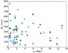 |
Fig. 11. Lyα equivalent width versus filament impact parameter for absorbers with velocities within 1000 km s−1 of the nearest filament segment. Open circles indicate absorbers that are associated with a galaxy (passing it within 1.5 Rvir and Δv < 400 km s−1), and closed circles indicate absorbers that are not associated with a (known) galaxy. The different colours indicate the individual filaments. |
While some of the absorbers with the highest equivalent widths are associated with a galaxy, this is not true for all strong absorbers. Neither sub-sample shows a clear, systematic trend for the equivalent width scaling with ρfil, except that the maximum Lyα equivalent width in a given ρfil bin decreases with increasing distance. However, both sub-samples show a higher absorber density within ρfil < 3 Mpc compared to more distant regions. Some of the absorbers indicated in green extend up to ρfil = 13 Mpc, but these absorbers are unlikely to be part of the green filament as the typical width of a cosmological filament is a few megaparsecs (Bond et al. 2010). But even if we limit our analysis to absorbers with ρfil < 5 Mpc (as in; Wakker et al. 2015), the large scatter in the distribution of Lyα equivalent widths versus the filament impact parameter remains.
The velocity trends for galaxies and absorbers along four filaments (green, purple, dark blue, and cyan) are shown in Fig. 12. The starting point for each filament is the Centaurus Cluster region. Here, each sub-box (segment) is defined to have a length of 10° on the sky. This is half the length of the sub-boxes (segments) used to define the filament axes (see Sect. 4.1) because here, sub-boxes (segments) do not overlap. A length of 20° was only chosen for the second part of the dark blue filament (sub-boxes 12 to 18) in order to have a sufficient number of galaxies available for the determination of a meaningful average velocity.
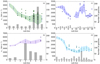 |
Fig. 12. Average galaxy velocities along four filaments (dots) – (a): green; (b): purple; (c): dark blue; (d): cyan – plotted together with the velocities of Lyα absorbers (squares) for each sub-box (segment). The velocity dispersion is indicated by the colour-shaded area. The grey bars indicate the numbers of galaxies belonging to each sub-box (segment) in the filament. |
Both the green and cyan filaments (Figs. 12a and d) show a clear decrease in velocity as they extend farther away from the Centaurus Cluster. For these two filaments, the velocities of the detected Lyα absorbers all lie above the lower limit of the galaxy velocity dispersion in each sub-box, with only one exception (see sub-box 3 in the green filament, where one absorber falls just below the shaded area). This could possibly mean that there is a void of absorbers in the region between the filament and the Milky Way. However, it is important to recall that, because of the Galactic foreground absorption, absorbers with velocities less than ∼1100 km s−1 could not be measured. This limit could also explain why there is no absorption in the lower velocity range of the Virgo Cluster (see sub-boxes 6 and 7 in Fig. 12a).
Furthermore, most absorbers in sub-boxes 2 to 4 and a couple in the other sub-boxes have large ρfil (> 5 Mpc). The velocity spread for those absorbers in the first sub-boxes is larger and trending towards slightly higher velocities than that of the galaxies. Most, however, fall within the standard deviation of the galaxy velocities.
The purple filament contains only three absorbers, all belonging to the same sightline at the end of the filament, as can be seen in Fig. 12b. The plot underlines that this filament is well populated, with more than 50 galaxies in four out of seven sub-boxes.
Just like the filament axis in Fig. 6c, the velocity trend along the dark blue filament is irregular. This trend is also reflected in the absorber velocities. While there are only a few galaxies in each sub-box, the second part of the filament contains 14 absorbers, which is comparable to the total number of absorbers in the cyan filament.
7. Absorber statistics
In quasar-absorption spectroscopy, the observed relation between the number of H I absorption systems in the column density interval ΔN (NH I to NH I + dN) and the absorption path length interval Δx (X to X + dX) is commonly characterised by the differential CDDF, f(NH I). We used the formalism described in Lehner et al. (2007, and references therein) and adopted the following expression to describe the differential CDDF of our Lyα absorbers:
 (1)
(1)
Following, for example, Tytler (1987), absorption path Δx and redshift path Δz at z ≈ 0 can be approximated by the relation
![Mathematical equation: $$ \begin{aligned} \Delta X = 0.5[(1+\Delta z)^2 - 1], \end{aligned} $$](/articles/aa/full_html/2021/03/aa39786-20/aa39786-20-eq3.gif)
where we calculate the redshift path length Δz for the various sightline samples as described in Sect. 3.2. The slope of the CDDF is given by the exponent β, while the normalisation constant, CH I, can be calculated via the relation
![Mathematical equation: $$ \begin{aligned} C_{\rm H\,I } \equiv m_{\rm tot}(1-\beta )/\{N_{\rm max}^{1-\beta } [1-(N_{\rm min}/N_{\rm max})^{1-\beta }]\}. \end{aligned} $$](/articles/aa/full_html/2021/03/aa39786-20/aa39786-20-eq4.gif)
Here, mtot is the total number of absorbers in the column density interval Nmin to Nmax.
The column density distributions for our sample of Lyα absorbers are shown in Fig. 13. The CDDFs were fitted for Lyα components with log N(H I) ≥ 13.2 (maximum log N(H I) = 15.5). For the full filament sightline sample, we derive β = 1.63 ± 0.12, while for the sub-sample of absorbers within 1000 km s−1 of the filament velocity we obtain β = 1.47 ± 0.24. Using high-resolution Space Telescope Imaging Spectrograph (STIS) data, Lehner et al. (2007) derived β = 1.76 ± 0.06 for their sample of narrow absorbers (b ≤ 40 km s−1, 110 absorbers) and β = 1.84 ± 0.06 for b ≤ 150 km s−1 (140 absorbers), thus slightly steeper slopes than the distributions found here. We note that we do not split our sample based on b-values as the fraction of absorbers with b > 40 km s−1 is small (≤5%).
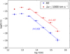 |
Fig. 13. H I CDDF for the Lyα absorbers in sightlines close to filaments (blue) and the absorbers falling within 1000 km s−1 of the filament velocity (red). Errors in log[f(N)] are from Poisson statistics. |
A comparison with other recent studies can be made, for example with the Danforth et al. (2016) COS study of the low-redshift IGM, which yields β = 1.65 ± 0.02 for a redshift-limited sub-sample of 2256 absorbers. Other results are: β = 1.73 ± 0.04 from Danforth & Shull (2008, 650 absorbers from COS), β = 1.65 ± 0.07 by Penton et al. (2000, 187 absorbers from the Goddard High Resolution Spectrograph, GHRS, and STIS), and β = 1.68 ± 0.03 by Tilton et al. (2012, 746 absorbers from STIS). Most of these values are consistent with β = 1.60 − 1.70, whereas higher values (β > 1.70) may indicate a redshift evolution of the slope between z = 0.0 − 0.4. Such an evolution was discussed in Danforth et al. (2016), who find a steepening of the slope with decreasing z in this redshift range. For our study, with z ≤ 0.0223, the slope should be close to the value valid for the universe at z = 0.
Furthermore, the spectral resolution may play a role in the determination of β. For instance, the spectral resolution of COS (R ≈ 20 000) is substantially lower than the resolution of the STIS spectrograph (R ≈ 45 000) used by Lehner et al. (2007); as such, some of our Lyα absorption components might be composed of several (unresolved) sub-components with lower column densities. The limited S/N in the COS data additionally hampers the detection of weak Lyα satellite components in the wings of stronger absorbers (see also Richter et al. 2006a, their Fig. 1).
In this series of results, the shallower CDDF (β = 1.47 ± 0.24) for the sub-sample of velocity-selected absorbers within 1000 km s−1 of the filaments stands out. Although this low value is formally in agreement, within its error range, with the canonical value of β = 1.65, it may hint at a larger relative fraction of high-column-density systems in the filaments, reflecting the spatial concentration of galaxies and the general matter over-density in these structures. A larger sample of Lyα absorbers associated with filaments would be required to further investigate this interesting aspect on a statistically secure basis.
In line with previous studies, our sample offers an opportunity to study the number of Lyα absorbers per unit redshift (d𝒩/dz). Table 1 gives the Lyα line density for the entire sample, as well as for several sub-samples. Those sub-samples separate the sample into different column density bins, allowing us to directly compare the results to the high-resolution Lehner et al. (2007) absorber sample and other studies.
Lyα line density for the full sample (filament- and non-filament-related sightlines), for filament-related sightlines, and for the velocity-selected absorber sample (Δv < 1000 km s−1).
For the full absorber sample (including filament- and non-filament-related sightlines), the Lyα line density is 116 ± 5 lines per unit redshift, but only for the filament-related sub-sample do we have column density information available (see Sect. 3.2). Taking this sub-sample in the ranges 13.2 ≲ log N(H I) ≲ 14.0 and 13.2 ≲ log N(H I) ≲ 16.5, we derive Lyα line densities of 88 ± 8 and 98 ± 8, respectively. These values are in good agreement with those reported by Lehner et al. (2007), who derived number densities of 80 ± 6 and 96 ± 7 for the same column density ranges.
Our results can also be compared with those obtained from the much larger COS absorber sample presented in Danforth et al. (2016). They derive a relation for d𝒩/dz in the form d𝒩(> N)/dz ≈ 25 (N/1014 cm−2)−0.65. For absorbers with log N(H I) ≥ 13.2, this leads to d𝒩/dz ∼ 83, slightly lower than the values derived by us and Lehner et al. (2007), but still in fair agreement.
If we take the velocity-selected absorber sample, which potentially traces the Lyα gas associated with the filaments, we obtain a significantly higher line density of d𝒩/dz = 189 ± 25. The redshift path length for the velocity-selected absorber sample was calculated for each sightline by considering a velocity range of ±1000 km s−1 around the centre velocity for the filament segment that was closest to that sightline.
The value of 189 ± 25 for the velocity-selected filament sample is 93% higher than the value derived for the total filament-absorber sample (along the same lines of sight). This line over-density of the Lyα forest kinematically associated with filaments obviously reflects the matter over-density of baryons in the potential wells of these large-scale cosmological structures.
For the sake of completeness, we also show in Fig. 14 the relation between log N(Si III) and log N(H I) for absorbers in our sample for which both species are detected. Only for a small fraction (8.4%) of the Lyα components can Si III be measured, which is partly because of the velocity-shifted Si III falling in the range of Galactic Lyα absorption. Generally, log N(Si III) increases with log N(H I), as expected from other Si III surveys in the IGM and CGM (e.g., Richter et al. 2016), but the scatter is substantial. The small number of Si III/H I absorbers in our sample does not allow us to draw any meaningful conclusions on the metal content of the absorbers in relation to their large-scale environment.
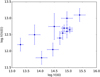 |
Fig. 14. Relation between log N(Si III) and log N(H I) for 13 systems in our absorber sample. |
8. Discussion on Lyα absorbers and their environment
In their study, Prochaska et al. (2011) correlated galaxies and Lyα absorbers at z = 0.06 − 0.57 and found that for weak absorbers (13 ≤ log N(H I) ≤ 14), fewer than 20% of the systems were associated with a known galaxy, while for strong absorbers (log N(H I) ≥ 15), this fraction was 80%. The criteria they used for associating a galaxy with an absorber were the following: (i) a velocity difference between absorber and galaxy of ≤400 km s−1 and (ii) an impact parameter of ρ ≤ 300 kpc. Using the same criteria for our sample, we find that 10% (40%) of the low- (high-) column-density absorbers are associated with a galaxy in the V8k galaxy sample.
Therefore, and in agreement with Prochaska et al. (2011), we find that high-column-density Lyα absorbers are associated four times more often with a galaxy than are low-column-density absorbers; however, the overall percentage of absorbers for which an associated galaxy is found is only half of that in the Prochaska et al. (2011) sample. This can be attributed to the fact that the V8k catalogue is incomplete for MB < −16 and v > 1000 km s−1, while the Prochaska et al. (2011) galaxy sample is complete up to at least z = 0.1 for galaxies with L < 0.1 L*. By comparing their observed covering fractions with a filament model, Prochaska et al. (2011) conclude that all Lyα absorbers are associated with either a galaxy or a filament. This view is debated by Tejos et al. (2012), however, who argue that there is an additional population of ‘random’ Lyα absorbers that reside in the under-dense large-scale structure (voids).
The idea of Lyα absorbers belonging to different populations (and thus different environments) was proposed more than 25 years ago by Morris et al. (1993). By analysing Lyα absorbers in a single sightline and comparing the location of the absorbers with locations of galaxies, these authors found that the absorbers do not cluster around galaxies as strongly as galaxies cluster among themselves. On the other hand, they also found the trend that the absorbers do cluster around galaxies. From this, they concluded that there could be two populations of Lyα absorbers: one that is associated with galaxies and one that is more or less randomly distributed.
To test whether the Lyα absorbers in our sample resemble a ‘random population’, we generated two artificial populations of Lyα absorbers, both with random sky positions, random absorption velocities within the assumed vfil ± 1000 km s−1 velocity range of a filament, and random H I column densities weighted by the H I CDDF. For the first population, we restricted the sample from Lehner et al. (2007, hereafter abbreviated with L07) to the redshift range spanned by the filaments in our study and used the slope of their CDDF (resulting in 39 absorbers, β = 1.76). For the other population, we used our own absorber sample and slope (74 absorbers, β = 1.47). The normalisation constant and absorber path length were calculated using the relations given above. All absorbers were assumed to be at a distance of ≤5 Mpc from the nearest galaxy belonging to a filament, which was also our original criterion to select absorbers inside a filament. The fraction of the simulated absorbers in each filament was adjusted to match the real fractions found in this study. Because the dark blue and purple filaments have an overlap on the sky, their randomised simulated counterparts were generated for both filaments combined.
Figure 15 shows a comparison of how column densities for the three different Lyα absorber samples (observed sample, random sample with own statistics, and random sample with L07 statistics) depend on ρgal. As in Sect. 5, ρgal was calculated for the nearest galaxy on the sky within a velocity interval of 400 km s−1 from the absorber. Clearly, the measured absorbers cluster more strongly around galaxies than either random sample does. This indicates that at least some of the absorbers are associated with galaxies, as expected from previous studies (e.g., Morris & Jannuzi 2006; Prochaska et al. 2011; Tejos et al. 2014; French & Wakker 2017).
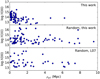 |
Fig. 15. H I column density versus ρgal for Lyα absorbers: as measured in the COS data (upper panel), for a randomised sample following the CDDF in this work (middle panel), and for a randomised sample following the number statistics and CDDF from Lehner et al. (2007, lower panel). |
A very rough estimate of the fraction of absorbers associated with a galaxy can be made by comparing the fraction of absorbers within 1.5 Mpc of a galaxy in different samples. For the measured absorbers, 82% have ρgal ≤ 1.5 Mpc, while the fraction for the randomised sample drawn from our own distribution is 53% and for the L07 random sample it is 46%. In conclusion, about a third of our absorbers cannot be explained by a random population and might be connected to a nearby galaxy.
When comparing the distance of the Lyα absorbers to the nearest filament axis, as shown in Fig. 16, a similar, albeit less pronounced, trend can be seen. Measured absorbers are generally found closer to the filament axis than a random distribution shows. One may argue that this could be a selection effect, for example from targeting particularly interesting areas such as the Virgo Cluster, which would result in more sightlines near the Virgo filament. However, Fig. 11 shows the breakdown of absorbers into different filaments, demonstrating that the absorbers belonging to the Virgo Cluster filament (green) are in fact more spread out than absorbers in other regions, disproving such a selection effect.
To further investigate the possible clustering signal of Lyα absorbers near the filament axis, we plot, in Fig. 17, the cumulative distribution function for ρfil for the three previously mentioned absorber samples (observed sample, random sample with own statistics, and random sample with L07 statistics) as well as the galaxies that constitute the filament. We have also added another absorber test sample (D16) generated from the Lyα column density distribution of absorbers reported in Danforth et al. (2016). The cumulative distribution of galaxies sets the reference point as these define the filament. As can be seen, the observed distribution of absorbers clusters more strongly around the filament axis than do the three random absorber test distributions, but not as strongly as the galaxies. Within the inner 2 Mpc, in particular, the fraction of measured Lyα absorbers rises faster than the synthetic absorbers in the randomised samples.
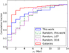 |
Fig. 17. Cumulative distribution function for ρfil for three different absorber samples. The measured absorbers in the COS data are indicated in blue, the random sample with its own statistics is plotted in dashed green, the random sample with the L07 statistics is indicated in dotted black, and the random sample from Danforth et al. (2016) is added in dashed magenta (D16). The distribution for the galaxies is shown in red. |
The cumulative distribution function as shown in Fig. 17 can be compared with that for absorbers associated with galaxies. Figure 3 in Penton et al. (2002) shows this function for 46 Lyα absorbers and sub-samples thereof. Their full sample follows a distribution similar to that of our absorbers, with ∼60% found within 2 Mpc of the nearest galaxy (Penton et al. 2002) or filament (this study). Both studies show the galaxies more strongly clustered than the Lyα absorbers. Stocke et al. (2013) compared their absorber-galaxy cumulative distribution function with a random distribution and concluded that absorbers are associated with galaxies in a more general way, namely, they trace the large-scale structure instead of individual galaxies. Penton et al. (2002), Stocke et al. (2013), and Keeney et al. (2018) all conclude that high-column-density absorbers are more strongly correlated with galaxies than those with lower column densities. This is in agreement with what is found here: Lyα absorbers do not trace the same distribution as galaxies, but they are not randomly distributed around filaments either.
Kolmogorov–Smirnov test for impact-parameter distributions.
A Kolmogorov–Smirnov (KS) test confirms that the absorbers found in the COS data are not drawn from a random distribution. Table 2 lists the KS values and p-values for the different samples.
A KS test can be used to compare two different samples to evaluate whether or not they are drawn from the same parent distribution. A high KS value (maximum of 1) indicates a high probability that this is true. The p-value instead indicates the significance that the null hypothesis is rejected. In this case, the null hypothesis is that ρfil for the absorbers measured in this study follows the same distribution as that of a random sample or of the galaxies in the filament. A p-value of < 0.05 means that the null hypothesis can be rejected with a probability of > 95%. In all three comparisons between the measurements and the random absorber samples (our own sample, randomised, and the randomised L07 and D16 samples), the KS test indicates that they do not follow the same distribution.
The low p-value that we obtain from comparing the COS absorber sample with the V8k galaxy sample in the filaments further indicates that the Lyα absorbers are not drawn from the same distribution as the galaxies. To evaluate the hypothesis that there are two populations of Lyα absorbers (e.g., Morris et al. 1993; Tejos et al. 2012), we removed from the sample (as a test) those absorbers that we had associated with galaxies. This had, however, no significant effect on the cumulative distribution function for ρfil.
In conclusion, the cumulative distribution functions for ρfil show that galaxies are more strongly clustered in the filaments than are the Lyα absorbers that belong to the same cosmological structures. Lyα absorbers do not follow a random distribution, nor do they follow the same distribution as the galaxies that constitute large-scale filaments. There might be two (or more) separate populations of Lyα absorbers in filaments, but there is no evidence (from our study) that the Lyα absorbers that are not directly associated with large galaxies are randomly distributed in the field of the filament.
Deeper insights into these aspects (including other important cosmological issues such as over-density bias factors and how they affect the absorber-to-galaxy-to-filament statistics) are highly desirable. However, they will require a much larger observational dataset in combination with numerical cosmological simulations.
9. Summary and concluding remarks
In this study, we have combined galaxy data of more than 30 000 nearby galaxies from the V8k catalogue Courtois et al. (2013) with HST/COS UV spectral data of 302 distant AGN to investigate the relation between intervening H I Lyα absorbers and five nearby cosmological structures (galaxy filaments) at z ≈ 0 (v < 6700 km s−1).
(1) All in all, we identify 587 intervening Lyα absorbers along the 302 COS sightlines in the wavelength range between 1220 and 1243 Å. For the 91 sightlines that pass through the immediate environment of the examined galaxy filaments, we analysed 215 (227) Lyα absorption systems (components) in detail and derived column densities and b-values for H I (and associated metals, if available).
(2) For the individual galaxies in our sample, we have calculated the virial radii from their luminosities and the galaxy impact parameters, ρgal, to the COS sightlines. We assume 29 Lyα absorbers to be directly associated with galaxies as they are located within 1.5 virial radii of their host galaxies and within 400 km s−1 of the galaxies’ recession velocity.
(3) We characterise the geometry of the galaxy filament by considering the galaxy distribution in individual segments of the filaments. In this way, we define for each filament a geometrical axis that we use as reference for defining the filament impact parameters, ρfil, for those Lyα absorbers that are located within 1000 km s−1 of the filament.
(4) We find that the absorption velocities of the Lyα absorbers reflect the large-scale velocity pattern of the four galaxy filaments, for which sufficient absorption line data are available. Seventy-four absorbers are aligned in position and velocity with the galaxy filaments, indicating that these absorbers and the galaxies trace the same large-scale structure.
(5) If we relate the measured Lyα equivalent widths (or H I column densities) with the galaxy and filament impact parameters, we find that the strongest absorbers (equivalent widths Wλ > 500 mÅ) are preferentially located in the vicinity of individual galaxies (within 3 virial radii) and/or in the vicinity of the filament axes (within 5 Mpc). The observed relations between W and ρgal/ρfil exhibit substantial scatter, however, disfavouring a simple equivalent width with impact parameter anti-correlation.
(6) We find that the measured H I components follow a CDDF with a slope of −β = −1.63 ± 0.12, a value that is typical for the low-redshift Lyα forest. Only for the sub-sample of absorbers within 1000 km s−1 of the filament velocity do we obtain a shallower CDDF with β = 1.47 ± 0.24, possibly indicating an excess of high-column-density absorbers in galaxy filaments when compared to the overall Lyα forest.
(7) The Lyα absorbers that lie within 1000 km s−1 of the nearest filament have a ∼90% higher rate of incidence (d𝒩/dz = 189 ± 25 for log N(H I) ≥ 13.2) than that of the general Lyα absorber population in our sample (d𝒩/dz = 98 ± 8 for log N(H I) ≥ 13.2). This higher number density of Lyα absorbers per unit redshift most likely reflects the filaments’ general matter over-density.
(8) We compare the filament impact-parameter distributions of the galaxies, measured Lyα absorbers, and a (synthetic) Lyα absorber sample with randomised locations on the sky with one another. We find that the galaxies are most strongly clustered around the filament axes, while the spatial clustering of the observed Lyα absorbers around the filament axes is evident but less pronounced. Using a KS test, we confirm that the Lyα absorbers neither follow the impact-parameter distribution of the galaxies nor a random distribution, but represent an individual, spatially confined sample of objects.
Taken together, the results of our study underline that the relation between intervening Lyα absorbers, large-scale cosmological filaments, and individual galaxies (that constitute the filaments) in the local universe is complex and manifold, and difficult to reconstruct with existing data.
This complexity is not surprising, of course, if we recall what Lyα absorbers actually are: They are objects that trace local gas over-densities in an extremely extended, diffuse medium that is gravitationally confined in hierarchically structured potential wells and stirred up by large-scale matter flows and galaxy feedback. In this picture, the spatial distribution of Lyα absorbers in cosmological filaments is governed by both the distribution of individual sinks in the large-scale gravitational potential energy distribution (i.e. galaxies, galaxy groups, etc.) and more (or less) stochastically distributed density fluctuations at larger scales that reflect the internal dynamics of the IGM.
For the future, we are planning to extend our study of the relation between intervening absorbers and cosmological filaments in the local universe. We will use a larger (and deeper) galaxy sample and additional HST/COS spectra, in combination with constrained magneto-hydrodynamic cosmological simulations of nearby cosmological structures.
Throughout the following, we use the expression “QSO” as synonym for all types of AGN.
Acknowledgments
The authors would like to thank the referee for his valuable comments and suggestions which helped to improve the manuscript.
References
- Bond, N. A., Strauss, M. A., & Cen, R. 2010, MNRAS, 409, 156 [NASA ADS] [CrossRef] [Google Scholar]
- Bowen, D. V., Pettini, M., & Blades, J. C. 2002, ApJ, 580, 169 [NASA ADS] [CrossRef] [Google Scholar]
- Bower, R. G., Benson, A. J., Malbon, R., et al. 2006, MNRAS, 370, 645 [NASA ADS] [CrossRef] [Google Scholar]
- Cen, R., & Ostriker, J. P. 1999, ApJ, 514, 1 [NASA ADS] [CrossRef] [Google Scholar]
- Chen, H.-W., Lanzetta, K. M., Webb, J. K., & Barcons, X. 2001, ApJ, 559, 654 [NASA ADS] [CrossRef] [Google Scholar]
- Colless, M., Dalton, G., Maddox, S., et al. 2001, MNRAS, 328, 1039 [NASA ADS] [CrossRef] [Google Scholar]
- Courtois, H. M., Pomarède, D., Tully, R. B., Hoffman, Y., & Courtois, D. 2013, AJ, 146, 69 [NASA ADS] [CrossRef] [Google Scholar]
- Danforth, C. W., & Shull, J. M. 2008, ApJ, 679, 194 [NASA ADS] [CrossRef] [Google Scholar]
- Danforth, C. W., Keeney, B. A., Tilton, E. M., et al. 2016, ApJ, 817, 111 [NASA ADS] [CrossRef] [Google Scholar]
- Dashtamirova, D., & Fischer, W. J. 2018, Cosmic Origins Spectrograph Instrument Handbook, Version 12.0 (Baltimore: STScI) [Google Scholar]
- Davé, R., Hernquist, L., Katz, N., & Weinberg, D. H. 1999, ApJ, 511, 521 [NASA ADS] [CrossRef] [Google Scholar]
- Davies, J. J., Crain, R. A., McCarthy, I. G., et al. 2019, MNRAS, 485, 3783 [NASA ADS] [CrossRef] [Google Scholar]
- Erb, D. K. 2008, ApJ, 674, 151 [NASA ADS] [CrossRef] [Google Scholar]
- Fairall, A. P., Woudt, P. A., & Kraan-Korteweg, R. C. 1998, A&AS, 127, 463 [NASA ADS] [CrossRef] [EDP Sciences] [Google Scholar]
- French, D. M., & Wakker, B. P. 2017, ApJ, 837, 138 [NASA ADS] [CrossRef] [Google Scholar]
- Genzel, R., Tacconi, L. J., Gracia-Carpio, J., et al. 2010, MNRAS, 407, 2091 [Google Scholar]
- Green, J. C., Froning, C. S., Osterman, S., et al. 2012, ApJ, 744, 60 [NASA ADS] [CrossRef] [Google Scholar]
- Keeney, B. A., Stocke, J. T., Pratt, C. T., et al. 2018, ApJS, 237, 11 [NASA ADS] [CrossRef] [Google Scholar]
- Lehner, N., Savage, B. D., Richter, P., et al. 2007, ApJ, 658, 680 [NASA ADS] [CrossRef] [Google Scholar]
- Madau, P., Ferrara, A., & Rees, M. J. 2001, ApJ, 555, 92 [NASA ADS] [CrossRef] [Google Scholar]
- Martizzi, D., Vogelsberger, M., Artale, M. C., et al. 2019, MNRAS, 486, 3766 [Google Scholar]
- Mei, S., Blakeslee, J. P., Côté, P., et al. 2007, ApJ, 655, 144 [NASA ADS] [CrossRef] [Google Scholar]
- Morris, S. L., & Jannuzi, B. T. 2006, MNRAS, 367, 1261 [Google Scholar]
- Morris, S. L., Weymann, R. J., Dressler, A., et al. 1993, ApJ, 419, 524 [NASA ADS] [CrossRef] [Google Scholar]
- Morton, D. C. 2003, ApJS, 149, 205 [NASA ADS] [CrossRef] [MathSciNet] [Google Scholar]
- Pallottini, A., Gallerani, S., & Ferrara, A. 2014, MNRAS, 444, L105 [NASA ADS] [CrossRef] [Google Scholar]
- Penton, S. V., Shull, J. M., & Stocke, J. T. 2000, ApJ, 544, 150 [NASA ADS] [CrossRef] [Google Scholar]
- Penton, S. V., Stocke, J. T., & Shull, J. M. 2002, ApJ, 565, 720 [NASA ADS] [CrossRef] [Google Scholar]
- Prochaska, J. X., & Wolfe, A. M. 2009, ApJ, 696, 1543 [NASA ADS] [CrossRef] [Google Scholar]
- Prochaska, J. X., Weiner, B., Chen, H. W., Mulchaey, J., & Cooksey, K. 2011, ApJ, 740, 91 [Google Scholar]
- Richter, P., Fang, T., & Bryan, G. L. 2006a, A&A, 451, 767 [NASA ADS] [CrossRef] [EDP Sciences] [Google Scholar]
- Richter, P., Savage, B. D., Sembach, K. R., & Tripp, T. M. 2006b, A&A, 445, 827 [NASA ADS] [CrossRef] [EDP Sciences] [Google Scholar]
- Richter, P., Paerels, F. B. S., & Kaastra, J. S. 2008, Space Sci. Rev., 134, 25 [NASA ADS] [CrossRef] [Google Scholar]
- Richter, P., Krause, F., Fechner, C., Charlton, J. C., & Murphy, M. T. 2011, A&A, 528, A12 [NASA ADS] [CrossRef] [EDP Sciences] [Google Scholar]
- Richter, P., Fox, A. J., Wakker, B. P., et al. 2013, ApJ, 772, 111 [NASA ADS] [CrossRef] [Google Scholar]
- Richter, P., Wakker, B. P., Fechner, C., et al. 2016, A&A, 590, A68 [NASA ADS] [CrossRef] [EDP Sciences] [Google Scholar]
- Richter, P., Nuza, S. E., Fox, A. J., et al. 2017, A&A, 607, A48 [NASA ADS] [CrossRef] [EDP Sciences] [Google Scholar]
- Saunders, W., d’Mellow, K. J., Tully, R. B., et al. 2000a, in Mapping the Hidden Universe: The Universe behind the Mily Way – The Universe in HI, eds. R. C. Kraan-Korteweg, P. A. Henning, & H. Andernach, ASP Conf. Ser., 218, 153 [Google Scholar]
- Saunders, W., Sutherland, W. J., Maddox, S. J., et al. 2000b, MNRAS, 317, 55 [NASA ADS] [CrossRef] [Google Scholar]
- Shaya, E. J., Peebles, P. J. E., & Tully, R. B. 1995, ApJ, 454, 15 [NASA ADS] [CrossRef] [Google Scholar]
- Shull, J. M. 2003, in The IGM/Galaxy Connection. The Distribution of Baryons at z=0, eds. J. L. Rosenberg, & M. E. Putman, Astrophys. Space Sci. Lib., 281, 1 [Google Scholar]
- Shull, J. M. 2014, ApJ, 784, 142 [NASA ADS] [CrossRef] [Google Scholar]
- Shull, J. M., Smith, B. D., & Danforth, C. W. 2012, ApJ, 759, 23 [NASA ADS] [CrossRef] [Google Scholar]
- Stocke, J. T., Keeney, B. A., Danforth, C. W., et al. 2013, ApJ, 763, 148 [Google Scholar]
- Tejos, N., Morris, S. L., Crighton, N. H. M., et al. 2012, MNRAS, 425, 245 [Google Scholar]
- Tejos, N., Morris, S. L., Finn, C. W., et al. 2014, MNRAS, 437, 2017 [Google Scholar]
- Tejos, N., Prochaska, J. X., Crighton, N. H. M., et al. 2016, MNRAS, 455, 2662 [NASA ADS] [CrossRef] [Google Scholar]
- Tilton, E. M., Danforth, C. W., Shull, J. M., & Ross, T. L. 2012, ApJ, 759, 112 [NASA ADS] [CrossRef] [Google Scholar]
- Tully, R. B., Rizzi, L., Shaya, E. J., et al. 2009, ArXiv e-prints [arXiv:0902.3668] [Google Scholar]
- Tumlinson, J., Shull, J. M., Rachford, B. L., et al. 2002, ApJ, 566, 857 [NASA ADS] [CrossRef] [Google Scholar]
- Tytler, D. 1987, ApJ, 321, 49 [NASA ADS] [CrossRef] [Google Scholar]
- Wakker, B. P., & Savage, B. D. 2009, ApJS, 182, 378 [NASA ADS] [CrossRef] [Google Scholar]
- Wakker, B. P., Hernandez, A. K., French, D. M., et al. 2015, ApJ, 814, 40 [NASA ADS] [CrossRef] [Google Scholar]
- York, D. G., Adelman, J., Anderson, J. E., Jr., et al. 2000, AJ, 120, 1579 [CrossRef] [Google Scholar]
Appendix A: Signal-to-noise
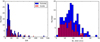 |
Fig. A.1. Information on the S/N of the COS spectra used in this study. Left panel: distribution of the measured S/N per resolution element near Å 1240 for the COS spectra that are filament-related and those outside of filaments. Right panel: formal 3σ detection limits for H I Ly α absorption in these spectra, based on the equation given in Tumlinson et al. (2002). We note that these values reflect the detectability of Ly α absorption as a function of the local S/N under idealised conditions (no blending, no fixed-pattern noise, perfectly known continuum flux). |
Appendix B: Absorbers associated with galaxies
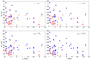 |
Fig. B.1. Same as Fig. 11, but now using different impact-parameter criteria, ρgal, for absorbers to be associated with a galaxy. Filled blue dots are absorbers associated with a galaxy, while open red dots are absorbers that are not. |
All Tables
Lyα line density for the full sample (filament- and non-filament-related sightlines), for filament-related sightlines, and for the velocity-selected absorber sample (Δv < 1000 km s−1).
All Figures
|
Fig. 1. Histogram of apparent and absolute B-band magnitudes and luminosities for all galaxies of the V8k catalogue. |
| In the text | |
|
Fig. 2. All-sky map of filaments in the local Universe. Upper panel: sky distribution of galaxies from V8k belonging to filaments as defined in Courtois et al. (2013). The different colours indicate different galaxy filaments. Several important clusters are noted. Lower panel: sky distribution of HST/COS sightlines passing close to a filament (black circles) and HST/COS sightlines not belonging to a filament (grey circles) plotted together with the galaxies from the V8k catalogue belonging to filaments (colour-coded according to velocity). |
| In the text | |
|
Fig. 3. HST/COS G130M spectra of the QSOs VV2006−J131545.2+152556 (upper panel) and PKS2155−304 (lower panel). The COS data are given in black, and the absorber model is plotted in red. Several Lyα absorbers are seen in these spectra. For a better visualisation, both spectra are binned over two pixels. |
| In the text | |
|
Fig. 4. Histogram of equivalent widths of Lyα absorbers (upper panel) and log N(HI) in the filament-related absorbers as derived from the component modelling (lower panel). |
| In the text | |
|
Fig. 5. Galaxies belonging to all filaments considered in this study plotted together with their projected 1.5 virial radii. |
| In the text | |
|
Fig. 6. Galaxies belonging to different filaments – (a): green; (b): purple; (c): dark blue; (d): cyan; (e): magenta – with their velocities colour-coded. Grey dots show galaxies belonging to one of the other filaments. The filament axes are indicated with the black solid lines. |
| In the text | |
|
Fig. 7. Galaxy density along the green filament. The galaxy density indicates the number of galaxies within 5° on the sky for each galaxy. |
| In the text | |
|
Fig. 8. Equivalent width of Lyα absorbers (blue dots) plotted against the impact parameter to the nearest galaxy (upper panel) or against the impact parameter in units of the galaxy’s virial radius (lower panel). The sample has been split into components that lie within 1000 km s−1 of the nearest filament segment (red) and components that have a larger velocity difference (blue). Black crosses indicate sightlines that exhibit no significant Lyα absorption in the analysed spectral region. For these, we give the distance to the nearest galaxy in the velocity range v = 1070 − 6700 km s−1. |
| In the text | |
|
Fig. 9. Logarithmic H I column density and the Doppler parameter of Lyα absorbers plotted against ρgal for the same two samples that are shown in Fig. 8. |
| In the text | |
|
Fig. 10. Same as Fig. 6, but here with Lyα absorbers (coloured squares) that fall within 1000 km s−1 of the filament’s velocity overlaid. Multiple absorbers along the same sightline have been given spatial offset. COS sightlines that do not exhibit Lyα absorption in this range are indicated by black crosses |
| In the text | |
|
Fig. 11. Lyα equivalent width versus filament impact parameter for absorbers with velocities within 1000 km s−1 of the nearest filament segment. Open circles indicate absorbers that are associated with a galaxy (passing it within 1.5 Rvir and Δv < 400 km s−1), and closed circles indicate absorbers that are not associated with a (known) galaxy. The different colours indicate the individual filaments. |
| In the text | |
|
Fig. 12. Average galaxy velocities along four filaments (dots) – (a): green; (b): purple; (c): dark blue; (d): cyan – plotted together with the velocities of Lyα absorbers (squares) for each sub-box (segment). The velocity dispersion is indicated by the colour-shaded area. The grey bars indicate the numbers of galaxies belonging to each sub-box (segment) in the filament. |
| In the text | |
|
Fig. 13. H I CDDF for the Lyα absorbers in sightlines close to filaments (blue) and the absorbers falling within 1000 km s−1 of the filament velocity (red). Errors in log[f(N)] are from Poisson statistics. |
| In the text | |
|
Fig. 14. Relation between log N(Si III) and log N(H I) for 13 systems in our absorber sample. |
| In the text | |
|
Fig. 15. H I column density versus ρgal for Lyα absorbers: as measured in the COS data (upper panel), for a randomised sample following the CDDF in this work (middle panel), and for a randomised sample following the number statistics and CDDF from Lehner et al. (2007, lower panel). |
| In the text | |
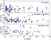 |
Fig. 16. Same as Fig. 15, but now for ρfil. |
| In the text | |
|
Fig. 17. Cumulative distribution function for ρfil for three different absorber samples. The measured absorbers in the COS data are indicated in blue, the random sample with its own statistics is plotted in dashed green, the random sample with the L07 statistics is indicated in dotted black, and the random sample from Danforth et al. (2016) is added in dashed magenta (D16). The distribution for the galaxies is shown in red. |
| In the text | |
|
Fig. A.1. Information on the S/N of the COS spectra used in this study. Left panel: distribution of the measured S/N per resolution element near Å 1240 for the COS spectra that are filament-related and those outside of filaments. Right panel: formal 3σ detection limits for H I Ly α absorption in these spectra, based on the equation given in Tumlinson et al. (2002). We note that these values reflect the detectability of Ly α absorption as a function of the local S/N under idealised conditions (no blending, no fixed-pattern noise, perfectly known continuum flux). |
| In the text | |
|
Fig. B.1. Same as Fig. 11, but now using different impact-parameter criteria, ρgal, for absorbers to be associated with a galaxy. Filled blue dots are absorbers associated with a galaxy, while open red dots are absorbers that are not. |
| In the text | |
Current usage metrics show cumulative count of Article Views (full-text article views including HTML views, PDF and ePub downloads, according to the available data) and Abstracts Views on Vision4Press platform.
Data correspond to usage on the plateform after 2015. The current usage metrics is available 48-96 hours after online publication and is updated daily on week days.
Initial download of the metrics may take a while.