| Issue |
A&A
Volume 647, March 2021
|
|
|---|---|---|
| Article Number | A30 | |
| Number of page(s) | 12 | |
| Section | Numerical methods and codes | |
| DOI | https://doi.org/10.1051/0004-6361/202039626 | |
| Published online | 04 March 2021 | |
Synthesising the repeating FRB population using frbpoppy
1
ASTRON, the Netherlands Institute for Radio Astronomy, Oude Hoogeveensedijk 4, 7991 PD Dwingeloo, The Netherlands
e-mail: This email address is being protected from spambots. You need JavaScript enabled to view it.
2
Anton Pannekoek Institute for Astronomy, University of Amsterdam, Science Park 904, 1098 XH Amsterdam, The Netherlands
Received:
9
October
2020
Accepted:
9
December
2020
Abstract
The observed fast radio burst (FRB) population can be divided into one-off and repeating FRB sources. Either this division is a true dichotomy of the underlying sources, or selection effects and low activity prohibit us from observing repeat pulses from all constituents making up the FRB source population. We attempted to break this degeneracy through FRB population synthesis. With that aim in mind, we extended frbpoppy (which previously only handled one-off FRBs) to also simulate repeaters. We next modelled the Canadian Hydrogen Intensity Mapping Experiment FRB survey (CHIME/FRB). Using this implementation, we investigated the impact of luminosity functions on the observed dispersion measure (DM) and distance distributions of both repeating and one-off FRBs. We show that for a single, intrinsically repeating source population with a steep luminosity function, selection effects should shape the DM distributions of one-off and repeating FRB sources differently. This difference is not yet observed. We next show how the repeater fraction over time can help in determining the repetition rate of an intrinsic source population. We simulated this fraction for CHIME/FRB, and we show that a source population comprised solely of repeating FRBs can describe CHIME/FRB observations with the use of a flat luminosity function. From the outcome of these two methods, we thus conclude that all FRBs originate from a single and mostly uniform population of varying repeaters. Within this population, the luminosity function cannot be steep, and there must be minor differences in physical or behaviour parameters that correlate with the repetition rate.
Key words: radio continuum: general / methods: statistical
© ESO 2021
1. Introduction
Fast radio bursts (FRBs) are millisecond-long pulses detected at radio frequencies (Cordes & Chatterjee 2019; Petroff et al. 2019). As of now (Petroff & Chatterjee 2020), at least 21 FRB sources have been observed to repeat (repeaters), with 127 FRB sources not having been observed to repeated (one-offs). Originally, FRBs were serendipitously observed by pulsar surveys, but dedicated FRB surveys began in 2018. The three main observatories searching for FRBs include the Canadian Hydrogen Intensity Mapping Experiment (CHIME; CHIME/FRB Collaboration 2018), the Australian Square Kilometre Array Pathfinder (ASKAP; Macquart et al. 2010; Johnston et al. 2007), and Apertif on Westerbork (Maan & van Leeuwen 2017; van Leeuwen et al. in prep.). While initially each new FRB detection was considered newsworthy (e.g. Masui et al. 2015), the rise in FRB detections through these FRB surveys has ushered in the dawn of FRB population studies (Macquart et al. 2019). Initial population studies had few FRBs with which to work (Thornton et al. 2013; Macquart & Johnston 2015); however, subsequent studies investigating detection biases (Macquart & Ekers 2018b), rate distributions (James et al. 2020), or spectral properties (Macquart et al. 2019) were able to utilise a larger sample of FRBs.
The detection of a repeating FRB source in 2016 (Spitler et al. 2016) raised the question of whether all FRB sources repeat. Do both apparent types of FRBs emerge from the same intrinsic source population? Despite extensive observational campaigns (e.g. Petroff et al. 2015; Shannon et al. 2018), no conclusive evidence has emerged either way. Theoretical studies of possible FRB source mechanisms provide no conclusive answer either. Models such as neutron star–white dwarf accretion (Gu et al. 2016), supergiant pulses (Cordes & Wasserman 2016), blast waves from magnetars (Metzger et al. 2019), or emission within neutron star magnetospheres (Lyutikov & Popov 2020) can produce both repeaters and one-offs.
One possible approach to probing the intrinsic source class is population synthesis. In studies of pulsars (Taylor & Manchester 1977), gamma-ray bursts (Ghirlanda et al. 2013), and stellar evolution (Izzard & Halabi 2018), population synthesis has proven to be a powerful tool. To this end, we previously implemented an open-source FRB POPulation sythesis package in PYthon (frbpoppy; Gardenier et al. 2019). This first version was capable of modelling one-off FRBs and successfully reproducing the observed one-off FRB populations as seen by the High Time Resolution Universe (HTRU) survey and by ASKAP. In this paper, we present an updated version of frbpoppy capable of modelling repeating FRB sources. We use it to probe the intrinsic FRB source population in multiple ways. These methods could allow the field to determine the nature of the FRB population.
Prior population synthesis efforts by Caleb et al. (2019) simulated repeaters with a variety of wait time distributions to determine expected detection rates and constraints on the slope of the intrinsic energy distribution. frbpoppy takes a different approach, with increased focus on survey modelling to replicate a wide range of selection effects. Additionally, frbpoppy was designed from the start to be an open source, modular Python package for easy use by the community (Gardenier et al. 2019). Simulations of the repeating FRB population are increasingly being used to probe various aspects of the intrinsic FRB population (e.g. Ai et al. 2021), but they often lack the modelling of the full range selection effects present in the observed FRB population, which are essential.
In this paper, we use population synthesis to show several methods by which the intrinsic FRB source population can be constrained. We begin by detailing our approach to synthesising a repeating FRB population, before providing our results and interpretation in the second half. As such, we present an implementation of repeating sources in Sect. 2, which covers both the generation and surveying of repeating sources. In Sect. 3, we show several ways that population synthesis identifies selection effects in the observed FRB populations, through which the intrinsic FRB source population can be probed. We subsequently summarise our thoughts in Sect. 4. The paper ends with Appendix A, which contains information relevant to our methods.
2. Simulating a repeater population
Population synthesis is a method by which properties of an underlying, real source population are derived by simulating virtual populations (see e.g. Taylor & Manchester 1977). To this end, we presented frbpoppy in Gardenier et al. (2019): a code base capable of modelling one-off FRBs, and thus constraining properties of the intrinsic FRB source population. Additional constraints on the FRB source population can, however, be found by looking at repeating FRB sources (see e.g. Fonseca et al. 2020). We aim to take advantage of repeater observations by incorporating repeating sources into frbpoppy. These features can be found in the v2 release of frbpoppy, accessible on Github1.
Shifting from one-off FRB sources to repeating sources requires additional frbpoppy functionalities in three major areas: simulating burst times, generating properties, and surveying populations. This functionality is described in the following sections. In describing such population synthesis methods, the term ‘observed population’ can be confusing as there are both real and simulated observed populations. The interpretation can often be gained from the context, but where this is lacking, we ensure the terms, real or simulated, are added. Furthermore, the term FRB originally referred to both the burst and the source. For repeaters, these are different concepts. Throughout this paper, we use ‘burst’ to refer to an individual flash of light, and ‘source’ to refer to an origin of these bursts. We thus use the term FRB to refer to a single burst. To distinguish software input from other connotations, we use a recognisable typeface, for example chime-frb, as an argument over CHIME/FRB the survey.
2.1. Generating burst times
Where simulations of one-off FRBs can be relatively static, repeaters require the simulation of repetition. In frbpoppy, we generate a series of burst time stamps per FRB source. A variety of distributions can be used to generate these time stamps, including the following:
single: to simulate one-off sources, the single option generates a single time interval per source within a given time frame:
 (1)
(1)
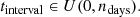
Here, time intervals (tinterval) are drawn from a uniform distribution U in the range zero to the chosen maximum number of days ndays.
regular: to replicate pulsars (Hewish et al. 1968), and for testing purposes, we allow for perfectly regular time intervals:
 (2)
(2)
with rate r and integer k, an iterator ensuring the maximum value of tinterval remains smaller than the maximum timescale (ndays). The rate r can vary per source.
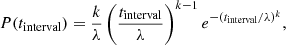
poisson: we can draw bursts from a Poissonian distribution, similar to the giant-pulse behaviour in pulsars (Lundgren et al. 1995). We use the inverse cumulative distribution function (CDF) of an exponential function. In this case, the probability density function (PDF) can be described as
 (3)
(3)
for the rate r when r ≥ 0. From this, the inverse CDF can be derived:
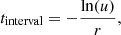 (4)
(4)
with rate r and u ∈ U(0, 1), where U represents a uniform distribution. To ensure enough bursts are simulated per source, they are drawn per FRB source until the cumulative time interval would result in a burst beyond the requested maximum timescale (ndays). This last time interval is subsequently masked. To simulate a variety of FRB sources, the rate r can be chosen to vary per source.
clustered: as FRB121102 follows a distinctly non-Poissonian burst rate (Oppermann et al. 2018), frbpoppy can simulate such clustered bursts. Time intervals are now drawn from the inverse CDF of the Weibull distribution. The PDF of a Weibull distribution can be described as
 (5)
(5)
with the following scale parameter:
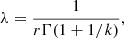 (6)
(6)
and the gamma function Γ, shape parameter k, and rate parameter r for tinterval ≥ 0, from which the inverse CDF can be derived:
 (7)
(7)
with the rate parameter r, gamma function Γ, shape parameter k, and u ∈ U(0, 1) with uniform distribution U. Just as with the poisson option, bursts are iteratively generated up to the maximum timescale (ndays).
cyclic: with several repeaters showing quasi-periodic activity (see Bochenek et al. 2020; Rajwade et al. 2020; Cruces et al. 2020), the cyclic option allows frbpoppy to model bursts emerging during an active window. For simplicity, we modelled the arrival times of bursts during the active window as a uniform distribution:
 (8)
(8)
with nactive the number of active days per activity cycle of the source. The number of generated bursts is given by the product of the number of bursts per active period and the number of activity cycles within the maximum timescale (ndays):
 (9)
(9)
with a burst rate r and an activity cycle of P days. For each next activity cycle, a whole period is added to the generated burst time to convert them into time stamps between 0 and ndays.
To generate time stamps from the time intervals given in some of these distributions, we took cumulative time intervals per source:
 (10)
(10)
with the time stamp tstamp, Nth burst of a source, and tinterval being the time interval since the previous burst. All time stamps are subsequently scaled using
 (11)
(11)
to obtain the measured time stamp tmeasured from the intrinsic time stamp tstamp and z the redshift of the source. All bursts with measured time stamps falling outside of the requested time frame ndays are masked.
The number of generated bursts per source is used to determine the number of values required in generating subsequent burst parameters.
2.2. Generating repetition properties
The repeat bursts of an individual FRB source can have quite different properties (e.g. Spitler et al. 2016; CHIME/FRB Collaboration 2019; Gourdji et al. 2019; Oostrum et al. 2020). The observed burst luminosities for a single source may, for instance, fall in a narrower range than the luminosities spanned by the full repeater population. Similarly, some repeating sources may repeat more often than other sources (Fonseca et al. 2020). These cases show the need to expand frbpoppy capabilities beyond the single distributions used in v1. We need an overarching population distribution that provides input to source distributions.
For parameters unrelated to the location of a source (e.g. pulse width), we adapted frbpoppy to allow input parameters to be drawn from an overarching distribution per source. The mean of an intrinsic Gaussian pulse-width distribution per source can, for instance, be drawn from a log-normal population distribution. Additional settings provide the opportunity to keep a constant parameter value per source (e.g. to simulate standard candles), or to draw all values from the same overarching distribution, irrespective of the source. To adopt these settings in frbpoppy, we use the argument ‘per source’, which is either the ‘same’ per source (using a constant value per source), or ‘different’ (drawing a new value for each burst of a source).
2.3. Surveying repeater populations
When modelling the observations, repeating sources pose a greater challenge than one-off sources. One-off bursts have an equal chance of falling anywhere within a beam pattern (see Gardenier et al. 2019). This no longer holds when considering repeating sources; here, the locations in the beam pattern of multiple bursts from a single source are correlated. Especially with regard to, for example, regularly emitting repeaters: the exact beam shape then becomes important for recognising an FRB as a repeater. Accounting for this behaviour requires modelling and tracking the location of sources within a beam pattern over time. Depending on the beam pattern, mount type, and location of a survey, celestial objects track different paths throughout the beam. For CHIME, which is a transit telescope (CHIME/FRB Collaboration 2018), the location can be described relative to the centre of the beam pattern and the N-S and E-W axes, but this does not necessarily hold for other mount types. In Appendix A, we present the tracking implementation in frbpoppy for a variety of mount types. These effects were modelled in frbpoppy to ensure an accurate portrayal of any resulting detection rates.
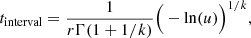
While with one-offs a 1D beam pattern suffices, a realistic simulation of the repeating population, as detected with large, asymmetric beams such as those used by CHIME, requires 2D beam patterns. To survey repeating populations, we used the formulas given in Gardenier et al. (2019) to simulate Gaussian and Airy beam patterns as 2D matrices, and we used a field-of-view (FoV) parameter to scale beam patterns relative to the survey. The Apertif and HTRU beam patterns available in frbpoppy can be scaled in a similar manner. The empirical mapping of the CHIME beam patterns is ongoing (see Berger et al. 2016), so to enable frbpoppy to conduct a chime-frb survey, we modelled our own CHIME-like beam pattern. To simulate this beam pattern, we convolved an Airy disk pattern orthogonal to a cosine function subtending an 80° ×180° area of the sky.
In Fig. 1, we show this CHIME-like beam pattern, with simulated observed tracks of several regular emitters at various declinations. The axes in Fig. 1, the N-S and E-W offset, refer to the relative offset along the N-S and E-W axes with respect to the center of the beam pattern. As expected, objects close to the North Pole are permanently visible. Objects at low declinations transit the beam. As all objects were emitting at the same cadence, the resulting spacing shows the transit speed.
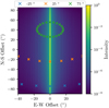 |
Fig. 1. Simulated beam pattern for the CHIME/FRB survey showing the transit of sources at various declinations as orthogonal offset along the north-south (N-S) and east-west (E-W) axes with respect to the centre of the beam pattern. All pointings are separated by an hour. |
Sets of survey parameters in frbpoppy allow it to model a range of current and future surveys (Gardenier et al. 2019). Additional parameters such as mount type and telescope location are required for the surveying of repeater populations. These are included in v2. Table 1 lists the main survey parameters adopted in the current paper.
Overview of the survey parameters adopted within this paper for a perfect and a chime-frb survey.
We next model different intrinsic source populations. Table 2 provides an overview of the required population parameters, and the relevant result figures per population. More information on these parameters is found in Gardenier et al. (2019).
Overview of parameters and values used to model intrinsic FRB source populations throughout this paper.
3. Results
3.1. Dispersion measure distributions
An important question in the FRB field is whether repeating and one-off FRB sources trace a single underlying population (e.g. Petroff et al. 2019; Cordes & Chatterjee 2019). One way to approach this question is to simulate a single repeating underlying FRB source population and compare the resultant observed repeating and one-off populations.
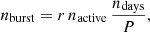
An initial hypothesis along these lines can be built as follows. We assume each source produces bursts following some luminosity distribution, where dim bursts outnumber bright bursts (for example: a power law with a negative index). We only probed the part of this distribution that is above a given sensitivity threshold. The further away, the higher and more limiting the corresponding luminosity threshold becomes; distant sources need to be far brighter to observe than sources close-by. Concerning repeaters, this effect is stronger than for one-offs. For them, at least two bursts drawn from this distribution must be seen above this threshold; whereas for one-offs, a single bright burst suffices. If all FRB sources have an equal chance of emitting from a range of luminosities, one would therefore expect the observed repeating population to drop off faster with distance than the observed one-off population. By using the dispersion measure (DM) as a proxy for distance, DM distributions can be used to probe this hypothesis.
We test this behaviour in Fig. 2, showing DM distributions for simulated intrinsic and simulated observed repeater populations. The observed population has been divided into ‘observed to be repeating’ sources (> 1 burst) and single-burst sources (1 burst). To simulate this population, we used parameters as given in the DM column of Table 2. To avoid conflating cosmological intricacies with repeater effects, we chose to simulate the cosmic population as a Euclidean population by limiting the maximum redshift zmax to 0.01. As the absolute scale of the resulting DM distributions is not of essence, we express this scale in Fig. 2 as a fraction of the total DM. For clarity, we modelled the extragalactic DM contribution solely with an intergalactic component, following Ioka (2003) in adopting DM = 1000z with DM in pc cm−3. Burst luminosities were drawn from a negative power law where N(L) ∝ Lli, with li being an index of −1.5 in the range of 1035 − 1040 ergs s−1, and they are drawn randomly per burst. The expression for the adopted power law can be converted into the form of dN(L)/dL ∝ L1 − γ when setting li = 1 − γ (cf. the definition in Lu et al. 2020). Changing these luminosity function parameters still results in similar behaviour to that shown in Fig. 2. To survey this cosmic population, we opted for a perfect survey (see Table 1). The perfect survey is practically noiseless; both the noise level and luminosity boundaries are therefore mere scaling factors rather than true expectations of parameter values. For this reason, we chose a very high signal-to-noise (S/N) limit of 106 to ensure only the high end of the flux distribution is probed.
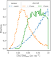 |
Fig. 2. Comparison between the simulated intrinsic and simulated observed dispersion measure distributions, expressed as a fraction of maximum DM. The normalised simulated intrinsic (cosmic) and observed populations are shown for repeaters in a Euclidean universe. Here the simulated observed population has been split into those seen as repeaters (> 1 burst) and those seen as one-offs (1 burst). |
Figure 2 shows that our simulations predict a clear distinction between the observed DM distribution of one-offs and repeaters, despite the fact that they emerge from the same cosmic population. These distributions follow our hypothesis that the observed repeater DM distribution would be expected to tail off faster with distance than that of the one-offs. Throughout the rest of this section, we refer to this expected difference as the DM discrepancy.
This emergence of a DM discrepancy relies chiefly on two assumptions. Firstly that all FRB sources repeat (see e.g. Spitler et al. 2016; Cordes & Wasserman 2016; Lyutikov et al. 2016; Katz 2017; Metzger et al. 2019), and secondly that the burst luminosity function is such that there are more low-energy bursts than energetic ones (see e.g. Macquart & Ekers 2018a; Luo et al. 2020; Fialkov et al. 2018). The results we obtain do not agree with early results from CHIME/FRB (Fonseca et al. 2020), which would seem to suggest that no difference is seen between the DM distribution of observed repeaters and one-offs.
Should a DM discrepancy remain unseen in future observations, it would lead to two possible main explanations and conclusions. Firstly, a negative power law may not necessarily be an accurate representation of the luminosity function of the intrinsic source population. Power laws are often used to approximate a wide range of physical processes, from the initial mass function (Salpeter 1955) to radiation from Shakura-Sunyaev thin accretion disks (Shakura & Sunyaev 1973). While there is an abundance of FRB progenitor theories (Platts et al. 2019), there is no conclusive theory on the expected emission process of an FRB. Recent detections of FRB-like bursts from a galactic magnetar (see e.g. Bochenek et al. 2020) may in time aid in constraining the emission mechanisms, but currently provide no prior expectation on the intrinsic luminosity function of the progenitor population. So which luminosity functions could reduce the expected DM discrepancy? As an example, flatter power laws could do this. The increase in the number of energetic repeat bursts leads to a higher chance of passing an S/N threshold. This follows recent research (e.g. Luo et al. 2020; Zhang et al. 2021) that advocates for flatter energy and luminosity indexes of, respectively, −0.7 and −0.8. However, simulations run with frbpoppy for this value still show a noticeable DM discrepancy. Schechter functions (Macquart & Ekers 2018a) do not necessarily solve this discrepancy problem either. The asymmetrical negative trend of these functions results in the same selection effects as in negative power laws. The DM discrepancy is avoided if the luminosity function gives repeating bursts an equal detection chance to the first detected burst. Such functions would include, for instance, standard candles, or distributions that are completely flat. Correlating observed burst luminosities with redshift estimates to FRB sources indicates that this is unlikely to be the case. Functions that are symmetric and completely visible at all distances would also explain these in principle, but they are not necessarily in agreement with observed number counts.
Secondly, the lack of a DM discrepancy could arise when the source populations of one-offs and repeaters are different in some respect. If one-off and repeating sources occupy slightly different parts of the parameter space, selection effects will weigh differently on both populations. This could bury the DM discrepancy. The culprit difference between one-offs and repeaters is not likely to be found in the number density distributions (which would follow from, for example, different progenitor populations). In observations, repeaters and one-offs seem to trace the same DM distribution, albeit with a different normalisation (Fonseca et al. 2020); such uniformity in the DM distributions while adopting different number densities would be contrived. The repeater population would also still be expected to show up in one-off distributions, albeit in a limited number, further complicating the situation. One might alternatively look towards the repetition rate as a source of difference, for instance by assuming one-off sources to intrinsically be one-offs. The impact on detection rates resulting from, for example, a difference in pulse-width distributions between one-offs and repeaters might also provide a way to hide the DM discrepancy, though it is unclear how.
For completeness, we note that the lack of an observed DM discrepancy could also be attributed to the survey. Should CHIME/FRB be sensitive to almost all repeaters, or simply observe for a long enough period of time, the DM discrepancy would disappear, with most repeaters being seen as repeaters. This is unlikely to be the case, however, given the sheer number of one-offs expected to have been detected by CHIME/FRB (McKinven 2020). To help constrain the origin of the lack of a DM discrepancy, we investigate similar selection effects in repeat bursts from repeating FRB sources in the next sub-section.
3.2. The repeat rate dependence on DM
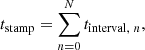
If the FRB luminosity function resembles a negative power law, as in the previous section, other similar observed effects may also be expected. We investigated the number of observed repeater bursts as a function of dispersion measure (Good 2020). In Fig. 3, the right axis marks the number of bursts per repeating source, as published in the CHIME/FRB repeaters database2 as of 2 September 2020. For a variety of luminosity functions, we compare these observations to the simulated observed average number of bursts per source, as marked on the left axis. Here, the negative power-law population is drawn from 1040 − 1045 ergs s−1 with an index of −1.5, the flat power law from the same range with an index of 0, and the standard candle population with bursts of 1042 ergs s−1. All other population parameters can be found in the rep-rate column of the population list (Table 2). Next, we simulated a perfect survey. An S/N limit of 4 × 10⁶ (non-physical, as in Sect. 3.1) provided the best visual fit in Fig. 3. Adopting a different S/N limit results in similar behaviour.
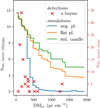 |
Fig. 3. Observed (crosses) and simulated (lines) number of observed bursts per repeater source, as a function of extragalactic dispersion measure. The red crosses show the observed burst rates from CHIME repeaters (scale on the right axis). The lines show the simulated average observed burst rates (scale on the left axis) for various luminosity functions along the same extragalactic dispersion measure axis. |
In this plot, we are interested in the detection-rate difference at low and high DM values. We adopted two y-axes in this figure for two reasons: firstly due to the limited number of CHIME/FRB repeaters, which would lead to poorly sampled bins; and, secondly, to allow for a relative scaling. In our simulations, we only aim to display the selection effects emerging from these luminosity functions, we have not yet aimed to reproduce the exact burst rates. Nonetheless, the behaviour of the simulated observations as shown in Fig. 3 still seem to suggest that selection effects due to a negative power-law luminosity function better describe the observed fast drop-off of repeater burst rates with DM than a flat luminosity function.
A drop-off in repeater burst rates can be expected for the same reasons as the DM discrepancy presented in Fig. 2: as the distance to a source increases, the chances of a burst falling above an S/N threshold decrease. We therefore expect to see more bursts for close repeaters than for distant ones, as is noted in the CHIME/FRB repeater data by Good (2020). While in a Euclidean universe the average number of observed bursts over the DM or redshift would be constant due to the time dilation, more distant sources have more bursts redshifted out of the observing time frame. This leads to the trends seen, for example, with standard candles or a flat power law, in which the average number of observed bursts drops off with distance.
The requirement here for a negative power law is somewhat at odds with explanation 1 from the previous section, which required a flat or symmetrical luminosity function to remove the expected DM discrepancy. Given how the selection effects from a negative power law can describe the repeater population, and that previous studies argue for a negative asymmetrical luminosity function such as a Schechter function (Macquart & Ekers 2018a; Luo et al. 2020; Fialkov et al. 2018), we conclude it is likely that the FRB population can be described as a whole with a negative power law. This means that explanation 2 for the lack of DM discrepancy as more likely: one-offs and repeaters subtend different parts of the intrinsic parameter space.
It is tempting to look to the repetition rate as a potential difference in parameter space, making one-offs intrinsically one-offs, or decreasing their likelihood to repeat. Determining the repeater fraction over time can help in establishing the veracity of such a claim. We discuss this in the next sub-section.
3.3. Repeater fraction
The physical or environmental relationship between repeating FRB sources and seemingly one-off FRB sources is as of yet unexplained. One line of thought is that the ostensible observed dichotomy may emerge from a single progenitor population (e.g. Cordes & Wasserman 2016; Metzger et al. 2019; Connor et al. 2020). Recent hints that these populations may have differing properties are emerging, however; whether in pulse widths (Fonseca et al. 2020), host galaxy properties (Heintz et al. 2020), or in dynamic spectra (Kumar et al. 2020). frbpoppy can be used to probe the hypothesis of FRBs emerging from a single source population. If all FRB sources repeat on different timescales, what would the expected observed repeater fraction as a function of time be? Could it correspond to the observed detections?
We started by considering how the fraction of detected sources that repeat (hereafter the repeater fraction frep) changes over time, based on two assumptions. We assumed the entire intrinsic FRB repeater source population shares a single distribution of repeat rates, such as a Poisson distribution. We also assumed a perfect survey with an S/N cut-off to limit sampling to the high end of a flux distribution. Taking these assumptions into consideration together, we would expect the repeater fraction to asymptotically reach one. The longer an observation, the more sources are seen to repeat. With an infinite time period, one would have seen all sources repeat.
A second step can be to instead introduce an intrinsic population in which all sources repeat following a Poissonian distribution, but all with a different Poissonian rate. To simulate this behaviour, the Poissonian rate distribution could be drawn from a normal distribution in the log space. Here too frep would asymptote towards a ratio of one, as all sources are eventually revealed to be repeaters. Nonetheless, we expect a sharper rise and slower tail on the value frep over time compared to the single-rate scenario. This expectation arises from the wide range of Poisson rates: some will have a short, and others a long, repetition scale. A Weibull distribution would introduce similar behavior, albeit more extreme. There, the clustering allows for the quick detection of some repeaters. But seeing many others repeat takes far longer, which is due to the longer time intervals resulting from a Weibull distribution.
In an alternative scenario, the population consists of a mix of repeating and one-off sources. How would the repetition rate differ in this case? For the repeating sources, one could expect the same behaviour as before: an asymptote towards the total fraction of repeaters. However, as the repeater fraction reaches that asymptote, it becomes increasingly likely for new detections to be one-offs. With more and more one-offs rather than repeating sources being detected, the repeater fraction will even start to show a turnover and will eventually decrease.
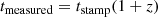
To simulate these cases, we generated a population using the parameters given in the rep-frac column of Table 2, and we surveyed this population using a perfect survey with an S/N limit of 104. We adopted population and survey parameters to reflect the most basic conditions under which these effects are still seen. The rate parameter used as population input is varied between a delta function at 0.1 day−1, a log-normal distribution with a rate of 0.1 day−1, a standard deviation of 2 day−1, and double delta function with peaks at 0 and 0.1 day−1, replicating a mix of one-offs and repeaters.
The results of these simulations can be seen in Fig. 4. Here, the left panel shows the distributions of the mean Poisson rate given as input, while the right panel shows the change in the repeater fraction over time. For illustrative purposes, we also show the results when a CHIME-like beam pattern was adopted for an otherwise perfect survey with an S/N cut-off at 1. These latter lines show the effect of beam patterns on the observed repeater fraction.
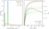 |
Fig. 4. Left: distributions of Poisson burst rate for various simulated intrinsic populations, including a single value (blue), a log-normal distribution (orange), and a mix of single values and one-offs (green). Right: repeater fraction frep, defined as the number of detected repeating sources over the total number of detected sources against time. The various line styles represent the detections from a perfect survey with an S/N cut-off with either a perfect beam pattern (solid), or a CHIME-like beam pattern (dotted). |
The first insight that the repeater fraction over time provides lies in the expected asymptote. This tells us the intrinsic repetition rate. If the observed repeater fraction tends towards an asymptote at unity, all FRB sources must repeat, albeit on a variety of timescales. The speed at which the asymptote is reached contains information on the intrinsic rate distribution. This is seen by comparing a population with a broad range of repetition rates to one with a narrow range. For the broad ranged population, fast repeaters are detected relatively quickly, leaving the slower repeaters to be detected over a longer timescale. The population with the same intrinsic Poissonian mean rate detects repeaters more uniformly. This effect is still observed after applying the CHIME-like beam pattern to the simulations. The dotted lines in Fig. 4 show this effect, with distinct differences between the various intrinsic rate distributions as input, but spread out over a longer timescale. This spreading is why the repeater fraction of the mixed input distribution does not display a downturn when adopting a CHIME-like beam pattern: that turnover occurs beyond the timescale of this graph. Measuring the repeater fraction over time, and by extension the intrinsic rate distribution from which it emerges, could help constrain possible rotational or orbital parameters of the repeating FRB population. This could help rule out some of the many possible progenitor theories (Platts et al. 2019).
The second insight comes from the value of the asymptote. The repeater fraction shows a sustained downturn over time, as seen, for instance, in the mixed population in Fig. 4. This indicates that one part of the FRB source population has been completely detected. That is evidence for a binarity in the repeating rates of the source population. This method would not provide any conclusive proof of the potential ‘one-off nature’ of one-offs, but it could constrain the population to a maximum observed time frame.
Determining this trend of the repeater fraction over time observationally will, as always, be more challenging than our perfect survey trends in Fig. 4. As seen when adopting a CHIME-like beam pattern as seen in Fig. 4, selection effects muddy the trend. Again, understanding the beam pattern of a survey to a high degree, by accurately mapping its intensity as function of position on sky, helps to recover a closer-to-intrinsic repeater fraction. Before an asymptote or downturn is actually reached, a fit to the observed repeater fraction might already be constraining enough to determine the values of these thresholds. This would additionally have the advantage of limiting the required observing time. While the repeater fraction is expected to initially show a rather jagged profile due to the limited number of repeaters versus one-offs, this effect should diminish over time as more repeaters are detected.
A number of repeaters follow Weibull distributions (Oppermann et al. 2018; Oostrum et al. 2020). We investigated how such distributions might affect the repeater fraction over time. Our simulations showed little difference compared to Poissonian rates. Some repeaters show rapidly clustered bursts and are quickly detected as repeaters, rapidly increasing the repeater fraction. The wait times for sources in the long tail of the Weibull distribution, however, severely decrease the rate at which the asymptote is reached.
Recent results show some repeaters have period windows of burst activity (Chime/FRB Collaboration 2020). If all repeaters display such cyclic behaviour, the repeater fraction trends would be noisier but still display the predicted trend.
The results we present here are in line with those from Ai et al. (2021), who conducted similar work investigating a repeater fraction over time. Their simulations show a reduced complexity, which is advantageous in computational time, but they lack the full range of selection effects present in frbpoppy. Given the strength of the selection effects in Fig. 4 (cf. Fig. 5), an accurate modelling of these selection effects is crucial to understanding the underlying source population.
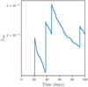 |
Fig. 5. Repeater fraction frep, is the number of sources observed to be repeating over the total number of observed sources, plotted over time for a full chime-frb simulation. |
3.4. Modelling CHIME/FRB detections
To infer the FRB progenitor population from the detected sources, we require the survey selection effects to be understood. CHIME/FRB has detected significantly more FRBs than any other survey to date (Fonseca et al. 2020). Modelling it and its selection effects is therefore crucial for the inclusion of this dataset, the largest one available, in population synthesis with frbpoppy. Incorporating the CHIME/FRB detections allows insights in both the one-off population model and the newly implemented repeater simulations.
As a basis for simulating an intrinsic repeating source population, we adopted the population parameters that replicate both HTRU and ASKAP-FLY one-off FRB detections (see Gardenier et al. 2019). These, along with newly adopted parameters, can be found in the complex column of Table 2. A number of parameters were changed with respect to the HTRU and ASKAP-FLY modelling. We chose, for instance, to limit the intrinsic population to a maximum redshift zmax of 1, a limit imposed by our compute resources. As most FRBs have low excess DM (Petroff et al. 2016), suggesting low redshifts, we chose our maximum redshift as a balance between simulation size and FRB detection volume. The adopted lower limit of the emission frequency was also increased by a single order of magnitude, to more fully sample the parameter space when adopting a negative spectral index. We simulate each FRB source to repeat with varying luminosities and pulse widths, a choice not available when modelling one-offs. We added the modelling of the intrinsic-burst time stamps. Here we adopted a log-normal distribution with a mean of nine bursts per day and a standard deviation of one burst per day. This distribution specifically refers to the intrinsic rate distribution rather than any observed rate distributions. To determine an optimum value for the number of sources ngen, the number of days ndays, and the mean rate for the log-normal time-stamp distribution, we ran a limited Monte Carlo simulation. The chosen values reflect the run that best replicated the expected CHIME/FRB detection fraction of ∼2.5 repeating and ∼200 one-off sources per 100 days. This corresponds to the expected CHIME/FRB detection rate of approximately two one-off sources per day (Chawla et al. 2017), while nine repeaters were detected over a little more than a year (Fonseca et al. 2020). To best direct our computational resources, we only simulated FRB sources in the sky area visible to our simulated CHIME telescope, representing 67.4% of the celestial sphere.
The next step is the simulation of CHIME/FRB detections. To that end, we adopted the complex survey parameters denoted in the chime-frb column of Table 1, together with the CHIME-like beam pattern described in Sect. 2.3.
3.4.1. Repeater fraction
Investigating if repeating and one-off FRB sources emerge from a single progenitor population is interesting for two reasons. First, the physics governing the burst generation, and second, the formation and evolution of the emitting sources. If there is only one source population, its radiation mechanism would need to be capable of producing both seemingly one-off bursts and repeating bursts. Next, both one-off and repeater detections, rates, and hosts could be used to determine the progenitor population. The question that we therefore seek to answer is: can an FRB population consisting entirely of repeaters explain the observed repeater versus one-off detection rates?
In Fig. 4, we showed the expected repeater fraction over time for various repeater distributions. The curves are smooth due to the high number of detections in the perfect survey: over 104 sources in 100 days. In Fig. 5, we replicate this plot, but for a full CHIME/FRB simulation over 100 days using a complex cosmic population and a chime-frb survey. A key difference between the chime-frb repeater fraction and the perfect survey plotted in Fig. 4 is the clear sawtooth effect, which arises from the limited number of repeaters detected by the simulated chime-frb over this timescale. After 100 days, 192 one-offs and 4
 repeaters were detected, close to the expected CHIME/FRB detection rate of 200 one-offs and two repeaters (Chawla et al. 2017; Fonseca et al. 2020). The errors on the simulated values represent the corresponding 1σ Poissonian intervals.
Our complex model is thus able to replicate the observed detection rates of both repeaters and one-offs, using an intrinsic source population consisting solely of repeaters. Modelling the repeater fraction over time is, however, merely one aspect of the observed FRB population available for analysis. Parameter distributions provide an alternative method by which the intrinsic FRB population can be probed.
3.4.2. DM and S/N distributions
Does the complex model also reproduce the observed distributions of FRB parameters? These distributions can give a handle on the progenitor population, provided the selection effects are well understood. Beyond replicating the detection rates as described above, we chose to investigate two aspects of the CHIME/FRB population: the DM and S/N distributions. The DM distribution as a proxy for a distance provides a way to roughly probe the observed number density of the FRB population. Our choice of S/N over similar parameters such as fluence, was made on the basis that it has the clearest meaning. It convolves all observatory-based selection effects, and hence provides the cleanest comparison between survey populations (James et al. 2019).
In Fig. 6, we show the repeater and one-off, DM, and S/N distributions, for real-observed and simulated-observed detections. All distributions weren normalised to their maximum values to allow the relative shapes of the distributions to be compared. For the repeaters, we plot the average DM value and the S/N of the first detected burst per source. We only used the first burst to avoid a bias arising from a single source saturating distributions with a high number of bursts. A Kolmogorov-Smirnov (KS) test was used to compare each set of distributions, of which the result is given in the top right of each panel. The real observed distributions were obtained from frbcat and the CHIME/FRB repeater database as of 2 September 2020. The simulated observed distributions use the complex model. Figure 6 shows a run from the small Monte Carlo simulation (Sect. 3.4) with the high KS test output. The p values are all above 0.05. Given the limited number of trials in the simulation, these p values indicate that the observations and simulations are consistent with being drawn from the same distribution. While these results are clearly based on very small numbers, they do indicate that the complex model can explain the observed CHIME/FRB populations to a reasonable degree.
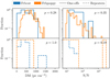 |
Fig. 6. Left column: real (blue) and simulated (orange) observed CHIME/FRB dispersion measure (DM) distributions for seemingly one-off sources (solid) and observed repeating sources (dashed). Right column: same groups, but showing the observed S/N distributions instead. In both cases, distributions were normalised to their maximum value to allow for comparison. Each panel shows the p-values from a KS-test conducted between both shown distributions. |
The simulated and real observed DM distributions for both one-off and repeating FRB sources are seen in the left column of Fig. 6. Although the limited number of detected repeaters necessarily makes comparisons challenging, the KS tests for these parameters indicate an encouraging match between observations and simulations for our complex model. In our simulations, the one-off and repeater populations span similar parts of the DM space, perhaps contrarily to expectations on the basis of Fig. 2. The reason is that the complex model underlying these simulated populations uses a flat luminosity index, which was shown to be able to replicated observed HTRU and ASKAP-FLY one-off detections, while the results given in Fig. 2 explored the impact of a negative index. The lack of a DM discrepancy corresponds to that seen in the CHIME/FRB data, in which both one-offs and repeaters are observed to follow the same distribution (Fonseca et al. 2020).
The S/N distributions for the simulated and observed repeater and one-off populations can be found in the right column of Fig. 6. The simulations also fit these distributions. The slopes for the one-off distributions are similar. There is a noticeable difference at low S/Ns, where frbpoppy expects more low-S/N events than observed. We conclude that CHIME becomes incomplete below S/N ≃ 15. Indeed, only comparing detections above an S/N limit of 15 gives a much improved fit, with a p-value of 0.98 for the one-offs. Potential explanations for the incompleteness are that the CHIME beam pattern is less sensitive than our simulated CHIME-like beam pattern, or that, for example, the RFI mitigation techniques adopted by CHIME/FRB block real low-S/N events (CHIME/FRB Collaboration 2018). For one-offs, it can be especially challenging to determine if a candidate is real, and lower S/N detections might therefore be disregarded out of caution. In repeaters, however, the same low-S/N candidate would be marked as real if prior bursts were detected at the same DM and location. For this reason, it can be important to compare possible selection effects in the detection pipeline of various surveys with, for instance, the benchmarking test set up for FRB detection pipelines (Connor 2020), similarly to prior work with pulsar pipelines (Lazarus et al. 2015). The simulated repeater distributions show a similar difference, with repeaters showing up at high S/Ns.
The first reason for taking caution in interpreting these fits is the low number of repeaters (just four) over this timescale; the second is the short simulation span of 100 days, while the real CHIME/FRB observations span a multiple of such a timescale. The single high-S/N event showing up in the simulated repeater distribution (Fig. 6) is curious, and on the basis of prior simulations, we believe it could be indicative of a slope more in line with that of the one-offs. This is in contrast with the observed CHIME distributions, where repeaters seem to show a steeper S/N distribution than one-offs. Including more newly published CHIME detections will help the investigation of this observed discrepancy and determining its origin.
An interesting statistical distinction between repeaters and one-off events is emerging in the CHIME data set. One-off FRBs appear to have narrower pulse widths than sources that have been detected twice or more (Fonseca et al. 2020). This effect may be due to an intrinsic difference between repeaters and non-repeaters, or due to an observational bias, as suggested by Connor et al. (2020). The effect does not appear in frbpoppy. This is unsurprising, because we did not model the FRB population as two separate source classes with different average widths, nor did we include beaming effects.
The simulations of the detection rates seen in Fig. 5 and the DM and S/N distributions seen in Fig. 6 match the observed CHIME/FRB population. As these complex population parameters also resulted in good fits to the observed one-off populations by HTRU and ASKAP (see Gardenier et al. 2019), they provide a solid basis from which the intrinsic FRB parameter space can further be explored. These fits additionally provide a good indication that a purely repeating population could describe the observed FRB populations. If so, observations focussing on one-off theories such as double neutron-star mergers (Totani 2013), double white-dwarf mergers (Kashiyama et al. 2013), or similar cataclysmic models could be dropped in favour of following expected observational signatures from repeating models such as from young magnetars (Metzger et al. 2019), flares from magnetar wind nebulae (Beloborodov 2017), or other models (see Platts et al. 2019).
The additional exploration of parameter spaces with frbpoppy is part of a subsequent investigation (Gardenier 2021). Further interpretation of the resulting population parameters will be carried out when CHIME FRBs are published.
3.5. Opportunities, uses, and further work
Our results demonstrate the value of FRB population synthesis, also for repeating sources. frbpoppy is open source by nature to encourage such use of FRB population synthesis. It can power research avenues ranging from simulations of the effect of different input distributions, to comparative studies of detections across various surveys. One clear result often cropping up in our simulations is the importance of the beam pattern. Shifting from extensive observations of single sources to probing the full FRB population will require team-derived and published beam patterns. Beam-pattern mapping has mostly been a focus of the imaging domain, yet understanding the effects of beam pattern on FRB detections will allow for much better probing of the intrinsic parameter space of the FRB source population. This would help in collating observations from multiple surveys to form a single, coherent picture of the FRB population.
4. Conclusions
We aimed to investigate whether one-offs and repeaters can emerge from the same intrinsic source population, and if selection effects explain the observed differences. We thus implemented repeating FRB sources in frbpoppy, an open source FRB population synthesis package in Python. We conclude the following:
-
Our simulations can reproduce current multi-survey observational data by synthesising a population solely including repeating FRBs, provided they have a wide distribution of repetition rates.
-
The luminosity function of FRBs can significantly impact the observed DM distribution of repeaters versus one-off detections (i.e. apparent non-repeaters). Should the DM distributions of repeaters and one-offs remain in agreement, as suggested by CHIME data, and evidence continue to point towards an intrinsic luminosity function described by a negative power law with more dim bursts than energetic ones, it could potentially suggest the presence of an intrinsic difference between repeating and one-off sources.
-
Within the observed repeater population, frequent repeaters tend to be closer and have smaller DMs. This effect was noticed in CHIME data by Good (2020), and we use frbpoppy to explain the inverse relationship between DM and repetition rate. The relationship is a consequence of point 2, and it indicates that the luminosity function of repeating FRBs is given by a negative power law with more dim bursts than energetic ones.
-
Fast radio burst surveys can use the observed repeater fraction over time to determine whether there is any binarity in the intrinsic repetition rate of the FRB source population. frbpoppy is the ideal tool for such an exercise because it can account for instrumental selection effects that are difficult to model analytically.
Overall, we thus find that the observed FRB sky can be explained by a single population of repeating FRBs that is uniform in its major characteristics, but where the repeat rate correlates with other, more minor, behavioural or physical traits.
To retrieve CHIME/FRB data, we made use of the pip-installable frbcat python package (Gardenier 2020), which is able to retrieve data from FRBCAT, the CHIME/FRB Repeater Database, and the Transient Name Server (TNS).
Acknowledgments
We thank the participants of FRB2020 for the fascinating conference, and especially Deborah Good for the illuminating discussion. The research leading to these results has received funding from the European Research Council under the European Union’s Seventh Framework Programme (FP/2007-2013)/ERC Grant Agreement n. 617199 (‘ALERT’); from Vici research programme ‘ARGO’ with project number 639.043.815, financed by the Netherlands Organisation for Scientific Research (NWO); and from the Netherlands Research School for Astronomy (NOVA4-ARTS). EP further acknowledges funding from an NWO Veni Fellowship. We acknowledge use of the CHIME/FRB Public Database, provided at https://www.chime-frb.ca/ by the CHIME/FRB Collaboration. We additionally acknowledge the use of the FRB catalogue ‘frbcat’ (Petroff et al. 2016), available at www.frbcat.org, and the use of NASA’s Astrophysics Data System Bibliographic Services. This research has made use of python3 (Van Rossum & Drake 2009) with numpy (van der Walt et al. 2011), scipy (Oliphant 2007), astropy (Astropy Collaboration 2018), pandas (McKinney et al. 2010), matplotlib (Hunter 2007), bokeh (Bokeh Development Team 2018), requests (Chandra & Varanasi 2015), sqlalchemy (Bayer et al. 2012), tqdm (da Costa-Luis et al. 2020), joblib (Joblib Development Team 2020), frbpoppy (Gardenier et al. 2019) and frbcat (Gardenier 2020).
References
- Ai, S., Gao, H., & Zhang, B. 2021, ApJ, 906, L5 [Google Scholar]
- Astropy Collaboration (Price-Whelan, A. M., et al.) 2018, AJ, 156, 123 [Google Scholar]
- Bayer, M. 2012, in The Architecture of Open Source Applications Volume II: Structure, Scale, and a Few More Fearless Hacks, eds. G. Wilson& A. Brown [Google Scholar]
- Beloborodov, A. M. 2017, ApJ, 843, L26 [Google Scholar]
- Berger, P., Newburgh, L. B., Amiri, M., et al. 2016, in Ground-based and Airborne Telescopes VI, SPIE Conf. Ser., 9906, 99060D [Google Scholar]
- Bochenek, C. D., Ravi, V., Belov, K. V., et al. 2020, Nature, 587, 59 [Google Scholar]
- Bokeh Development Team 2018, Bokeh: Python Library for Interactive Visualization http://www.bokeh.pydata.org [Google Scholar]
- Caleb, M., Stappers, B. W., Rajwade, K., & Flynn, C. 2019, MNRAS, 484, 5500 [Google Scholar]
- Chandra, R. V., & Varanasi, B. S. 2015, Python Requests Essentials (Packt Publishing Ltd) [Google Scholar]
- Chawla, P., Kaspi, V. M., Josephy, A., et al. 2017, ApJ, 844, 140 [Google Scholar]
- CHIME/FRB Collaboration (Amiri, M., et al.) 2018, ApJ, 863, 48 [Google Scholar]
- CHIME/FRB Collaboration (Amiri, M., et al.) 2019, Nature, 566, 235 [Google Scholar]
- Chime/FRB Collaboration (Amiri, M., et al.) 2020, Nature, 582, 351 [Google Scholar]
- Connor, L. 2020 Fast Radio Burst Detection: A benchmark comparing software packages that detect fast radio bursts (FRBs) https://www.eyrabenchmark.net/benchmark/4fcec5b8-40ad-4ca7-a663-c4f96c52bd19 [Google Scholar]
- Connor, L., Miller, M. C., & Gardenier, D. W. 2020, MNRAS, 497, 3076 [Google Scholar]
- Cordes, J. M., & Wasserman, I. 2016, MNRAS, 457, 232 [Google Scholar]
- Cordes, J. M., & Chatterjee, S. 2019, ARA&A, 57, 417 [Google Scholar]
- Cruces, M., Spitler, L. G., Scholz, P., et al. 2020, MNRAS, 500, 448 [Google Scholar]
- da Costa-Luis, C., Larroque, S. K., Altendorf, K., et al. 2020, https://doi.org/10.5281/zenodo.4054194 [Google Scholar]
- Fialkov, A., Loeb, A., & Lorimer, D. R. 2018, ApJ, 863, 132 [Google Scholar]
- Fonseca, E., Andersen, B. C., Bhardwaj, M., et al. 2020, ApJ, 891, L6 [Google Scholar]
- Gardenier, D. W. 2020, frbcat: Fast Radio Burst CATalog Querying Package Astrophys. Source Code Libr., [record ascl:2011.011] [Google Scholar]
- Gardenier, D. W. 2021, PhD Thesis, University of Amsterdam [Google Scholar]
- Gardenier, D. W., van Leeuwen, J., Connor, L., & Petroff, E. 2019, A&A, 632, A125 [Google Scholar]
- Ghirlanda, G., Ghisellini, G., Salvaterra, R., et al. 2013, MNRAS, 428, 1410 [Google Scholar]
- Good, D. 2020, Fast Radio Burst 2020 Thailand Meeting http://frb2020.phys.wvu.edu/ [Google Scholar]
- Gourdji, K., Michilli, D., Spitler, L., et al. 2019, ApJ, 877, L19 [Google Scholar]
- Gu, W.-M., Dong, Y.-Z., Liu, T., Ma, R., & Wang, J. 2016, ApJ, 823, L28 [Google Scholar]
- Heintz, K. E., Prochaska, J. X., Simha, S., et al. 2020, ApJ, 903, 152 [Google Scholar]
- Hewish, A., Bell, S. J., Pilkington, J. D. H., Scott, P. F., & Collins, R. A. 1968, Nature, 217, 709 [Google Scholar]
- Hunter, J. D. 2007, Comput. Sci. Eng., 9, 90 [NASA ADS] [CrossRef] [Google Scholar]
- Ioka, K. 2003, ApJ, 598, L79 [Google Scholar]
- Izzard, R. G., & Halabi, G. M. 2018, ArXiv e-prints [arXiv:1808.06883] [Google Scholar]
- James, C. W., Ekers, R. D., Macquart, J. P., Bannister, K. W., & Shannon, R. M. 2019, MNRAS, 483, 1342 [Google Scholar]
- James, C. W., Osłowski, S., Flynn, C., et al. 2020, ApJ, 895, L22 [Google Scholar]
- Joblib Development Team 2020, Joblib: Running Python Functions as Pipeline Jobs [Google Scholar]
- Johnston, S., Bailes, M., Bartel, N., et al. 2007, PASA, 24, 174 [Google Scholar]
- Kashiyama, K., Ioka, K., & Mészáros, P. 2013, ApJ, 776, L39 [Google Scholar]
- Katz, J. I. 2017, MNRAS, 467, L96 [Google Scholar]
- Kumar, P., Shannon, R. M., Flynn, C., et al. 2020, MNRAS, 500, 2525 [Google Scholar]
- Lazarus, P., Brazier, A., Hessels, J. W. T., et al. 2015, ApJ, 812, 81 [Google Scholar]
- Lu, W., Piro, A. L., & Waxman, E. 2020, MNRAS, 498, 1973 [Google Scholar]
- Lundgren, S. C., Cordes, J. M., Ulmer, M., et al. 1995, ApJ, 453, 433 [Google Scholar]
- Luo, R., Men, Y., Lee, K., et al. 2020, MNRAS, 494, 665 [Google Scholar]
- Lyutikov, M., & Popov, S. 2020, ArXiv e-prints [arXiv:2005.05093] [Google Scholar]
- Lyutikov, M., Burzawa, L., & Popov, S. B. 2016, MNRAS, 462, 941 [Google Scholar]
- Maan, Y., & van Leeuwen, J. 2017, 2017 XXXIInd General Assembly and Scientific Symposium of the International Union of Radio Science (URSI GASS), 2 [Google Scholar]
- Macquart, J.-P., & Johnston, S. 2015, MNRAS, 451, 3278 [Google Scholar]
- Macquart, J. P., & Ekers, R. D. 2018a, MNRAS, 474, 1900 [Google Scholar]
- Macquart, J. P., & Ekers, R. 2018b, MNRAS, 480, 4211 [Google Scholar]
- Macquart, J.-P., Bailes, M., Bhat, N. D. R., et al. 2010, PASA, 27, 272 [Google Scholar]
- Macquart, J. P., Shannon, R. M., Bannister, K. W., et al. 2019, ApJ, 872, L19 [Google Scholar]
- Masui, K., Lin, H.-H., Sievers, J., et al. 2015, Nature, 528, 523 [Google Scholar]
- McKinney, W., et al. 2010, Proceedings of the 9th Python in Science Conference, 445, 51 Austin, TX [Google Scholar]
- McKinven, R. 2020, Fast Radio Burst 2020 Thailand Meeting, http://frb2020.phys.wvu.edu/ [Google Scholar]
- Metzger, B. D., Margalit, B., & Sironi, L. 2019, MNRAS, 485, 4091 [Google Scholar]
- Oliphant, T. E. 2007, Comput. Sci. Eng., 9, 10 [Google Scholar]
- Oostrum, L. C., Maan, Y., van Leeuwen, J., et al. 2020, A&A, 635, A61 [CrossRef] [EDP Sciences] [Google Scholar]
- Oppermann, N., Yu, H.-R., & Pen, U.-L. 2018, MNRAS, 475, 5109 [Google Scholar]
- Petroff, E., & Chatterjee, S. 2020 Fast Radio Burst Community Newsletter - Issue 11 (Cornell University Library) [Google Scholar]
- Petroff, E., Johnston, S., Keane, E. F., et al. 2015, MNRAS, 454, 457 [Google Scholar]
- Petroff, E., Barr, E. D., Jameson, A., et al. 2016, PASA, 33, e045 [Google Scholar]
- Petroff, E., Hessels, J. W. T., & Lorimer, D. R. 2019, A&ARv, 27, 4 [Google Scholar]
- Platts, E., Weltman, A., Walters, A., et al. 2019, Phys. Rep., 821, 1 [Google Scholar]
- Rajwade, K. M., Mickaliger, M. B., Stappers, B. W., et al. 2020, MNRAS, 495, 3551 [Google Scholar]
- Salpeter, E. E. 1955, ApJ, 121, 161 [Google Scholar]
- Shakura, N. I., & Sunyaev, R. A. 1973, A&A, 500, 33 [NASA ADS] [Google Scholar]
- Shannon, R. M., Macquart, J. P., Bannister, K. W., et al. 2018, Nature, 562, 386 [Google Scholar]
- Snyder, J. P. 1987, Map projections-A Working Manual (US Government Printing Office), 1395 [Google Scholar]
- Spitler, L. G., Scholz, P., Hessels, J. W. T., et al. 2016, Nature, 531, 202 [Google Scholar]
- Taylor, J. H., & Manchester, R. N. 1977, ApJ, 215, 885 [Google Scholar]
- Thornton, D., Stappers, B., Bailes, M., et al. 2013, Science, 341, 53 [Google Scholar]
- Totani, T. 2013, PASJ, 65, L12 [Google Scholar]
- van der Walt, S., Colbert, S. C., & Varoquaux, G. 2011, Comput. Sci. Eng., 13, 22 [Google Scholar]
- Van Rossum, G., & Drake, F. L. 2009, Python 3 Reference Manual (Scotts Valley, CA: CreateSpace) [Google Scholar]
- Zhang, R. C., Zhang, B., Li, Y., & Lorimer, D. R. 2021, MNRAS, 501, 157 [Google Scholar]
Appendix A: Tracking celestial objects
Determining the path of a celestial object through a beam pattern is a non-trivial challenge. To simulate the surveying of a repeating FRB population, frbpoppy incorporates functions to calculate the position of objects within a beam pattern. In frbpoppy, we approached this challenge by transforming source coordinates to the coordinate system relative to the beam pattern. These transformations differ depending on the type of telescope mount involved.
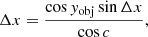
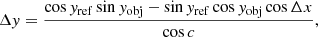
In frbpoppy, we chose to model beam patterns in 2D matrices, yet we generated source coordinates in a (3D) equatorial coordinate system. Here, we used 3D to refer to a coordinate system such as right ascension and declination, which by definition describe angles on a unit sphere in 3D space. Determining the position of a celestial object in a beam pattern therefore requires mapping from 3D to 2D. Adopting a gnomonic projection for this transformation allows a beam pattern to be expressed in units of angular offset (degrees) relative to a central pointing. We followed Snyder (1987) in expressing the gnomonic projection as follows:
 (A.1)
(A.1)
 (A.2)
(A.2)
 (A.3)
(A.3)
 (A.4)
(A.4)
 (A.5)
(A.5)
with Δx/Δy being the orthogonal offset in 2D, xref/yref the 3D reference (or pointing) angular coordinates, and xobj/yobj the 3D object’s angular coordinates. We note that these equations are only valid when cos c > = 0, and they are undefined when cosc < 0. This limit represents pointings on the sky beyond the observable horizon of a telescope located on a sphere.
For observatories with equatorial mounts, celestial objects remain in a constant position with respect to the beam pattern of a single pointing of a single-dish telescope. As such, the right ascension α and declination δ can be adopted directly as, respectively, x and y in Eqs. (A.1)–(A.5). This avoids any additional transformations of the reference and object coordinates.
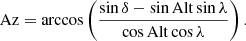
Azimuthally mounted telescopes, however, do not retain a constant angle with respect to the North Pole, leading objects to wander through a beam pattern over the course of a single pointing. In frbpoppy, we model detections by such telescopes by shifting source pointings from an equatorial to an azimuthal coordinate system. We assume a survey to start at a random point of time in this century, and for both the relative and object coordinates, we calculate the local hour angle:
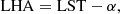 (A.6)
(A.6)
with the local hour angle LHA, local sidereal time LST, and right ascension α. Taking this together with the declination δ and the latitude of a telescope λ allows the altitude Alt and azimuth Az to be calculated:
 (A.7)
(A.7)
 (A.8)
(A.8)
For LHA > 0, an E-W correction has to be applied in the form of Az = 360 − Az. The resulting azimuth and altitude of both the object and the reference point can subsequently be used as x and y in Eqs. (A.1)–(A.5).
Transit observatories can be modelled in a similar fashion to azimuthally mounted telescopes. By fixing the reference coordinate to the zenith, source coordinates can be transformed into the azimuthal coordinate system using Eqs. (A.6)–(A.8) before making use of Eqs. (A.1)–(A.5).
All Tables
Overview of the survey parameters adopted within this paper for a perfect and a chime-frb survey.
Overview of parameters and values used to model intrinsic FRB source populations throughout this paper.
All Figures
|
Fig. 1. Simulated beam pattern for the CHIME/FRB survey showing the transit of sources at various declinations as orthogonal offset along the north-south (N-S) and east-west (E-W) axes with respect to the centre of the beam pattern. All pointings are separated by an hour. |
| In the text | |
|
Fig. 2. Comparison between the simulated intrinsic and simulated observed dispersion measure distributions, expressed as a fraction of maximum DM. The normalised simulated intrinsic (cosmic) and observed populations are shown for repeaters in a Euclidean universe. Here the simulated observed population has been split into those seen as repeaters (> 1 burst) and those seen as one-offs (1 burst). |
| In the text | |
|
Fig. 3. Observed (crosses) and simulated (lines) number of observed bursts per repeater source, as a function of extragalactic dispersion measure. The red crosses show the observed burst rates from CHIME repeaters (scale on the right axis). The lines show the simulated average observed burst rates (scale on the left axis) for various luminosity functions along the same extragalactic dispersion measure axis. |
| In the text | |
|
Fig. 4. Left: distributions of Poisson burst rate for various simulated intrinsic populations, including a single value (blue), a log-normal distribution (orange), and a mix of single values and one-offs (green). Right: repeater fraction frep, defined as the number of detected repeating sources over the total number of detected sources against time. The various line styles represent the detections from a perfect survey with an S/N cut-off with either a perfect beam pattern (solid), or a CHIME-like beam pattern (dotted). |
| In the text | |
|
Fig. 5. Repeater fraction frep, is the number of sources observed to be repeating over the total number of observed sources, plotted over time for a full chime-frb simulation. |
| In the text | |
|
Fig. 6. Left column: real (blue) and simulated (orange) observed CHIME/FRB dispersion measure (DM) distributions for seemingly one-off sources (solid) and observed repeating sources (dashed). Right column: same groups, but showing the observed S/N distributions instead. In both cases, distributions were normalised to their maximum value to allow for comparison. Each panel shows the p-values from a KS-test conducted between both shown distributions. |
| In the text | |
Current usage metrics show cumulative count of Article Views (full-text article views including HTML views, PDF and ePub downloads, according to the available data) and Abstracts Views on Vision4Press platform.
Data correspond to usage on the plateform after 2015. The current usage metrics is available 48-96 hours after online publication and is updated daily on week days.
Initial download of the metrics may take a while.