| Issue |
A&A
Volume 646, February 2021
|
|
|---|---|---|
| Article Number | A153 | |
| Number of page(s) | 10 | |
| Section | Extragalactic astronomy | |
| DOI | https://doi.org/10.1051/0004-6361/202039576 | |
| Published online | 19 February 2021 | |
A possible sub-kiloparsec dual AGN buried behind the galaxy curtain
1
INAF-Osservatorio Astronomico di Brera, Via Brera 28, 20121 Milano, Italy
e-mail: This email address is being protected from spambots. You need JavaScript enabled to view it.
2
Institute of Theoretical Astrophysics, University of Oslo, PO Box 1029, Blindern 0315, Oslo, Norway
3
Dipartimento di Fisica e Astronomia, Alma Mater Studiorum, Università degli Studi di Bologna, Via Gobetti 93/2, 40129 Bologna, Italy
4
INAF-Osservatorio di Astrofisica e Scienza delle Spazio di Bologna, OAS, Via Gobetti 93/3, 40129 Bologna, Italy
5
Dipartimento di Fisica “G. Occhialini”, Universià di Milano-Bicocca, Piazza della Scienza 3, 20126 Milano, Italy
6
INFN-Sezione di Milano-Bicocca, Piazza della Scienza 3, 20126 Milano, Italy
7
INAF-Osservatorio Astronomico di Roma, Via Frascati 33, 00078 Roma, Italy
8
Dipartimento di Matematica e Fisica, Università degli Studi Roma Tre, Via della Vasca Navale 84, 00146 Roma, Italy
9
XMM-Newton Science Operations Centre, ESAC/ESA, PO Box 78, 28691 Villanueva de la Cañada, Madrid, Spain
Received:
2
October
2020
Accepted:
16
December
2020
Abstract
Although thousands of galaxy mergers are known, only a handful of sub-kiloparsec-scale supermassive black hole (SMBH) pairs have been confirmed so far, leaving a huge gap between the observed and predicted numbers of such objects. In this work, we present a detailed analysis of the Sloan Digital Sky Survey optical spectrum and of near-infrared (NIR) diffraction limited imaging of SDSS J1431+4358. This object is a local radio-quiet type 2 active galactic nucleus (AGN) previously selected as a double AGN candidate on the basis of the double-peaked [OIII] emission line. The NIR adaptive optics-assisted observations were obtained at the Large Binocular Telescope with the LUCI+FLAO camera. We found that most of the prominent optical emission lines are characterized by a double-peaked profile, mainly produced by AGN photoionization. Our spectroscopical analysis disfavors the hypothesis that the double-peaked emission lines in the source are the signatures of outflow kinematics, leaving open the possibility that we are detecting either the rotation of a single narrow-line region or the presence of two SMBHs orbiting around a common central potential. The latter scenario is further supported by the high-spatial resolution NIR imaging: after subtracting the dominant contribution of the stellar bulge component in the host galaxy, we detect two faint nuclear sources at r < 0.5 kpc projected separation. Interestingly, the two sources have a position angle consistent with that defined by the two regions where the [OIII] double peaks most likely originate. Aside from the discovery of a promising sub-kiloparsec scale dual AGN, our analysis shows the importance of an appropriate host galaxy subtraction in order to achieve a reliable estimate of the incidence of dual AGNs at small projected separations.
Key words: galaxies: individual: SDSS J143132.84+435807.20 / galaxies: active / galaxies: interactions / quasars: emission lines / infrared: galaxies / black hole physics
© ESO 2021
1. Introduction
In the last few decades, the presence of supermassive black holes (SMBHs) at the centers of massive galaxies and the existence of correlations between their masses and their host galaxy bulges were observationally uncovered by different authors (e.g., Soltan 1982; Haehnelt & Rees 1993; Kormendy & Richstone 1995; Faber 1999; O’Dowd et al. 2002; Häring & Rix 2004; Ferrarese & Ford 2005; Kormendy & Ho 2013; Savorgnan et al. 2016). As a result of gas accretion onto the SMBH, a large amount of energy can be released, leading to the ignition of an active galactic nucleus (AGN; Soltan 1982; Hopkins et al. 2007; Ueda et al. 2014). Galaxy interactions are one of the main processes that can drive gas inflows toward the nuclear region, thus triggering the AGN activity (Hernquist 1989; Barnes & Hernquist 1991; Mihos & Hernquist 1996; Barnes 2002; Springel 2005; Li et al. 2007; Hopkins & Hernquist 2009; Capelo & Dotti 2017; Blumenthal & Barnes 2018). Therefore, if SMBHs are ubiquitously present in the center of galaxies, the formation of dual AGNs (kiloparsec separation) is expected in a large fraction of merging and merged galaxies. Following the Λ cold dark matter (ΛCDM) cosmological paradigm predictions, in which galaxies grow hierarchically through (minor and major) mergers, dual AGNs should be located in a large number of sources.
Many of the systematic searches conducted so far are based on the quest for double-peaked narrow optical emission lines originating from two distinct narrow-line regions (NLRs). These studies yield a detection rate of a few percent of confirmed dual AGNs (see, e.g., Shen et al. 2011; Fu et al. 2012; Liu et al. 2011). The incidence of confirmed dual AGNs in merging system samples (Koss et al. 2012; Teng et al. 2012; Mezcua et al. 2014) or among the candidates selected by radio surveys (Burke-Spolaor 2011; Fu et al. 2015a,b; Burke-Spolaor et al. 2018) is slightly higher, but still below 10%, hence very low with respect to the expectations based on the merger rate of galaxies (e.g., Springel et al. 2005; Hopkins et al. 2005; Van Wassenhove et al. 2012; Capelo et al. 2017). However, it is important to note that all these observational studies suffer from biases that could significantly reduce the detection rate of dual AGNs. Some of these biases (e.g., the wavelength used, the incompleteness of the samples, and the difficulty in resolving the pairs at small projected separations) are widely discussed in Solanes et al. (2019) and some of these biases are also addressed in this work.
In principle, if we could assess from observations the exact incidence of dual AGNs, we would constrain galaxy evolutionary models and study the final stages of the merging process (Van Wassenhove et al. 2012; Blecha et al. 2013; Colpi 2014). Moreover, during the formation of dual systems, significant negative or positive feedback can be produced (see, e.g., Koss et al. 2012; Blecha et al. 2013; Mezcua et al. 2014; Rubinur et al. 2020), affecting both the interstellar and circum-galactic media. Furthermore, dual AGNs are the direct precursors of binary SMBHs (sub-parsec and parsec-scale separations), which are amongst the loudest emitters of gravitational waves in the frequency ranges detectable by pulsar time arrays (PTAs; Verbiest et al. 2016) and by the future space-based gravitational wave Laser Interferometer Space Antenna (LISA; Amaro-Seoane et al. 2017). For these compact systems direct imaging is beyond the capability (i.e., angular resolution) of any current instrument, except for high-resolution interferometric observations of radio emitting sources (see, e.g., Rodriguez et al. 2006; Kharb et al. 2017; Deane et al. 2014, but see also Wrobel et al. 2014). Regarding the binary SMBHs with projected separation below the very long baseline interferometry (VLBI) resolution limits, an exemplary case is the blazar OJ 287. For this object a strong indication of the SMBH binary nature comes from a complex modeling of optical and radio variability (Valtonen et al. 2008; Valtonen & Pihajoki 2013; Britzen et al. 2018; Dey et al. 2019). A still scarce list of few additional promising binary SMBH candidates is available in the literature (see, e.g., Boroson & Lauer 2009; Tsalmantza et al. 2011; Eracleous et al. 2012; Decarli et al. 2013; Ju et al. 2013; Shen et al. 2013; Liu et al. 2014; Graham et al. 2015; Runnoe et al. 2017; Wang et al. 2017; Severgnini et al. 2018; Serafinelli et al. 2020).
Although observationally more accessible, even dual AGNs at kiloparsec and sub-kiloparsec separations require stringent angular resolution to be directly imaged, and the current instrumental limitations make their detection particularly challenging. Among the few tens of SMBHs at < 10 kpc separation confirmed so far, only a few (∼10) are unambiguous sub-kiloparsec pairs of SMBHs (see Das et al. 2018; Rubinur et al. 2018; De Rosa et al. 2019, and references therein for exhaustive lists of confirmed dual AGNs). At present, about 30% of the confirmed dual AGNs have been selected from double-peaked narrow optical emission line sources (Fu et al. 2011; McGurk et al. 2015). In this respect, the catalogs of Wang et al. (2009), Smith et al. (2010), Liu et al. (2010), and Ge et al. (2012) provide more than a thousand of unique AGNs with a double-peaked [OIII]λ5008 Å line identified using the Sloan Digital Sky Survey Data Release 7 (SDSS-DR7; Abazajian et al. 2009). We note that, for low-redshift sources (i.e., z ≤ 0.15), the 3″ diameter of the SDSS data fiber ensures that the double-peaked emission lines come from a physical region smaller than 10 kpc. Unfortunately, the SDSS fiber does not allow us to discern whether the double-peaked emission lines are due to dual nuclei or to kinematical effects occurring in the surrounding of a single AGN, that is, jet-cloud interactions or outflows (Heckman et al. 1984; Whittle et al. 2005; Rosario et al. 2010; Gabányi et al. 2017), a rotating, disk-like NLR (Xu & Komossa 2009; Müller-Sánchez et al. 2011), or the combination of a blobby NLR and extinction effects (Crenshaw et al. 2010). Therefore, follow-up observations, including high-spatial resolution imaging combined with spatially resolved spectroscopy, have been used by different authors to further investigate the kinematical origin of double-peaked emission lines (see, e.g., Fu et al. 2011, 2012; McGurk et al. 2015; Tingay & Wayth 2011; Comerford et al. 2012; Müller-Sánchez et al. 2015).
In principle, high-spatial resolution (sub-arcsec) observations allow us to identify dual AGNs down to sub-kiloparsec scale. Nevertheless, a strong limitation is that strict observability constraints are often needed to achieve the required sub-arcsec imaging quality, which limits the number of dual AGN candidates that could be investigated in detail so far. This is particularly true for radio-quiet objects, which represent the majority of the AGN population. Optical and near-infrared (NIR) imaging performed with adaptive optics (AO) systems requires both optimal seeing conditions and the presence of at least one bright point-like source within much less than one arc minute by the target. X-ray observations could reach the sub-arcsec spatial resolution with the Chandra sub-pixel imaging technique (see, e.g., Fabbiano et al. 2018). However, in this case, a rather large amount of net counts (at least 500−1000) are required, limiting the studies to very few bright nearby dual AGN candidates.
By combining the results of the four spectroscopic samples quoted above (Wang et al. 2009; Smith et al. 2010; Liu et al. 2010; Ge et al. 2012), there are ∼930 AGNs at z ≤ 0.15 with a double-peaked [OIII]λ5008 Å line and only 5% of these objects have been followed-up with sub-arcsec spatial resolution imaging in the optical and/or NIR bands (i.e., Fu et al. 2012; McGurk et al. 2015). For only a small fraction (∼17%), a companion within 3″ (less than 10 kpc of projected separation at z ≤ 0.15) has been directly discerned in the sub-arcsec resolution imaging and thus further investigated through spatially resolved spectroscopy as possible dual AGNs. As we discuss in this paper, the fraction of dual AGNs on kiloparsec and sub-kiloparsec scales could be higher than that inferred by searching for a companion directly visible on sub-arcsec imaging. Even high-resolution imaging may miss the presence of multiple nuclear components if their emission is dimmed by dust and gas and/or blended with a dominant diffuse stellar bulge component from the host galaxy.
In this paper we present the results obtained on a radio-quiet1 dual AGN candidate: SDSS J143132.84+435807.20 (type 2, z = 0.09604, hereafter SDSS J1431+4358), which belongs to the samples of Wang et al. (2009) and Ge et al. (2012). The NIR follow-up was performed with the LUCI camera, in diffraction-limited mode, at the Large Binocular Telescope (LBT). As we show in this work, to maximize the possibility of identifying multiple nuclei, the dominant stellar contribution should be adequately taken into account and subtracted.
This galaxy shows a clear double-peaked [OIII] emission line in the SDSS-DR7 optical spectrum (Wang et al. 2009; Ge et al. 2012), which prompted a follow up by Nevin et al. (2016) with spatially resolved long-slit spectroscopy. In Sect. 2, we summarize the previous results, while in Sect. 3 we present our analysis of the SDSS-DR152 spectrum, along with the observations and the analysis we performed on the LBT and on the Swift-X-ray Telescope (Swift-XRT) data of SDSS J1431+4358. The results are presented in Sect. 4. In Sect. 5, we combine the spectroscopical information with the NIR results in light of the most plausible physical scenarios for SDSS J1431+4358. Section 6 presents our conclusions.
Throughout the paper we assume a flat ΛCDM cosmology with H0 = 69.6 km s−1 Mpc−1, Ωλ = 0.7 and ΩM = 0.3. All the magnitudes are in the Vega system. Errors are given at 68% confidence level.
2. SDSS J1431+4358
SDSS J1431+4358 is a local (z = 0.09604) bulge-dominated galaxy (see also Sect. 3.2) which, from a visual inspection, appears isolated and undisturbed (see also Ge et al. 2012). It belongs to a sample of 87 SDSS-DR7 type 2 AGNs with double-peaked [OIII] profiles selected and analyzed by Wang et al. (2009). In that work, the [OIII] line was fit with a blueshifted (Δλb=−2.89 ± 0.33 Å) and a redshifted (Δλr = 3.23 ± 0.35 Å) component, neither of which is at the systemic velocity of the host galaxy. The corresponding fluxes of the blueshifted and redshifted components as estimated by Wang et al. (2009) are as follows: F[OIII]blue = (66 ± 9) × 10−17 erg cm−2 s−1 and F[OIII]red = (60 ± 9) × 10−17 erg cm−2 s−1. The source is also included in the double-peaked emission-line galaxy sample selected by Ge et al. (2012). These authors investigated the nature of each peak component through the Baldwin-Phillips-Terlevich diagram (BPT, Baldwin et al. 1981) and inferred that both the blue and red components for SDSS J1431+4358 are produced by AGN photoionization.
SDSS J1431+4358 was further observed by Nevin et al. (2016) with the Apache Point Observatory Dual Imaging Spectrograph (0.42″ pix−1 in the blue channel, 0.4″ pix−1 in the red channel). The authors investigated the origin of double-peaked narrow lines for a sample of double-peaked type 2 AGNs at z < 0.1 through spatially resolved long-slit spectroscopy. Observations at two position angles were obtained for each source to constrain the orientation of the NLR. As quoted by Nevin et al. (2016), while they were unable to directly identify dual AGNs with long-slit data alone, they defined a classification method to distinguish NLR kinematic classification as rotational or outflow-dominated. As for SDSS J1431+4358, the two positional angles used during the observations were orthogonal (PAobs1 = 87 deg and PAobs2 = 177 deg) and one of these is coincident with the photometric major axis of the host galaxy, as derived from the SDSS r-band photometry (PAgal = 87 deg). Following Nevin et al. (2016), the inferred NLR position angle is PA[OIII] = 59 deg. By analyzing the double-peaked profiles at each spatial position, the authors found the possible presence of a broad [OIII] emission line component (σ > 500 km s−1) in the spectrum collected along the positional angle of PAobs1 = 87 deg. Although the very large uncertainties associated with the velocity dispersion value (σ = 578 ± 283 km s−1) make the detection of a broad [OIII] component only tentative, Nevin et al. (2016) classified the NLR kinematics as possibly outflow-dominated (see also Müller-Sánchez et al. 2011).
As discussed in the next sections, although the spectral analysis does not rule out the presence of an ionized outflow component, we find that this mechanism can hardly be the main origin of the double-peaked emission lines observed in the optical spectrum of SDSS J1431+4358.
3. Observations and data analysis
3.1. The SDSS-DR15 optical spectrum
We analyzed the publicly available SDSS-DR15 optical spectrum of SDSS J1431+4358 (see Fig. 1) focusing on the presence and the properties of double-peaked emission line profiles. We first fitted the host galaxy spectral stellar continuum using the penalized PiXel-Fitting method (pPXF; Cappellari & Emsellem 2004; Cappellari 2017) with the Medium resolution INT Library of Empirical Spectra (MILES) single stellar population (SSP) models (Vazdekis et al. 2010). We did not allow pPXF to fit the nebular emission lines as well, since we do this fit in a second stage using our own procedures. The obscuration of the active nucleus allowed us to determine the redshift of the host galaxy (z = 0.09597 ± (6 × 10⁻⁵)) through the stellar absorption lines. In Fig. 1 the best-fitting MILES model is overlaid on the rest-frame SDSS-DR15 spectrum. The residuals obtained by the subtraction of the stellar component from the observed spectrum are also shown. In the following, we present the analysis performed on the residual spectrum. We verified that our results do not depend (within the 1σ uncertainties) on the subtracted stellar continuum by running the spectral fitting subtraction several times and with different templates.
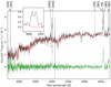 |
Fig. 1. SDSS J143132.84+435807.20 rest-frame SDSS-DR15 spectrum (black line). The strongest emission lines are labeled and an inset of the spectrum covering the [OIII]λ5008 Å (rest–frame vacuum wavelengths) emission line is shown. The red curve indicates the best-fitting MILES model resulting from the pPXF spectral fitting (see Sect. 3.1), while the green spectrum indicates the residual obtained after the subtraction of the stellar component from the observed spectrum. |
For the spectral modeling we used the Python package SHERPA3. To investigate the presence and the properties of the double-peaked profiles, we mainly focused on the [OIII]λ4960 Å, λ5008 Å, Hα + [NII]λ6550 Å, λ6585 Å, and [SII]λ6718 Å, λ6733 Å emission lines. For the remaining and less prominent emission lines visible in the spectrum (i.e., [OII] and [OI]; see Fig. 1) the spectral fitting analysis does not allow us to reach reliable conclusions. In particular, the [OII] emission line is a doublet (λ3727 Å and λ3730 Å); these emission lines are too close in wavelengths and would require a higher spectral quality (both in term of spectral resolution and signal-to-noise ratio) to detect and properly model any double peak. Regarding the [OI] emission line, it could be equally well fitted by two narrow Gaussian components or by a single one plus broad wings. A broad component is often observed for the [OI], which is generally interpreted as evidence that the emitting clouds are optically thick to the ionizing radiation (Osterbrock 1991). In the observed spectrum the Hβ line is only seen in absorption. However, once we subtract the dominant galaxy contribution, as shown in Fig. 1, a weak narrow emission component emerges. Owing to the low signal-to-noise ratio (S/N ∼ 3 at the emission line peak), it is not possible to statistically distinguish if the Hβ emission line profile is better reproduced by a single or double emission line components. We performed the spectral fitting of the residual spectrum in the rest-frame 4820−4900 Å spectral range by assuming both a single and double Gaussian components. In the first case, we found that the Hβ emission line can be well reproduced by a narrow (full width at half maximum, FWHM ∼ 390 km s−1, FHβ ∼ 19 × 10−17 erg cm−2 s−1) Gaussian component at the systemic velocity of the host galaxy. The best-fit parameters found by assuming two Gaussian components are reported in Table 1. In this case, since the widths of the emission components result unconstrained, we assumed that they are on the same order, in units of km s−1, of those estimated for the strongest narrow emission lines present in the spectrum (see below).
Best-fit values of the most prominent emission line components in the SDSS-DR15 spectrum of SDSS J1431+4358 (see Fig. 1).
[OIII]λ4960 Å, λ5008 Å emission lines – As shown in the zoomed part of the spectrum in Fig. 1, the [OIII]λ5008 Å emission line clearly presents a double-peaked profile. We considered the residual spectrum (see Fig. 1) in the rest-frame 4930−5040 Å spectral region. This covers both the [OIII]λ4960 Å and the [OIII]λ5008 Å emission lines and excludes spectral zones where absorption lines are present. We used a combination of a power-law continuum plus two Gaussian components for each of the [OIII] emission lines. The emission line centroids and their relative intensities were set to be all independent. We allowed their widths to be free to vary, but we kept the width of the blue (red) [OIII]λ4960 Å emission line component tied to the blue (red) [OIII]λ5008 Å line component. The results of the fit are shown in Fig. 2, panels a and b, where the only significant residuals (∼3σ) are visible around 5018−5020 Å. The addition of a narrow (FWHM ∼ 250 km s−1) Gaussian emission line component at 5020 Å statistically improves the fit at more than 99.99% confidence level. The wavelength of this narrow line coincides with the rest-frame wavelength of the strongest Fe II emission line group emitting between 4930 and 5050 Å (a6S–z6Po transition, multiplet 42), typically observed in the type 1 and narrow line Seyfert 1 spectra (see e.g., Véron-Cetty et al. 2004). We checked that the other emission lines associated with the same iron transition (i.e., around at 4924 Å and around at 5169 Å) are also present in the SDSS J1431+4358 spectrum. With the exception of the iron excess, only very low statistical significance (∼2σ) residuals are present in the residual shown in panel b and no further components are requested by the fit. In spite of this, following the Nevin et al. (2016) results on the possible presence of an outflowing material, we also included two additional broad Gaussian emission line components (see panels c and d of Fig. 2). The first component is around the 4940−4955 Å excess and a second is around the 4990−5000 Å excess (both denoted as “wing?” in Fig. 2). For both of these, we found similar FWHM (∼500 km s−1) and similar offset central wavelength (∼−700 km s−1) with respect to the [OIII]λ4960 Å and the [OIII]λ5008 Å emission lines, respectively.
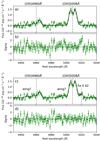 |
Fig. 2. Residual spectrum of SDSS J1431+4358 (green symbols in this figure and in Fig. 1) around the [OIII]λ4960 Å, λ5008 Å emission line region. The spectrum is shown in the rest-frame vacuum wavelengths. The gray dashed vertical lines indicate the position of the emission line at the systemic velocity of the host galaxy as derived by the stellar absorption lines. Panel a: the black solid line represents the model obtained by the combination of a power-law continuum plus two Gaussian emission line components for each of the [OIII] lines. Panel b: relevant residuals, shown in terms of sigmas. Panel c: the black solid line indicates the model obtained by adding a Gaussian component at 5020 Å (denoted as Fe II 42) and two broad Gaussian components (denoted as “wing?”, see Sect. 3.1) to the basic model shown in panel a. Panel d: relevant residuals, shown in terms of sigmas. |
Best-fit values relevant to the [OIII] narrow emission lines are reported in Table 1; we note that they do not depend on the adopted model (with or without broad wings). Our results on the [OIII]λ5008 Å lines are in agreement, within the uncertainties, with those obtained by Wang et al. (2009) in terms of peak offsets and line flux values.
Hα + [NII]λ6550 Å, λ6585 Å emission lines – As in the case of the [OIII]λ5008 Å, also the Hα emission line shows a clear double-peaked profile (see Fig. 3). To include both the Hα and the [NII] lines in our anlaysis, we fitted the residual spectrum of SDSS J1431+4358 between 6525 Å and 6615 Å. The Hα profile requires two Gaussian components, both of which are characterized by a FWHM on the same order as the [OIII]λ5008 Å widths. Conversely, the [NII] emission lines can be fitted well by a single broader Gaussian having FWHM similar to the combination of the two (blue and red) [OIII]λ5008 Å components (i.e., ∼650−700 km s−1). However, we note that the worse resolving power at higher wavelengths (from ∼2.5−3800 Å to ∼3.6−9000 Å), combined with the larger critical electron density for de-excitation of the [NII] transition with respect to the [OIII], can broaden the line profile slightly (Osterbrock 1991). This in turns implies that, with the quality of the current spectra, an intrinsically double-peaked profile for the [NII] emission line would appear as a single broad line. To test if the apparent broadening could be due to the presence of double-peaked lines, we replaced each of these lines with two emission lines. We thus make the approximation that the two [NII] emission lines (at 6550 Å and 6585 Å) are both double-peaked as well. We then assumed that their widths are on the same order, in units of km s−1, of those estimated for the other narrow emission lines (i.e., [OIII] and Hα). In particular, we tied the [NII] widths to the [OIII] values. In this case, two Gaussian components are clearly requested to reproduce each of the [NII] emission lines. The fitting results are showed in Fig. 3 while the best-fit parameters are reported in Table 1.
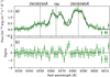 |
Fig. 3. Residual spectrum of SDSS J1431+4358 (green symbols in this figure and in Fig. 1) around the Hα + [NII]λ6550 Å, λ6585 Å emission line region. The spectrum is shown in the rest-frame vacuum wavelengths. The gray dashed vertical lines mark the position of the emission line at the systemic velocity of the host galaxy. Panel a: the black solid line is the model obtained by the combination of a power-law continuum plus two Gaussian emission line components for both the Hα and for each of the [NII] emission lines. Panel b: relevant residuals, shown in terms of sigmas. |
[SII]λ6718 Å, λ6733 Å emission lines – The spectral region around the [SII] emission lines is shown in Fig. 4. As for the [NII] emission lines, we assumed the emission line widths of the [SII] components to be equal to those of the [OIII] emission lines, in units of km s−1. Although with larger uncertainties, we found that also in this case, each of the [SII] emission lines can be well reproduced by the combination of two Gaussian components (see Fig. 4 and Table 1).
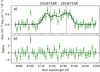 |
Fig. 4. Residual spectrum of SDSS J1431+4358 (green symbols in this figure and in Fig. 1) around the [SII]λ6718 Å, λ6733 Å emission line region. The spectrum is shown in the rest-frame vacuum wavelengths. The gray dashed vertical lines indicate the position of the emission line at the systemic velocity of the host galaxy. Panel a: the black solid line represents the model obtained by the combination of a power-law continuum, plus two Gaussian emission line components for each of the [SII] emission lines. Panel b: relevant residuals, shown in terms of sigmas. |
3.2. Observations by LBT
We observed the dual AGN candidate, SDSS J1431+4358 (KS ∼ 13.8 mag4) with the LBT-LUCI2 camera (one of the two LBT Utility Cameras in the Infrared; Seifert et al. 2003) with the First Light Adaptive Optics system (FLAO; Esposito et al. 2012) in diffraction limited mode. The observations were performed on 9 May 2018 (Program ID: LBT-2018A-C1349-12, P.I. Severgnini) in the K band using the N30-camera (pixel scale of 0.015 arcsec pix−1) for a total exposure time of 1800 s and on-source exposure time of 1200 s. The observations were conducted under a natural seeing condition of 0.7″ (FWHM), which allowed us to reach an image quality of 0.15″ (FWHM).
The LUCI data reduction pipeline developed at INAF – Osservatorio Astronomico di Roma5 was used to perform the basic data reduction that includes dark subtraction, bad pixel masking, cosmic ray removal, flat fielding, and sky subtraction. Astrometric solutions for individual frames were obtained, and the single frames were then recombined using a weighted co-addition to obtain the final stacked image normalized to 1 s of exposure. In Fig. 5 (left panel), we show a zoom on the 5″ × 5″ reduced K-band image. The target is clearly resolved (Fig. 5, right panel) and bulge dominated. As expected on the basis of the optical spectrum (see Fig. 1) and on the basis of the R − K color (∼2.3 mag), typical of local normal galaxies (e.g., Mannucci et al. 2001; Chang et al. 2006), the host galaxy emission not only dominates the optical bands but also the NIR band. This implies that, if a nuclear component is present, regardless of whether it is a single or a double component, its infrared emission is completely diluted by the host galaxy emission and therefore, it cannot be directly detected without a proper bulge component subtraction from the NIR image.
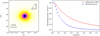 |
Fig. 5. Left panel: zoomed (5″ × 5″) K-band image of SDSS J1431+4358 taken with LBT+LUCI+FLAO in diffraction-limited mode. Right panel: normalized radial profiles in the K-band, measured within circular annuli centered on the target (SDSS J1431+4358, red points) and on the point-like source (blue points) used for the PSF reconstruction at about 5.5″ from the target (see Sect. 3.2). |
Photometric fitting residuals: GALFIT
Since the double nuclei could be hidden by the galaxy continuum emission, we then proceeded to fit the galaxy profile and subtracted it from the data. We used the 2D fitting algorithm GALFIT (Peng et al. 2002, 2010) and adopted for the galaxy the 1D Sérsic profile (Sérsic 1963)
![Mathematical equation: $$ \begin{aligned} I(r)=I_{\rm e} \exp \left[-b_{n}\left(\left(\frac{r}{r_{\rm e}}\right)^{\frac{1}{n}} - 1\right)\right], \end{aligned} $$](/articles/aa/full_html/2021/02/aa39576-20/aa39576-20-eq1.gif) (1)
(1)
where Ie is the pixel surface brightness at radius re and the shape of the profile is determined by the Sérsic index n. This function allows us to model an exponential disk (n = 1) or a classical bulge component, which is usually characterized by n > 2, and in particular the de Vacouleurs profile (de Vaucouleurs 1948) with n = 4.
To fit the galaxy profile of SDSS J1431+4358, we convolved a 2D Sérsic model with the point spread function (PSF). For the PSF, we used the true image of a high S/N point-like source in the LUCI field of view, located at 5.5″ from the target galaxy (the 1D profile is shown in the right panel of Fig. 5, blue points). In the fitting procedure we also used a flat background sky and allowed the centroid (x, y), the Sérsic index n, the effective radius Re and the total magnitude to vary. The galaxy contribution is well reproduced (χ2/d.o.f. = 1.03) with a Sérsic index n = 4.8 ± 0.1 and an effective radius Re = (2.7 ± 0.1)″ = (4.8 ± 0.1) kpc.
In Fig. 6, we compare the radial profile measured from the K-band image, using circular annuli centered on the nuclear source (red points), and the predicted radial profile derived from the best-fitting Sérsic model (blue points). Within ∼0.2″ of radius, positive residuals with respect to the Sérsic model are present, possibly resulting from the AGN contribution. The residual image produced by GALFIT in the central 0.24″ × 0.24″ region is shown in Fig. 7 (left panel). The image reveals the presence of two possible distinct nuclear components at projected separation of ∼0.12″, as measured from the distance of the two brightest pixels. The northern and brighter component has a projected position almost spatially coincident with the host galaxy center. The measured positional angle is ≈50 deg, in agreement with the orientation measured for the NLR (Nevin et al. 2016, PA[OIII] ∼ 59 deg). The contour levels in Fig. 7 (left panel) show the pixels with a value from 2.5 to 4 times the standard deviation of the background.
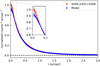 |
Fig. 6. Radial profiles, as measured within circular annulus on the K-band image and centered on the target (SDSS J1431+4358, red points), compared with the surface brightness from the best-fitting Sérsic model profile (blue points). Both profiles are normalized to the peak value of the source. |
In order to assess whether two point–like sources at such a small angular separation can be resolved by AO assisted LUCI observations, we performed some basic simulations with GALFIT. We modeled the two point-like sources by convolving two Gaussians, which have the minimum FWHM value allowed by GALFIT (FWHM = 1.5 × 10⁻³ arcsec), with the true PSF of the image (see above). We then added the true background rms derived by the real image. We produced several simulated images for different values of the relative intensity and separation between the two point-like sources. We verified that down to an angular separation of about 0.12″ the two simulated sources appear to be resolved. In particular, we found that the two observed NIR blobs can be reproduced well by two sources at ∼0.12−0.2″ apart (corresponding to ∼215−360 pc). The K-band magnitudes of the northern and southern simulated sources are ∼19 mag and ∼20 mag, respectively. Since these magnitudes were estimated by imposing that the emission peaks in the simulated images had the same value as the peaks in the real image, they strongly depend on the adopted background noise. Using different background rms image derived by different zones of the real image, we estimated that the uncertainties on the magnitudes are on the order of 1 mag. As an example of our simulations, in Fig. 7 (right panel) we show one of the simulated residual maps obtained by using two point-like sources with a relative distance of 0.12″ and with K-magnitudes equal to 19.5 mag and 20.3 mag.
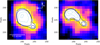 |
Fig. 7. Left panel: K-band residual image (0.24″ × 0.24″) centered on SDSS J1431+4358. The image was obtained by smoothing the real K-band residual image with a Gaussian filter (σ = 1 pixel = 0.015″; see Sect. 3.2). Contour plots are overlaid: the dark blue (light blue) lines indicate the pixels with a value of 2.5 and 2.7 (3 and 4) times the standard deviation of the background of the unsmoothed residual image. Right panel: simulated image, obtained by considering two point-like sources (relative distance of 0.12″ and with K-magnitudes equal to 19.5 mag and 20.3 mag), the true PSF image, and the background sky (see Sect. 3.2 for details). The image was obtained by smoothing the simulated image with a Gaussian filter (σ = 1 pixel = 0.015″). Contour plots are overlaid: The dark blue (light blue) lines indicate the pixels with a value of 2.5 and 2.7 (3 and 4) times the standard deviation of the background of the unsmoothed simulated image. |
3.3. Swift-XRT observation
As X-ray data were not available for SDSS J1431+4358, we recently were awarded an explorative observation with the Swift-XRT (Burrows et al. 2005). This observation was carried out through a Target of Opportunity (ToO) request (5 ks, Target ID: 13292, observation date: 2020 March 18). The 0.3−10 keV image was extracted using the online XRT data product generator6 (Evans et al. 2007, 2009). SDSS J1431+4358 was not detected down to a 3σ limiting flux of about 10−13 erg cm−2 s−1. We note that the source was not detected in the 0.3−4 keV and 4−10 keV images either.
4. Results
Our analysis of the SDSS spectrum (Sect. 3.1) confirms the type 2 spectroscopic classification of SDSS J1431+4358 (Wang et al. 2009; Ge et al. 2012). The lack of significant broad emission line components up to the Hα wavelengths suggests an intrinsic AV ≥ 3 mag (e.g., Gilli et al. 2001).
We found that both the [OIII]λ5008 Å and the Hα emission lines show a clear double-peaked profile, which is well fitted by two narrow Gaussian components. Once we constrain the FWHM of the other emission lines, which are present in the spectrum, to be on the same order of the width of the [OIII] lines, we also found that the [NII] and the [SII] emissions could be accounted for by two Gaussian emission line components. The shifts between the blue (red) peak and the systemic redshift are similar, within the uncertainties, for all the observed transitions across the full spectral range (see Table 1). In particular, for the [OIII]λ5008 Å and the Hα emission lines, for which the presence of double components are clearly evident, neither the blue nor the red peaks are consistent with the nominal systemic velocity of the host galaxy (derived independently from the stellar absorption lines). We found that the flux ratios between the blue and red peaks are on the order of one for most of the more prominent emission lines.
Regarding the Hβ transition, a weak narrow emission line is visible only in the residual spectrum, while in the observed spectrum the relevant stellar absorption component fully overwhelms it. Owing to the low S/N, the emission line profile can be fitted well by either a single (see Sect. 3.1) or double Gaussian components (see Table 1).
We then investigated the nature of the ionizing source producing the blue and red peak components through the BPT diagnostic diagram (see Fig. 8). From this figure we can see that both the blue and red peaks detected in the SDSS J1431+4358 spectrum occupy the AGN locus, where the gas is mainly photoionized by the AGN emission (see also Ge et al. 2012).
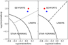 |
Fig. 8. BPT diagram of the blue (blue star symbol) and red (red star symbol) components detected in the optical spectrum of SDSS J1431+4358. The solid and dashed lines divide the regions mainly populated by star-forming galaxies and AGN from Kewley et al. (2001, 2006) and Kauffmann et al. (2003), respectively. The dotted and dot-dashed lines demarcate the Seyfert and LINER zones from Cid Fernandes et al. (2010) and Kewley et al. (2006), respectively. |
In agreement with the results found by Nevin et al. (2016), our analysis does not rule out the presence of an ionized outflow component; indeed, a faint [OIII] broader (FWHM ∼ 500 km s−1) blue wing is tentatively detected. However, this component cannot explain the double-peaked profile of the [OIII] line. This latter is reproduced well by two further narrow Gaussian components (blue- and redshifted, respectively) with similar peak intensities.
The K-band emission of SDSS J1431+4358, as well as the optical emission, is fully dominated by the host galaxy contribution. Thanks to the tight sub-arcsec sampling provided by the LBT-LUCI NIR camera in AO mode (0.015″ pix−1), we unveiled significant residuals in the nuclear zone (within 0.2 arcsec) with respect to the expectation for a single galaxy model. After subtracting the host galaxy contribution, two spatially distinct NIR components emerge at sub-kiloparsec separation. Intriguingly, the positional angle of the two NIR sources (PANIR ∼ 50 deg) is close, within a typical error of 15 deg, to that estimated for the two emitting NLR (PA[OIII] ∼ 59 deg; Nevin et al. 2016). However, the authors do not provide the physical projected offset of the two NLR centroids.
SDSS J1431+4358 was not detected in our Swift-XRT observation. The 3σ upper limit on the X-ray flux of about 10−13 erg cm−2 s−1 (see Sect. 3.3) could be an indication of the presence of high obscuration in the X-ray band as well. We calculated the most plausible unabsorbed X-flux from the [OIII] de-reddened luminosity (![Mathematical equation: $ L^{\mathrm{c}}_{\mathrm{[OIII]}} $](/articles/aa/full_html/2021/02/aa39576-20/aa39576-20-eq2.gif) ). We first applied the hydrogen Balmer decrement correction to the total luminosity7 of the [OIII]λ5008 Å emission line,
). We first applied the hydrogen Balmer decrement correction to the total luminosity7 of the [OIII]λ5008 Å emission line,
![Mathematical equation: $$ \begin{aligned} L^\mathrm{c}_{\rm [OIII]}=L_{\rm [OIII]}{\left[\frac{(\mathrm{H}\alpha /\mathrm{H}\beta )_{\rm obs}}{3.0}\right]}^{2.94} \end{aligned} $$](/articles/aa/full_html/2021/02/aa39576-20/aa39576-20-eq3.gif) (2)
(2)
where (Hα/Hβ)obs-pagination is the observed line ratio (Osterbrock & Ferland 2006). Then, by adopting the ![Mathematical equation: $ L_{\mathrm{X}}{-}L^{\mathrm{c}}_{\mathrm{[OIII]}} $](/articles/aa/full_html/2021/02/aa39576-20/aa39576-20-eq4.gif) relation reported by Lamastra et al. (2009) and Panessa et al. (2006), we predicted an unabsorbed 0.3−10 keV flux on the order of about 5 × 10⁻¹³ erg cm−2 s−1 and 10−12 erg cm−2 s−1, respectively (well above the derived upper limit). We then assumed that the intrinsic X-ray emission is a power law with the typical photon index of Γ = 1.8 and estimated the amount of absorption that could explain the nondetection in the XRT observation. We found that we need a column density of the absorbing gas in excess of 1022–1023 cm−2.
relation reported by Lamastra et al. (2009) and Panessa et al. (2006), we predicted an unabsorbed 0.3−10 keV flux on the order of about 5 × 10⁻¹³ erg cm−2 s−1 and 10−12 erg cm−2 s−1, respectively (well above the derived upper limit). We then assumed that the intrinsic X-ray emission is a power law with the typical photon index of Γ = 1.8 and estimated the amount of absorption that could explain the nondetection in the XRT observation. We found that we need a column density of the absorbing gas in excess of 1022–1023 cm−2.
5. Discussion
SDSS J1431+4358 was first selected as a type 2 dual AGN candidate by Wang et al. (2009) on the basis of the double-peaked profile of the [OIII]λ5008 Å emission line. The presence of narrow emission lines with double-peaked profiles was subsequently confirmed by Ge et al. (2012), who pointed out that both the blue- and the redshifted emission lines are produced by AGN photoionization. Our independent analysis corroborates these results.
Interestingly, the misalignment measured by Nevin et al. (2016) between the position of the NLR and the major axis of the host galaxy (PA[OIII] = 59 deg and PAgal = 87 deg) disfavors the possibility that double-peaked NLRs are tracing the gas kinematics of the host galaxy.
In these previous works (Wang et al. 2009; Ge et al. 2012; Nevin et al. 2016), the lack of a dual core detection in the SDSS images left equally open the hypotheses of a single SMBH or of double SMBHs. In the first case, the kinematical origin of the detected double-peaked profiles could be due to outflows or to rotational effects of a single NLR disk-like, while in the second case, they could trace the orbital motion of the two SMBHs around a common central potential.
The typical signature for outflowing and/or inflowing components in integrated galaxy spectra is the presence of fainter and blue and/or red broader emission lines superimposed on the narrow emission line centered at the systemic velocity (e.g., Harrison et al. 2014, 2016). The spectroscopical analysis presented in this work confirms the possible presence of an ionized outflow component, previously also detected by Nevin et al. (2016). However, we found that the same outflow mechanism can hardly explain the presence of two narrow emission lines (blue- and redshifted, respectively) with similar peak intensities (as in the case of SDSS J1431+4358, see Table 1). The receding sides of ionized outflows traced by optical nebular lines are usually undetected (or extremely faint) owing to extinction by dust in the center of the galaxy and in the outflow itself. So, in the case of SDSS J1431+4358, there are two possibilities. First, if we ascribe only the blue component to an outflow (in addition to the blueshifted wing at ∼−700 km s−1 tentatively detected in the [OIII] transitions and shown in Fig. 2), then it would mean that the red component of the line traces the systemic NLR emission, which would be redshifted by ∼210 km s−1 with respect to the host galaxy redshift determined via the stellar absorption. Second, if instead we ascribe both components to a symmetric red- plus blueshifted outflow, then it would mean that there is no dust obscuration since both components are detected at the same level, and that there is no NLR emission at the systemic velocity. Basically, it would imply that all of the nebular emission comes from an outflow. This would be very odd, and it is a situation that has not been observed even in the most powerful outflows observed so far; there is always a quiescent narrow line component. So the only viable interpretation is that neither of the two components traces an outflow.
According to Smith et al. (2012), a flux ratio on the order of one between the blue and red peaks could be considered as an indication for the presence of a single, rather than a double, ionizing source. However, we note that, while in the majority of the cases this could be true, it cannot be used to discard the presence of two distinct SMBHs in individual systems. The hydrodynamic simulations of galaxy mergers presented by Blecha et al. (2013) showed that in the presence of dual SMBHs, emission line profiles with almost even peaks may arise at one viewing angle at least. The same authors concluded that AGNs with uneven-peaked narrow emission line profiles have at most a modestly higher probability of containing two SMBHs than AGNs with an even-peaked profiles.
Because of the large amount of nuclear absorption affecting the AGN intrinsic emission (i.e., the power law plus the broad emission line components), the source appears as a bulge-dominated galaxy up to the NIR band. After subtracting the host galaxy contribution in the high-resolution NIR LBT image, we detect, for the first time, two compact components at a sub-kiloparsec projected separation in the SDSS J1431+4358 core. While the NIR imaging data alone do not allow us to discard the possibilities that the fainter NIR core can be associated with a smaller merging stellar bulge or to an outflow component, the close spatial alignment between the two NIR cores and the two regions where double-peaked AGN emission lines originate (Nevin et al. 2016) supports the presence of a dual AGN.
Under this hypothesis, the minimum estimated distance of the two SMBHs is about 215−360 pc (see Sect. 3.2). This implies that the two putative accretion disks (of typical radius less than 0.01 pc) should be undisturbed and could illuminate the surrounding gas forming two NLRs. Thus, the double-peaked profiles could trace the motions of two distinct or semi-detached NLRs orbiting around a common central potential.
An alternative scenario, in which double peaks are produced by two almost co-spatial and disturbed NLRs forming a single envelope rotating around the two SMBHs cannot be fully discarded, but it is less likely. In this case, the narrow emission line regions may be partially destroyed or deformed. A more complex emission line profiles would be expected with respect to the almost regular double profiles observed for SDSS J1431+4358 (see, e.g., Popović 2012).
A further possibility is that we are seeing the rotational effect associated only with the brightest and dominant of the two NLRs, that is, the NLR that is rotating around the most powerful of the two SMBHs (Popović 2012; Blecha et al. 2013).
Only future high-resolution and spatially resolved spectroscopical observations will provide a definitive answer on the nature of SDSS J1431+4358 and on the origin of its double-peaked emission lines. This will allow us to confirm or rule out the spatial coincidence of the double line emission components with the two NIR cores.
6. Summary and conclusions
We presented the spectral analysis of the archival SDSS-DR15 optical spectrum and the analysis of new LBT-LUCI NIR sub-arcsec observation for SDSS J1431+4358, a local radio-quiet type 2 AGN previously selected as double AGN candidate.
As for the optical spectrum, all the most prominent emission lines are characterized by a double-peaked profile. On the basis of the flux line ratios, we found that all the emission line components are mainly produced by AGN photoionization. Although the presence of outflowing ionized material cannot be disfavored, because a third blue and broad [OIII] emission line is tentatively detected, it can hardly be the cause of the two relatively narrow components of the double-peaked profiles. Rotational effects due to a single NLR associated with a single SMBH or due to the presence of two SMBHs are the most likely hypothesis for the double-peaked emission lines observed in our target.
The presence of a dual AGN is strengthened by the high-spatial resolution NIR imaging. In particular, the tight sub-arcsec sampling provided by the LUCI-AO camera allowed us to detect significant residuals in the central zone of the galaxy. Once we subtracted the host contribution, two faint central NIR sources emerged. Interestingly, the two central cores have a positional angle similar to the positional angle of the two emitting regions where the [OIII] double peaks most likely originate. The cause of the apparent faintness in the optical and in the NIR bands of the two putative nuclear sources could be explained with the presence of a large amount of intrinsic obscuration affecting the central region.
Although only high-resolution and spatially resolved spectroscopy will definitely set the spatial coincidence of the double NLR regions with the double NIR cores, the multiwavelengths results presented in this work favor the hypothesis of a double sub-kiloparsec scale SMBH. Up to now, dedicated spatially resolved spectroscopy aimed at confirming the presence of a double AGN were carried out only on candidates presenting two cores directly discerned in radio, optical or NIR high-resolution imaging (see, e.g., Fu et al. 2012; McGurk et al. 2015; Müller-Sánchez et al. 2015; Das et al. 2018, and references therein). Only a handful of dual AGNs with a separation smaller than about 0.5 kpc have been discovered so far. However, the pre-selection of interesting candidates was generally performed without subtracting the contribution of the host galaxy contribution. The analysis presented in this paper shows that the lack of an appropriate host galaxy subtraction could prevent us from unveiling the presence of two distinct cores located in a single merged galaxy. This clearly affects the estimates of their fraction among the AGN population. Thus, in addition to the discovery of a new promising sub-kiloparsec scale dual AGN, our analysis also suggests that the real fraction of dual AGNs among double-peaked emission line sources could be underestimated (Liu et al. 2010; Comerford et al. 2012; Fu et al. 2012; Müller-Sánchez et al. 2015; McGurk et al. 2015).
The source is undetected down to about 1 mJy (5σ) at 1.4 GHz in the VLA FIRST survey (Becker et al. 1995).
The SDSS-DR15 acronym means that the spectrum was downloaded by the Sloan Digital Sky Survey Data Release 15 website: http://skyserver.sdss.org/dr15/en/home.aspx
The KS magnitude was taken by the final release of the 2MASS extended objects, https://irsa.ipac.caltech.edu/cgi-bin/Gator/nph-dd
We considered as total line luminosity the sum of the luminosities of the blue and red components reported in Table 1.
Acknowledgments
We thank the anonymous referee for her/his valuable suggestions which improved the quality of the paper. We acknowledge the support from the LBT-Italian Coordination Facility for the execution of observations, data distribution and reduction. VB, RDC, RS, PS, and AZ acknowledge financial contribution from the agreements ASI-INAF n.2017-14-H.0 and n.I/037/12/0. This work is based on data supplied by the UK Swift Science Data Centre at the University of Leicester. The SDSS is managed by the Astrophysical Research Consortium for the Participating Institutions of the SDSS Collaboration (see http://www.sdss.org/collaboration/citing-sdss/).
References
- Abazajian, K. N., Adelman-McCarthy, J. K., Agüeros, M. A., et al. 2009, ApJS, 182, 543 [Google Scholar]
- Amaro-Seoane, P., Audley, H., Babak, S., et al. 2017, ArXiv e-prints [arXiv:1702.00786] [Google Scholar]
- Baldwin, J. A., Phillips, M. M., & Terlevich, R. 1981, PASP, 93, 5 [NASA ADS] [CrossRef] [EDP Sciences] [Google Scholar]
- Barnes, J. E. 2002, MNRAS, 333, 481 [Google Scholar]
- Barnes, J. E., & Hernquist, L. E. 1991, ApJ, 370, L65 [Google Scholar]
- Becker, R. H., White, R. L., & Helfand, D. J. 1995, ApJ, 450, 559 [NASA ADS] [CrossRef] [Google Scholar]
- Blecha, L., Loeb, A., & Narayan, R. 2013, MNRAS, 429, 2594 [Google Scholar]
- Blumenthal, K. A., & Barnes, J. E. 2018, MNRAS, 479, 3952 [Google Scholar]
- Boroson, T. A., & Lauer, T. R. 2009, Nature, 458, 53 [Google Scholar]
- Britzen, S., Fendt, C., Witzel, G., et al. 2018, MNRAS, 478, 3199 [NASA ADS] [Google Scholar]
- Burke-Spolaor, S. 2011, MNRAS, 410, 2113 [Google Scholar]
- Burke-Spolaor, S., Blecha, L., Bogdanović, T., et al. 2018, ASP Conf. Ser., 517, 677 [Google Scholar]
- Burrows, D. N., Hill, J. E., Nousek, J. A., et al. 2005, Space Sci. Rev., 120, 165 [Google Scholar]
- Capelo, P. R., & Dotti, M. 2017, MNRAS, 465, 2643 [Google Scholar]
- Capelo, P. R., Dotti, M., Volonteri, M., et al. 2017, MNRAS, 469, 4437 [Google Scholar]
- Cappellari, M. 2017, MNRAS, 466, 798 [NASA ADS] [CrossRef] [Google Scholar]
- Cappellari, M., & Emsellem, E. 2004, PASP, 116, 138 [NASA ADS] [CrossRef] [Google Scholar]
- Chang, R., Shen, S., Hou, J., Shu, C., & Shao, Z. 2006, MNRAS, 372, 199 [Google Scholar]
- Cid Fernandes, R., Stasińska, G., Schlickmann, M. S., et al. 2010, MNRAS, 403, 1036 [NASA ADS] [CrossRef] [Google Scholar]
- Colpi, M. 2014, Space Sci. Rev., 183, 189 [Google Scholar]
- Comerford, J. M., Gerke, B. F., Stern, D., et al. 2012, ApJ, 753, 42 [Google Scholar]
- Crenshaw, D. M., Schmitt, H. R., Kraemer, S. B., Mushotzky, R. F., & Dunn, J. P. 2010, ApJ, 708, 419 [Google Scholar]
- Das, M., Rubinur, K., Kharb, P., et al. 2018, Bull. Soc. R. Sci. Liege, 87, 299 [Google Scholar]
- De Rosa, A., Vignali, C., Bogdanović, T., et al. 2019, New Astron. Rev., 86, 101525 [Google Scholar]
- de Vaucouleurs, G. 1948, Ann. Astrophys., 11, 247 [Google Scholar]
- Deane, R. P., Paragi, Z., Jarvis, M. J., et al. 2014, Nature, 511, 57 [Google Scholar]
- Decarli, R., Dotti, M., Fumagalli, M., et al. 2013, MNRAS, 433, 1492 [Google Scholar]
- Dey, L., Gopakumar, A., Valtonen, M., et al. 2019, Universe, 5, 108 [Google Scholar]
- Eracleous, M., Boroson, T. A., Halpern, J. P., & Liu, J. 2012, ApJS, 201, 23 [Google Scholar]
- Esposito, S., Pinna, E., Quirós-Pacheco, F., et al. 2012, SPIE Conf. Ser., 8447, 84471L [Google Scholar]
- Evans, P. A., Beardmore, A. P., Page, K. L., et al. 2007, A&A, 469, 379 [NASA ADS] [CrossRef] [EDP Sciences] [Google Scholar]
- Evans, P. A., Beardmore, A. P., Page, K. L., et al. 2009, MNRAS, 397, 1177 [Google Scholar]
- Fabbiano, G., Paggi, A., Karovska, M., et al. 2018, ApJ, 865, 83 [Google Scholar]
- Faber, S. M. 1999, Adv. Space Res., 23, 925 [Google Scholar]
- Ferrarese, L., & Ford, H. 2005, Space Sci. Rev., 116, 523 [Google Scholar]
- Fu, H., Myers, A. D., Djorgovski, S. G., & Yan, L. 2011, ApJ, 733, 103 [Google Scholar]
- Fu, H., Yan, L., Myers, A. D., et al. 2012, ApJ, 745, 67 [Google Scholar]
- Fu, H., Myers, A. D., Djorgovski, S. G., et al. 2015a, ApJ, 799, 72 [Google Scholar]
- Fu, H., Wrobel, J. M., Myers, A. D., Djorgovski, S. G., & Yan, L. 2015b, ApJ, 815, L6 [Google Scholar]
- Gabányi, K., Frey, S., Paragi, Z., An, T., & Komossa, S. 2017, IAU Symp., 324, 223 [Google Scholar]
- Ge, J.-Q., Hu, C., Wang, J.-M., Bai, J.-M., & Zhang, S. 2012, ApJS, 201, 31 [Google Scholar]
- Gilli, R., Risaliti, G., Severgnini, P., et al. 2001, ASP Conf. Ser., 234, 459 [Google Scholar]
- Graham, M. J., Djorgovski, S. G., Stern, D., et al. 2015, Nature, 518, 74 [Google Scholar]
- Haehnelt, M. G., & Rees, M. J. 1993, MNRAS, 263, 168 [NASA ADS] [CrossRef] [Google Scholar]
- Häring, N., & Rix, H.-W. 2004, ApJ, 604, L89 [Google Scholar]
- Harrison, C. M., Alexander, D. M., Mullaney, J. R., & Swinbank, A. M. 2014, MNRAS, 441, 3306 [Google Scholar]
- Harrison, C. M., Alexander, D. M., Mullaney, J. R., et al. 2016, MNRAS, 456, 1195 [Google Scholar]
- Heckman, T. M., Miley, G. K., & Green, R. F. 1984, ApJ, 281, 525 [Google Scholar]
- Hernquist, L. 1989, Nature, 340, 687 [Google Scholar]
- Hopkins, P. F., & Hernquist, L. 2009, ApJ, 694, 599 [Google Scholar]
- Hopkins, P. F., Hernquist, L., Martini, P., et al. 2005, ApJ, 625, L71 [Google Scholar]
- Hopkins, P. F., Richards, G. T., & Hernquist, L. 2007, ApJ, 654, 731 [Google Scholar]
- Ju, W., Greene, J. E., Rafikov, R. R., Bickerton, S. J., & Badenes, C. 2013, ApJ, 777, 44 [Google Scholar]
- Kauffmann, G., Heckman, T. M., Tremonti, C., et al. 2003, MNRAS, 346, 1055 [Google Scholar]
- Kewley, L. J., Heisler, C. A., Dopita, M. A., & Lumsden, S. 2001, ApJS, 132, 37 [Google Scholar]
- Kewley, L. J., Groves, B., Kauffmann, G., & Heckman, T. 2006, MNRAS, 372, 961 [NASA ADS] [CrossRef] [Google Scholar]
- Kharb, P., Lal, D. V., & Merritt, D. 2017, Nat. Astron., 1, 727 [Google Scholar]
- Kormendy, J., & Ho, L. C. 2013, ARA&A, 51, 511 [Google Scholar]
- Kormendy, J., & Richstone, D. 1995, ARA&A, 33, 581 [Google Scholar]
- Koss, M., Mushotzky, R., Treister, E., et al. 2012, ApJ, 746, L22 [Google Scholar]
- Lamastra, A., Bianchi, S., Matt, G., et al. 2009, A&A, 504, 73 [NASA ADS] [CrossRef] [EDP Sciences] [Google Scholar]
- Li, Y., Hernquist, L., Robertson, B., et al. 2007, ApJ, 665, 187 [Google Scholar]
- Liu, X., Shen, Y., Strauss, M. A., & Greene, J. E. 2010, ApJ, 708, 427 [Google Scholar]
- Liu, X., Shen, Y., Strauss, M. A., & Hao, L. 2011, ApJ, 737, 101 [Google Scholar]
- Liu, X., Shen, Y., Bian, F., Loeb, A., & Tremaine, S. 2014, ApJ, 789, 140 [Google Scholar]
- Mannucci, F., Basile, F., Poggianti, B. M., et al. 2001, MNRAS, 326, 745 [Google Scholar]
- McGurk, R. C., Max, C. E., Medling, A. M., Shields, G. A., & Comerford, J. M. 2015, ApJ, 811, 14 [Google Scholar]
- Mezcua, M., Lobanov, A. P., Mediavilla, E., & Karouzos, M. 2014, ApJ, 784, 16 [Google Scholar]
- Mihos, J. C., & Hernquist, L. 1996, ApJ, 464, 641 [Google Scholar]
- Müller-Sánchez, F., Prieto, M. A., Hicks, E. K. S., et al. 2011, ApJ, 739, 69 [Google Scholar]
- Müller-Sánchez, F., Comerford, J. M., Nevin, R., et al. 2015, ApJ, 813, 103 [Google Scholar]
- Nevin, R., Comerford, J., Müller-Sánchez, F., Barrows, R., & Cooper, M. 2016, ApJ, 832, 67 [Google Scholar]
- O’Dowd, M., Urry, C. M., & Scarpa, R. 2002, ApJ, 580, 96 [Google Scholar]
- Osterbrock, D. E. 1991, Rep. Progr. Phys., 54, 579 [Google Scholar]
- Osterbrock, D. E., & Ferland, G. J. 2006, Astrophysics of Gaseous Nebulae and Active Galactic Nuclei (Sausalito: University Science Books) [Google Scholar]
- Panessa, F., Bassani, L., Cappi, M., et al. 2006, A&A, 455, 173 [NASA ADS] [CrossRef] [EDP Sciences] [Google Scholar]
- Peng, C. Y., Ho, L. C., Impey, C. D., & Rix, H.-W. 2002, AJ, 124, 266 [Google Scholar]
- Peng, C. Y., Ho, L. C., Impey, C. D., & Rix, H.-W. 2010, AJ, 139, 2097 [NASA ADS] [CrossRef] [Google Scholar]
- Popović, L. Č. 2012, New Astron. Rev., 56, 74 [Google Scholar]
- Rodriguez, C., Taylor, G. B., Zavala, R. T., et al. 2006, ApJ, 646, 49 [Google Scholar]
- Rosario, D. J., Shields, G. A., Taylor, G. B., Salviander, S., & Smith, K. L. 2010, ApJ, 716, 131 [Google Scholar]
- Rubinur, K., Das, M., & Kharb, P. 2018, J. Astrophys. Astron., 39, 8 [Google Scholar]
- Rubinur, K., Das, M., Kharb, P., & Rahne, P. T. 2020, ArXiv e-prints [arXiv:2001.02502] [Google Scholar]
- Runnoe, J. C., Eracleous, M., Pennell, A., et al. 2017, MNRAS, 468, 1683 [Google Scholar]
- Savorgnan, G. A. D., Graham, A. W., Marconi, A. R., & Sani, E. 2016, ApJ, 817, 21 [Google Scholar]
- Seifert, W., Appenzeller, I., Baumeister, H., et al. 2003, SPIE Conf. Ser., 4841, 962 [Google Scholar]
- Serafinelli, R., Severgnini, P., Braito, V., et al. 2020, ApJ, 902, 10 [Google Scholar]
- Sérsic, J. L. 1963, Boletin de la Asociacion Argentina de Astronomia La Plata Argentina, 6, 41 [Google Scholar]
- Severgnini, P., Cicone, C., Della Ceca, R., et al. 2018, MNRAS, 479, 3804 [Google Scholar]
- Shen, Y., Liu, X., Greene, J. E., & Strauss, M. A. 2011, ApJ, 735, 48 [Google Scholar]
- Shen, Y., Liu, X., Loeb, A., & Tremaine, S. 2013, ApJ, 775, 49 [Google Scholar]
- Smith, K. L., Shields, G. A., Bonning, E. W., et al. 2010, ApJ, 716, 866 [Google Scholar]
- Smith, K. L., Shields, G. A., Salviander, S., Stevens, A. C., & Rosario, D. J. 2012, ApJ, 752, 63 [Google Scholar]
- Solanes, J. M., Perea, J. D., Valentí-Rojas, G., et al. 2019, A&A, 624, A86 [EDP Sciences] [Google Scholar]
- Soltan, A. 1982, MNRAS, 200, 115 [Google Scholar]
- Springel, V. 2005, MNRAS, 364, 1105 [Google Scholar]
- Springel, V., Di Matteo, T., & Hernquist, L. 2005, MNRAS, 361, 776 [Google Scholar]
- Teng, S. H., Schawinski, K., Urry, C. M., et al. 2012, ApJ, 753, 165 [Google Scholar]
- Tingay, S. J., & Wayth, R. B. 2011, AJ, 141, 174 [Google Scholar]
- Tsalmantza, P., Decarli, R., Dotti, M., & Hogg, D. W. 2011, ApJ, 738, 20 [Google Scholar]
- Ueda, Y., Akiyama, M., Hasinger, G., Miyaji, T., & Watson, M. G. 2014, ApJ, 786, 104 [Google Scholar]
- Valtonen, M., & Pihajoki, P. 2013, A&A, 557, A28 [NASA ADS] [CrossRef] [EDP Sciences] [Google Scholar]
- Valtonen, M. J., Lehto, H. J., Nilsson, K., et al. 2008, Nature, 452, 851 [Google Scholar]
- Van Wassenhove, S., Volonteri, M., Mayer, L., et al. 2012, ApJ, 748, L7 [Google Scholar]
- Vazdekis, A., Sánchez-Blázquez, P., Falcón-Barroso, J., et al. 2010, MNRAS, 404, 1639 [NASA ADS] [Google Scholar]
- Verbiest, J. P. W., Lentati, L., Hobbs, G., et al. 2016, MNRAS, 458, 1267 [Google Scholar]
- Véron-Cetty, M. P., Joly, M., & Véron, P. 2004, A&A, 417, 515 [NASA ADS] [CrossRef] [EDP Sciences] [Google Scholar]
- Wang, J.-M., Chen, Y.-M., Hu, C., et al. 2009, ApJ, 705, L76 [Google Scholar]
- Wang, L., Greene, J. E., Ju, W., et al. 2017, ApJ, 834, 129 [Google Scholar]
- Whittle, M., Rosario, D. J., Silverman, J. D., Nelson, C. H., & Wilson, A. S. 2005, AJ, 129, 104 [Google Scholar]
- Wrobel, J. M., Walker, R. C., & Fu, H. 2014, ApJ, 792, L8 [Google Scholar]
- Xu, D., & Komossa, S. 2009, ApJ, 705, L20 [Google Scholar]
All Tables
Best-fit values of the most prominent emission line components in the SDSS-DR15 spectrum of SDSS J1431+4358 (see Fig. 1).
All Figures
|
Fig. 1. SDSS J143132.84+435807.20 rest-frame SDSS-DR15 spectrum (black line). The strongest emission lines are labeled and an inset of the spectrum covering the [OIII]λ5008 Å (rest–frame vacuum wavelengths) emission line is shown. The red curve indicates the best-fitting MILES model resulting from the pPXF spectral fitting (see Sect. 3.1), while the green spectrum indicates the residual obtained after the subtraction of the stellar component from the observed spectrum. |
| In the text | |
|
Fig. 2. Residual spectrum of SDSS J1431+4358 (green symbols in this figure and in Fig. 1) around the [OIII]λ4960 Å, λ5008 Å emission line region. The spectrum is shown in the rest-frame vacuum wavelengths. The gray dashed vertical lines indicate the position of the emission line at the systemic velocity of the host galaxy as derived by the stellar absorption lines. Panel a: the black solid line represents the model obtained by the combination of a power-law continuum plus two Gaussian emission line components for each of the [OIII] lines. Panel b: relevant residuals, shown in terms of sigmas. Panel c: the black solid line indicates the model obtained by adding a Gaussian component at 5020 Å (denoted as Fe II 42) and two broad Gaussian components (denoted as “wing?”, see Sect. 3.1) to the basic model shown in panel a. Panel d: relevant residuals, shown in terms of sigmas. |
| In the text | |
|
Fig. 3. Residual spectrum of SDSS J1431+4358 (green symbols in this figure and in Fig. 1) around the Hα + [NII]λ6550 Å, λ6585 Å emission line region. The spectrum is shown in the rest-frame vacuum wavelengths. The gray dashed vertical lines mark the position of the emission line at the systemic velocity of the host galaxy. Panel a: the black solid line is the model obtained by the combination of a power-law continuum plus two Gaussian emission line components for both the Hα and for each of the [NII] emission lines. Panel b: relevant residuals, shown in terms of sigmas. |
| In the text | |
|
Fig. 4. Residual spectrum of SDSS J1431+4358 (green symbols in this figure and in Fig. 1) around the [SII]λ6718 Å, λ6733 Å emission line region. The spectrum is shown in the rest-frame vacuum wavelengths. The gray dashed vertical lines indicate the position of the emission line at the systemic velocity of the host galaxy. Panel a: the black solid line represents the model obtained by the combination of a power-law continuum, plus two Gaussian emission line components for each of the [SII] emission lines. Panel b: relevant residuals, shown in terms of sigmas. |
| In the text | |
|
Fig. 5. Left panel: zoomed (5″ × 5″) K-band image of SDSS J1431+4358 taken with LBT+LUCI+FLAO in diffraction-limited mode. Right panel: normalized radial profiles in the K-band, measured within circular annuli centered on the target (SDSS J1431+4358, red points) and on the point-like source (blue points) used for the PSF reconstruction at about 5.5″ from the target (see Sect. 3.2). |
| In the text | |
|
Fig. 6. Radial profiles, as measured within circular annulus on the K-band image and centered on the target (SDSS J1431+4358, red points), compared with the surface brightness from the best-fitting Sérsic model profile (blue points). Both profiles are normalized to the peak value of the source. |
| In the text | |
|
Fig. 7. Left panel: K-band residual image (0.24″ × 0.24″) centered on SDSS J1431+4358. The image was obtained by smoothing the real K-band residual image with a Gaussian filter (σ = 1 pixel = 0.015″; see Sect. 3.2). Contour plots are overlaid: the dark blue (light blue) lines indicate the pixels with a value of 2.5 and 2.7 (3 and 4) times the standard deviation of the background of the unsmoothed residual image. Right panel: simulated image, obtained by considering two point-like sources (relative distance of 0.12″ and with K-magnitudes equal to 19.5 mag and 20.3 mag), the true PSF image, and the background sky (see Sect. 3.2 for details). The image was obtained by smoothing the simulated image with a Gaussian filter (σ = 1 pixel = 0.015″). Contour plots are overlaid: The dark blue (light blue) lines indicate the pixels with a value of 2.5 and 2.7 (3 and 4) times the standard deviation of the background of the unsmoothed simulated image. |
| In the text | |
|
Fig. 8. BPT diagram of the blue (blue star symbol) and red (red star symbol) components detected in the optical spectrum of SDSS J1431+4358. The solid and dashed lines divide the regions mainly populated by star-forming galaxies and AGN from Kewley et al. (2001, 2006) and Kauffmann et al. (2003), respectively. The dotted and dot-dashed lines demarcate the Seyfert and LINER zones from Cid Fernandes et al. (2010) and Kewley et al. (2006), respectively. |
| In the text | |
Current usage metrics show cumulative count of Article Views (full-text article views including HTML views, PDF and ePub downloads, according to the available data) and Abstracts Views on Vision4Press platform.
Data correspond to usage on the plateform after 2015. The current usage metrics is available 48-96 hours after online publication and is updated daily on week days.
Initial download of the metrics may take a while.