| Issue |
A&A
Volume 644, December 2020
|
|
|---|---|---|
| Article Number | A51 | |
| Number of page(s) | 13 | |
| Section | Planets and planetary systems | |
| DOI | https://doi.org/10.1051/0004-6361/202039454 | |
| Published online | 01 December 2020 | |
Broadband transmission spectroscopy of HD 209458b with ESPRESSO: evidence for Na, TiO, or both★
1
Instituto de Astrofísica e Ciências do Espaço, Universidade do Porto, CAUP, Rua das Estrelas,
4150-762
Porto, Portugal
e-mail: nuno@astro.up.pt
2
Departamento de Física e Astronomia, Faculdade de Ciências, Universidade do Porto, Rua do Campo Alegre,
4169-007
Porto, Portugal
3
Instituto de Astrofísica de Canarias (IAC),
38205
La Laguna,
Tenerife, Spain
4
Departamento de Astrofísica, Universidad de La Laguna (ULL),
38206
La Laguna,
Tenerife, Spain
5
Observatoire Astronomique, Université de Genève,
51 Ch. des Maillettes,
1290
Versoix, Switzerland
6
INAF – Osservatorio Astronomico di Brera,
Via Bianchi 46,
23807
Merate, Italy
7
European Southern Observatory,
Alonso de Córdova 3107,
Vitacura,
Región Metropolitana, Chile
8
INAF – Osservatorio Astronomico di Palermo,
Piazza del Parlamento 1,
90134
Palermo, Italy
9
INAF – Osservatorio Astrofisico di Torino,
Via Osservatorio 20,
10025
Pino Torinese, Italy
10
Centro de Astrobiología (CSIC-INTA),
Crta. Ajalvir km 4,
28850
Torrejón de Ardoz,
Madrid, Spain
11
INAF – Osservatorio Astronomico di Trieste,
Via G. B. Tiepolo 11,
34143 Trieste, Italy
12
Consejo Superior de Investigaciones Cientícas, Spain
13
Physics Institute, University of Bern,
Sidlerstrasse 5,
3012
Bern, Switzerland
14
Institute for Fundamental Physics of the Universe,
Via Beirut 2,
34151
Grignano,
Trieste, Italy
15
Instituto de Astrofísica e Ciências do Espaço, Faculdade de Ciências da Universidade de Lisboa,
Campo Grande,
1749-016
Lisboa, Portugal
16
Fundación G. Galilei – INAF (Telescopio Nazionale Galileo),
Rambla J. A. Fernández Pérez 7,
38712
Breña Baja,
La Palma, Spain
17
Faculdade de Ciências da Universidade de Lisboa (Departamento de Física),
Edifício C8,
1749-016
Lisboa, Portugal
18
European Southern Observatory,
Karl-Schwarzschild-Strasse 2,
85748
Garching b. München, Germany
19
Centro de Astrofísica da Universidade do Porto,
Rua das Estrelas,
4150-762
Porto, Portugal
Received:
16
September
2020
Accepted:
28
October
2020
Context. The detection and characterization of exoplanet atmospheres is currently one of the main drivers pushing the development of new observing facilities. In this context, high-resolution spectrographs are proving their potential and showing that high-resolution spectroscopy will be paramount in this field.
Aims. We aim to make use of ESPRESSO high-resolution spectra, which cover two transits of HD 209458b, to probe the broadband transmission optical spectrum of the planet.
Methods. We applied the chromatic Rossiter–McLaughin method to derive the transmission spectrum of HD 209458b. We compared the results with previous HST observations and with synthetic spectra.
Results. We recover a transmission spectrum of HD 209458b similar to the one obtained with HST data. The models suggest that the observed signal can be explained by only Na, only TiO, or both Na and TiO, even though none is fully capable of explaining our observed transmission spectrum. Extra absorbers may be needed to explain the full dataset, though modeling approximations and observational errors can also be responsible for the observed mismatch.
Conclusions. Using the chromatic Rossiter–McLaughlin technique, ESPRESSO is able to provide broadband transmission spectra of exoplanets from the ground, in conjunction with space-based facilities, opening good perspectives for similar studies of other planets.
Key words: planetary systems / planets and satellites: atmospheres / techniques: spectroscopic
© ESO 2020
1 Introduction
Following the detection of a planet orbiting the solar-type star 51 Peg b (Mayor & Queloz 1995), the field of exoplanet research has not stopped growing. Fostered by the development of new precise Doppler spectrographs (e.g., Mayor et al. 2014), space-based transit photometry missions (e.g., Lissauer et al. 2014), and exquisite data analysis techniques (see e.g., Barros et al. 2020, and references therein), the number of known planets is now well over 4000 (e.g., exoplanet.eu – Schneider et al. 2011). Further to the detection of new planets, different methods are now used to routinely derive intrinsic exoplanet properties, including their internal composition and structure (e.g., Dorn et al. 2019), as well as their atmospheres (e.g., Burrows 2014; Sing et al. 2016). In this latter context, progress has been enormous.
The detection of a giant planet orbiting the bright solar-type star HD 209458 represents a major cornerstone in exoplanet research. First detected using the radial velocity method, HD 209458 b was the first planet to be found to transit its host star (Charbonneau et al. 2000). This historically confirmed that “hot jupiters” were indeed planets, but also allowed a number of complementary studies. These included the first detection of the Rossiter-McLaughlin signature due to a planet (Queloz et al. 2000), as well as the first announcement of chemical imprints of the sodium (Na) doublet in the atmosphere of an exoplanet (Charbonneau et al. 2002). This detection was later backed up (albeit at low resolution, i.e., the Na broad wings were identified) with data obtained with the HST (Sing et al. 2008). Interestingly, the detection of the core of the Na line in high-resolution transmission spectroscopy was recently questioned by Casasayas-Barris et al. (2020), who took into account the previously ignored combination of the center-to-limb variation and the Rossiter-McLaughlin effects to model the data.
The initial atmospheric studies of this planet were followed by a large number of other investigations trying to probe the atmosphere of HD 209458b using a whole range of techniques and instruments. These include low- and high-resolution transmission spectroscopy, occultation measurements, and phase curves (for these latter ones, see, e.g., the near and mid-infrared (IR) observations of Deming et al. 2005; Knutson et al. 2008; Crossfield et al. 2012). Noteworthy results include the detections of Lyman-α, oxygen, and carbon in the far-UV (Vidal-Madjar et al. 2003, 2004, denoting an evaporating atmosphere); atmospheric TiO and VO (Désert et al. 2008); water, methane, and carbon dioxide (Swain et al. 2009; Beaulieu et al. 2010); calcium (Astudillo-Defru & Rojo 2013); magnesium, and ionized iron in the near-UV (Vidal-Madjar et al. 2013; Cubillos et al. 2020)1; helium I (Alonso-Floriano et al. 2019); and the signature of Rayleigh scattering (Lecavelier Des Etangs et al. 2008). Space-based photometry has also shown that HD 209458 b is a very low-geometric-albedo planet (Rowe et al. 2008) with a rather high-bond albedo (Schwartz et al. 2017).
The new ESPRESSO spectrograph (Pepe et al. 2020), installed at ESO’s VLT, offers a new opportunity to study exoplanet atmospheres at high spectral resolution, making use of its unique resolving power and stability, as well as the photon collecting power of the VLT. The first results of ESPRESSO in this context are indeed very promising (Ehrenreich et al. 2020). The detection of exoplanet atmospheres using high-resolution transmission spectroscopy allows us to study individual absorption lines as well as their precise positions and profiles, thus probing for winds and for the vertical structure of the atmospheres (e.g., Wyttenbach et al. 2015).
Broadband transmission spectroscopy, on the other hand, allows us to probe absorption in exoplanet atmospheres at different wavelength scales, thus providing complementary physical information. Interestingly, the ultra-precise radial velocities that can be derived with ESPRESSO (see e.g., Suárez Mascareño et al. 2020, for the case of Proxima b) also open up a new opportunity to study exoplanet atmospheres in this regime. In this context, in the present paper we investigate the use of ESPRESSO to observe the broadband transmission spectrum of HD 209458 b by means of the chromatic Rossiter-McLaughlin effect (Snellen 2004; Dreizler et al. 2009; Di Gloria et al. 2015). In Sect. 2, we present our dataset, and in Sect. 3 we present the model used. We then present and discuss the results in Sects. 4 and 5. We conclude in Sect. 6.
2 Data
Two transits of HD 209458 b were observed with the ESPRESSO spectrograph (Pepe et al. 2010, 2020) at the VLT on the nights of 2019/07/19 and 2019/09/10 (during guaranteed time observation run 1102.C-0744). A total of 174 (89 + 85) spectra were obtained and reduced using version 2.0.0 of the ESPRESSO data reduction system (DRS). Exposure times were set to 175 s. All observations were obtained with the UT3 telescope in the HR21 mode.
Each obtained spectrum covers the full wavelength domain from 380 nm to 788 nm at a resolution of λ∕Δλ ~ 140 000. The spectrum is divided into 85 echelle interference orders, but due to the optical design of ESPRESSO, each order is repeated twice (in practice we see a total of 170 “slices”). Typical signal-to-noise (S/N) ratios per pixel near 580 nm (as measured in the spectral slice 116) are 180 and 140, respectively, for the first and second transits. This leads to typical radial velocity (RV) uncertainties of the order of 50 cm s−1. In Fig. 1, we present the variation of the S/N (for spectral slice 116) and air mass during the observations, and in Fig. 2 (top panels) we show our RV time series for the two nights.
The ESPRESSO DRS provides the cross-correlation function (CCF) for each spectral slice. In our case, we used the DRS-standard correlation mask built from a spectrum of an F9V star, the same spectral type as HD 209458 (F9V). Given the brightness of our target, we used the “non-sky subtracted” spectrum. The RVs derived from the sky-subtracted spectrum are in fact similar (within the errors), and we verified that the use of that version does not change any of the results of this paper. Slices where telluric lines heavily affect the spectrum are masked, and their CCF is not computed2.
3 The model
This work isbased on the use of the Rossiter–McLaughlin (RM) effect (Rossiter 1924; McLaughlin 1924) to study how the planet radius varies as a function of wavelength, using a similar approach to the one used by Di Gloria et al. (2015) to study the transmission spectrum of HD 189733b. This implementation of the RM technique is also known as the chromatic Rossiter–McLaughin. The rationale is based on the fact that the RM signal (namely its amplitude) depends strongly on the planet-to-star radius ratio. As such, if the planet radius varies as a function of wavelength, we should be able to detect its variation by modeling the RM curve for different spectral bands (Snellen 2004; Dreizler et al. 2009).
We used the CARM code to fit the chromatic RM effect on HD209458. A detailed description of the code will be presented in a separate paper (Cristo et al., in prep.). Briefly, the RV is modeled as the sum of a sinusoidal function (i.e., a circular “Keplerian function” to take into account the RV variation along the planet orbit)3 and an RM curve. In our specific case, the choice of a “zero-eccentricity” orbit is perfectly justified by the known orbital properties of the planet (e.g., Southworth 2010). The code allows us to choose between two approaches to fit an RM model to a radial velocity time series: the one implemented in AROME (Boué et al. 2013), and the one implemented in PYASTRONOMY (Czesla et al. 2019)4 and based on the model of Ohta et al. (2005). One of the relevant differences between them is the treatment of the limb darkening: while AROME allows for both quadratic and nonlinear limb-darkening laws, in the model implemented in PYASTRONOMY only a linear limb darkening law is allowed. When fixing the limb darkening values we use the LDTK package (Parviainen & Aigrain 2015), that computes the limb darkening coefficients (quadratic or linear) based on the provided effective temperature, surface gravity, and metallicity of the star (and respective uncertainties), and the wavelength interval of interest.
The “Keplerian” part of the model is defined with the following parameters: the systemic velocity (Vsys) of the star (the “zero point” of the radial velocity of the Keplerian orbit), the semi-amplitude (K), mid-transit time (T0), and the orbital period (P). For the RM model, the input parameters depend on the formalism used. In AROME, these include the (quadratic) limb-darkening parameters, the orbital inclination ip, the projected spin-orbit angle (λ), the planet-to-star radius ratio (Rp∕R⋆), the semi-major axis of the orbit (a), the stellar projected rotational velocity (v sin i), the stellar macro-turbulence (ζt), as well as the spectroscopic parameters σ0 and β0, which denote the width of the observed out-of-transit CCF (in km s−1) and of the CCF for a nonrotating star with the same physical properties, respectively. When using the model implemented in PYASTRONOMY, the latter four parameters (v sin i, ζt, σ0, β0) are replaced by the angular velocity of the star (Ω; or alternatively, and as used in our case, the rotational velocity, Vrot; these are connected through a fixed stellar radius) and the stellar inclination (i). In the present version of the code, exceptfor the orbital period P, all the remaining parameters can be adjusted or fixed during the fit, together with an additional optional “jitter” term (σw).
The CCF files computed by the ESPRESSO DRS are used as input in CARM, together with the slice intervals (corresponding to wavelength intervals) for which we want to apply our model. Based on those, for each CCF file, the code sums the CCFs in that specific slice interval. A Gaussian fit to the resulting CCF is then used to retrieve the radial velocity. The uncertainty is also computed using the method described in Bouchy et al. (2001). This approach is also used by the DRS to compute the stellar radial velocity from the fully combined, white-light (summed over all slices) CCF, as well as its uncertainty. At the end of this step, we have one RM time series for each wavelength region (slice interval) of interest. These time series are then fit using one of the models mentioned above using the Markov chain Monte Carlo (MCMC) package emcee (Foreman-Mackey et al. 2013).
We note that the modeling of the (chromatic) Rossiter–McLaughlin effect does not require the data to be flux calibrated. This is a huge advantage with respect to photometric techniques.
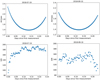 |
Fig. 1 Timesseries of air mass and S/N near 580 nm for the two transits. Data for the first and second transits are shown in the left and right plots, respectively. |
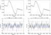 |
Fig. 2 Rossiter–McLaughlin curves and best fit models (upper panel), as well as residuals (lower panels) for the two separate nights (left and right for the first and second transits, respectively). Plots are shown as functions of orbital phase. The sigma values presented on top of each of the lower panels denote the dispersion of the residuals, the fit jitter, and the quadratic sum of the jitter with the average photon noise error, respectively. |
Reference values for the model parameters.
4 The transmission spectrum of HD 209458b
4.1 The fit to the white light RM
Modeling the RM effect implies varying several parameters. Some of them, however, are expected to be color independent. As such, with CARM, we started by fitting the (higher S/N) white-light RVs, that is, the RVs obtained by summing all the CCFs in the full spectrum. These RVs are also used to measure the stellar RV in a given epoch (this is the value that is provided directly by the ESPRESSO DRS). This allows us to fix some of the fit parameters when later adjusting each individual RM curve for a given wavelength regime.
As mentioned above, the full model is comprised of the sum of a Keplerian function and an RM curve. For the latter, we decided to use the AROME code as the baseline, since it allows for the correct modeling of the RVs as derived using the CCF method (see Boué et al. 2013), as well as the use of a quadratic limb-darkening law. The baseline parameters used in this fit, together with their sources, are listed in Table 1. The priors used are listed in Table 2. All parameters not listed were fixed to the values in Table 1.
Some parameters deserve a special note. The value of Vsys depends on the spectrograph and even on the wavelength used. As such, we guessed its value from the values of the observed RV data. The prior we used (see below) is broad enough to be mostly uninformative and allow any uncertainty. The value of σ0 we adopted is the average width of the observed “out-of-transit” CCFs (4.03 km s−1). The central value adopted for v sin i (4.2 km s−1) was taken from a detailed analysis of the ESPRESSO data presented in Casasayas-Barris et al. (in prep.)5. The value is actually half-way between the values derived by Queloz et al. (2000, 3.75 ± 1.25 km s−1), Albrecht et al. (2012, 4.4 ± 0.2 km s−1), and Winn et al. (2005, 4.70 ± 0.16 km s−1). The value ofβ0, which represents the width of the CCF for a nonrotating star, is difficult to derive. As such, we decided to leave it as a free parameter to be fit (see prior discussion below). The macroturbulence parameter (ζt) was derived from the calibration of Doyle et al. (2014), based on the temperature and surface gravity as listed in Table 1. We note that β0, σ0, and ζt are degenerate in the model. Changing their values (individually) would change the measured planet radius. They are, however, supposed to be mostly wavelength independent6. Since in this work we are ultimately interested in variations of radius as functions of wavelength, the zero point of the radius is not relevant. As such, the exact values for these parameters are not critical. Finally, the value of a used as input in AROME is actually given in stellar radius units. We use the values in Table 1 to compute it.
The limb-darkening parameters were set using the LDTK package, and assuming the following stellar parameters listed in the Sweet-Cat database (Santos et al. 2013; Sousa et al. 2018): Teff =6118 K ± 25, log g = 4.36 ± 0.04, [Fe/H] = 0.03 ± 0.02 (their original source is Sousa et al. 2008). The derived values for the linear and quadratic parameters are 0.56 and 0.12, respectively.
For the priors (Table 2), the values used are based on Table 1. For K and Rp, we assumed Gaussian priors with widths three times larger than the listed errors. This takes into account errors in K caused by activity-related noise (not taken into account when fitting the Keplerian) and the fact that the planet radius comes from observations in a different band. For i, λ, and a, we used the values as provided in the literature (Gaussian distributions around the provided value); these values are not supposed to depend on our observational method. For Vsys, we assumed a uniform prior with a broad width of 0.5 km s−1. For the mid-transit time, we propagated the error in T0 and P using the prescription of Kane et al. (2009). The prior on T0 is given by an error margin in phase, Δϕ0.
The value of β0 is more difficult to estimate, since it is not possible to observe it directly. We thus estimated the starting value based on a comparison between the observed width of the CCF in HARPS (3.61 km s−1) and the ESPRESSO (4.03 km s−1) data for HD209458. Using a similar approach as the one presented in Santos et al. (2003), β0 was then estimated as 2.6 km s−1 for HARPS. Accounting (quadratically) for the excess CCF width of the ESPRESSO vs. HARPS7, this allows us to derive a value of β0 for ESPRESSO of 3.2 km s−1. In the model, we adopted a very large, uniform prior around this value (± its absolute value).
Finally, for the additional “jitter” term, we assumed values between 0.0 and 2.5 m s−1. The latter value is five times the observed average photon noise error. This upper limit should take into account any noise coming from stellar oscillations and granulation (e.g., Dumusque et al. 2011), on top of additional instrumental noise that for ESPRESSO are expected to reach ~10 cm s−1 (Pepe et al. 2010).
We note that although the two transits were fit simultaneously, Vsys, Δϕ0, K, and σW were fit independently in the two cases. This allows us to take into account potential variations of these parameters due to, for example, stellar activity effects (it is, e.g., through K that we canmodel longer term trends caused by stellar noise). The resulting values have proven to be similar between the two epochs, even if (as expected) some differences exist. In particular, the values of K and log σW are indistinguishable in both cases (0.083 ± 0.001 km s−1 and − 6.76 ± 0.09 vs. − 6.75 ± 0.09, respectively), while Vsys shows some variation (− 14.7661 ± 0.0002 vs. − 14.7678 ± 0.0002 km s−1). The phase shift Δϕ0 is also slightly different: 0.00078 ± 0.00004 vs. 0.00042 ± 0.00003.
The result of the RM fit to the two transits is presented in Fig. 2. The MCMC was run using a total of 60 walkers (or chains) taken randomly from the priors, allowing them to run for 2000 steps (burn-in) before continuing into the production chains (2000 steps). The fit of the AROME model is computationally intensive8. For some computations, the length of the burn-in phase was insufficient for all the walkers to converge toward the maximum. To avoid non-converged walkers biasing the posterior distributions, we discarded walkers whose posterior value was abnormally lower than that of the rest of the walkers9. Using this approach, we rejected 15 of the 60 walkers from our analysis of the white-light RM curve. The posterior distributions, built from the remaining 90 000 iterations, are presented in Fig. A.1. This plot shows that all parameters converged to distributions that are narrower than the priors.
The median values and their 68% confidence intervals are presented in Table 2. A few of the parameters deserve some comments. First, v sin i converged to a high value (4.8 ± 0.2 km s−1), three-sigma away from the best literature estimate (4.2 ± 0.1 km s−1). As shown in Brown et al. (2017), there is usually a disagreement between the v sin i values derived from the RM fit when compared to those derived from detailed spectroscopic analysis. On its side, β0 converged toward a lower-than-expected value. As can be seen in Fig. A.1, and as expected, β0 and v sin i are highly correlated.
The derived value of λ = 0.6 ± 0.4° (the spin–orbit angle) is closer to the 1.58 ± 0.08° derived by Casasayas-Barris et al. (in prep.), based on the reloaded Rossiter–McLaughlin method (Cegla et al. 2016), than to other literature estimates: − 4.4 ± 1.4° (Winn et al. 2005)and − 5 ± 7° (Albrecht et al. 2012).
Given that ζt is also expected to be strongly correlated with β0 and v sin i, we decided to run the MCMC code again, but to also leave ζt as a free parameter (using a very broad, uniform prior between 0 and 8.8, which is twice the expected value). As a result, we obtained values of β0, v sin i, and ζt of 3.5 ± 0.3 km s−1, 4.6 ± 0.2 km s−1, and  km s−1, respectively.The values for all the remaining variables were, within the error bars, similar to the ones presented in Table 2. We thus conclude that the exact input values for β0, v sin i, and ζt are stronglycorrelated and will not significantly affect the results. We also confirmed that this approach did not change any of the results presented in the next section (i.e., that using a free ζt did not alter the obtained transmission spectrum).
A look at the residuals of the fit to the white-light data (Fig. 2, lower panels) shows some structure, with a peak-to-peak amplitude of ~2 m s−1. In principle,this may be related to uncertainties in the limb-darkening law or in the RM model, as well as to stellar noise produced by, for example, activity crossing events and stellar pulsation. In Di Gloria et al. (2015), the authors corrected this structure using the white-light curve as a proxy for the signal in the different wavelengths. By doing so, they assumed that their residual structure was color independent. Without fully understanding the cause for the observed trends, we preferred, however, not to apply any correction.
Priors used in the white-light fit using AROME as well as the posterior values found.
4.2 The chromatic RM
The next step in our analysis is the derivation of the planet-to-star radius ratio as a function of wavelength. This was done by using the same model as explained in the previous section, but by fitting it to each wavelength interval. In this process, we fixed all parameters that were returned from the white-light RM fit (Table 2), except the systemic velocity of the star10, the noise “jitter” term, and the planet-to-star radius ratio. The priors used for these three parameters are presented in Table 3. For Vsys, we assumed a uniform prior with a width of 0.5 km s−1 around the value from the white-light fit. For Rp∕R⋆, we used a Gaussian prior centered in the value derived from the white-light fit, with an uncertainty of 10%. Finally, for the jitter, we assumed uniform values between 0 m s−1 and the best value coming from the white-light fit multiplied by a (arbitrary) factor of 10. When fitting the two transits simultaneously, Vsys and σW are still fit independently. Finally, the limb-darkening parameters were fixed independently for each wavelength range using the LDTK package.
The minimum wavelength interval for which we can compute RV with the ESPRESSO DRS is the size of one spectral order. When fitting the two transits simultaneously, given that the precision on the RV (derived from the CCF) critically depends on the total S/N of the local spectrum we decided to model the RM signal using two different wavelength binnings: one in steps of four spectral slices and the other in steps of eight slices. The resulting wavelength steps can be seen in Tables B.1 and B.2. Due to the lower S/N of individual data, a binning of eight slices was used when fitting the transits individually. As mentioned above, due to telluric contamination some spectral orders have no CCF and were discarded. In any case, this implies that we do not have a regular spacing in wavelength.
For each wavelength range, the MCMC was run using a total of 30 chains taken randomly from the priors, allowing them to run for 2000steps (burn-in) before continuing into the production chains (2000 steps). An example of an RM fit at 512 nm, as well as the residuals, is presented in Fig. 3.
The median value for the radius derived as a function of wavelength is then used to plot the transmission spectrum (Fig. 4, see also Tables B.1 and B.2). For clarity, we applied an (arbitrary) offset to the values of the radius ratio in all plots, subtracting the value measured in the fourth wavelength bin. In the top panels, we present the spectrum obtained by combining the two transits. The procedure was repeated by analysing each of the two transits separately (bottom panels). This allows us to check if the transmission spectrum we derived is similar in both cases. In all cases, the spectra show the same general trend: a relatively flat region below ~500 nm (0.5 μm), and a bump starting around ~550 nm and finishing after ~700 nm. Above 700 nm, the two spectra show different transmission depths, with the second transit “returning” to values similar to the ones observed in the blue, while the first transit shows significantly lower transmission.
We note, however, that this trend, as it is obtained solely from the second transit, is less pronounced. It is not clear why we observe such a difference in the two transmission spectra as derived independently from the two transits separately. Part of the difference probably results from the lower (and more variable) S/N of the obtained spectra (see Fig. 1). As we see below, during the second night the star was also slightly more active (see next section). However, we cannot exclude instrumental effects or even real variability in the atmosphere of HD 209458b, to explain the observed difference.
Priors used in the chromatic light fit using AROME.
4.3 Testing for robustness
To confirm that the shape of the transmission spectrum did not depend on the RM model used, we performed two further tests.
In the first one, we modeled the RM using the formalism of Ohta et al. (2005), as implemented in PYASTRONOMY. Though this code was built to use RVs derived from a template matching approach (opposite to a CCF method), its can still be used for a consistency check. As discussed above, this software only allows to use a linear limb darkening law. Comparing the two approaches also allows us to verify if the signal we are observing can be due to any wavelength dependent error in the limb darkening laws used.
All priors and parameters used are the same as used above with AROME. Exceptions come from the fact that in this case we do not give as input β0, σ0, and ζt, but we need to include Ω, the angular rotational velocity of the star. We also assumed that the inclination between stellar spin axis and the y-axis is zero, meaning that the input Vrot is equal to vsin i. In Fig. 5, we present a comparison of the transmission spectrum obtained using the two formalisms (using the eight-slice binning). As is clear from the plot, the differences are minor, and always within the errors. We can thus conclude that the shape of the observed transmission spectrum does not depend on the method used to model the RM effect11.
We further decided to redo the fit using the AROME formalisms, but instead of fixing the (quadratic) limb darkening parameters, we let them vary freely for each wavelength bin using uniform priors between 0 and 1, for both the linear and quadratic terms12. The values that were estimated from the white-light fit (0.62 ± 0.13 and 0.36 ± 0.22, respectively for the linear and quadratic term) are reasonably compatible, within the errors, with the ones derived with LDTK (0.56 and 0.12, respectively). The limb-darkening coefficients did not converge in the chromatic curves (due to insufficient S/N of the data). More importantly, the obtained transmission spectrum is very similar to the one obtained with limb-darkening values fixed using LDTK (Fig. 5).
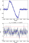 |
Fig. 3 Rossiter–McLaughlin fit to observed signal at 512 nm (top) and residuals (bottom). Data from both transits are phase folded. The Keplerian function was subtracted from the data. |
5 Discussion
In Fig. 6, we compare the transmission spectrum (four-slice binning) we obtained with one derived using HST data and presented in Sing et al. (2016). The data from Sing et al. were compiled from the Exoplanet Atmospheric Spectral Library13. We adopt the dataset version dubbed “2016 Update preferred14”. Due to our uncertainties in the derivation of “absolute” planet radii, in the plot we added an offset to the values of the radius ratio derived using our analysis (subtracting the average difference between our values and those in Sing’s dataset).
A comparison of the two spectra indicates that both show similar trends, even if the ESPRESSO data has lower resolution (due to the spectral binning). In particular, we observe a clear increase in the radius above ~550 nm, an absorption that was identified as being due to Sodium (Sing et al. 2008; Désert et al. 2008). Furthermore, the additional absorption redwards of ~600 nm, already discussed by these authors, is also clearly observed. Désert et al. (2008) suggested that this extra-absorption is possibly due to vanadium oxide (VO) and titanium oxide (TiO) in the atmosphere of HD 209458b. Interestingly, the absorption peaks due to TiO, expected near 620 and 670 nm (see Fig. 3 in Désert et al. 2008), roughly correspond to two of the peaks (higher radius) we observe in the ESPRESSO absorption spectrum. The latter of these two features does not appear in the HST data, and as we will see in Fig. 7, neither is it exactly at the expected wavelength.
It is worth noting that with our dataset, the transmission spectroscopy study of Casasayas-Barris et al. (in prep.) did not manage to detect absorption lines of TiO or VO in high resolution. A similar result concerning TiO was also reported by Hoeijmakers et al. (2015). As highlighted in Hoeijmakers et al. (2015), however, the methods applied imply the use of cross-correlation (“stacking” all individual TiO or VO lines together), and are strongly dependent on the assumption about the expected (model) TiO and VO line spectra.
It is nevertheless interesting that, with an independent dataset and using a different methodology, we observe the same general trend (even if at a lower resolution) that was observed in the 2000 HST dataset. The plot in Fig. 6 also suggests that the additional absorption redwards of ~600 nm may be slightly stronger in the ESPRESSO data when compared with the one observed in the HST dataset. It would be interesting to obtain further observations to confirm if this is a signature of atmospheric variability (see e.g., Parmentier et al. 2013).
Due to telluric contamination, we were not able to obtain transmission data around 700 nm. However, the two reddest wavelength bins show lower values of the planet radius again, compatible with the ones found near 500 nm. Thereddest bin is, however, a bit lower. This point has large error bars and its value should be considered with care. First, its low level mostly comes from the data obtained during the first transit. Also, in the redder part of the spectrum, the number of stellar lines available to compute the RV decreases (the CCF mask used to compute the RV only uses 11 and 15 spectral lines for the two last orders, respectively, when compared to the ~150 in the region near 500 nm). This fact can by itself explain the higher error bars.
It is also worth noting that the peak we tentatively see near 673 nm is close to the Lithium line region (670.7 nm – see Fig. 1 and model of Désert et al. 2008). We note, however, that such feature was not observed in the HST data. Near 460 nm, we also see a small increase in the derived radius, in a region where HST data also shows a small increase (in one single wavelength bin).
The bluest bin in our transmission spectrum is significantly below the remaining ones, and incompatible with the HST data. As we can see from Fig. 4, this decrease is only seen in the second transit. Such behavior could be explained by a spot crossing event or if HD 209458 had a faculae-richer surface by the time of the second transit (Oshagh et al. 2014; Boldt et al. 2020). An estimate of the activity level of the star using the Ca II H and K lines indeed shows a small (but significant) increase in the activity level of the star from the first to the second transit (the value of  changed from − 4.850 ± 0.003 to − 4.840 ± 0.002)15. We should note, however, that this variation is only marginal. The lower S/N in the observed bluest part of the spectrum, with usual values below 30 for the second night (and descending to below ten for the last measurements) is likely a better explanation for the observed discrepancy. Systematic (though difficult to quantify) effects may indeed be expected as we approach the read-out noise limit.
We decided to model the observed transmission spectrum of HD 209458b using the publicly available PLATON code (Zhang et al. 2019, 2020), assuming the recommended prescription with an isothermal atmosphere and equilibrium chemistry. We used the MultiNest approach (with 1000 live points) to fit the data, and used the example that is provided for HD 209458b as a baseline together with the code (see Zhang et al. 2019). We only changed the estimated values of the stellar radius (R⋆ = 1.162 R⊙) and the planet mass (Mp = 0.714 MJup), both from TEP-Cat (Southworth 2010), and the effective temperature of the star, using the value already applied in the RM analysis. A solar C/O ratio of 0.53 was also used; we expect this to be a good approximation given that HD 209458 has solar metallicity (Sousa et al. 2008; Suárez-Andrés et al. 2018). In the fitting procedure, the priors were defined as follows. For R⋆ and Mp, we used Gaussian priors centered in the above-mentioned values and with widths of 0.02R⊙ and 0.04 Mjup, respectively. For the remaining parameters, we used uniform priors: 0.9 × 1.38 < Rp < 1.1 × 1.38 Rjup, 0.5 × 1 459 < Tp < 1.5 × 1 459 K16, − 0.99 < logPtop < 8, − 1< logZ < 3, a multiplicative error factor between 0.5 and 5, and a logarithm of the scattering factor between 0 and 2. We also defined the scattering slope using a pure Rayleigh scattering model, as recommended.
We then tried to fit the data including (or excluding) Na, TiO, and VO, following the example of Désert et al. (2008). A model with no absorption species was also tested as a baseline. Given the uncertainties in the bluest and reddest bins in our data (see above), we decided to exclude these two points from the analysis.
Figure 7 presents some of our results. In Table 4, we also present the natural logarithm of the Bayesian evidence (lnz) of the different models tested. We assume that a model is preferred if this value increases by at least three (Kass & Raftery 1995). As can be seen from the table, models assuming only the Na, TiO, or a combinationof the two, as well as the model with Na, TiO, and VO, all have statistically undistinguishable ln z values. However, all these models are clearly preferred over the “no-elements” model, or the models with only VO or Na + VO.
It is also interesting to see that the best model (highest ln z) is the one thatassumes Na and TiO. The bump observed near 480 nm is reasonably well reproduced by a model including TiO absorption. Interestingly, TiO alone is also able to explain, to the precision level of our data (and to the limits of the model used)the observed transmission spectrum. On the other hand, we find no evidence for the presence of VO absorption.
We should note, however, that none of the models is fully capable of reproducing our dataset, in the sense that in the regions above ~600 nm, our data show an absorption level above the modeled one. The observed mismatch may be caused by modeling approximations (e.g., the isothermal T–P profile), observational errors, effects of stellar activity (e.g., Sedaghati et al. 2017; Espinoza et al. 2019), or by the presence of additional absorbing species such as CaH or ZrO (Van Eck et al. 2017).
In a recent paper, Casasayas-Barris et al. (2020) could not confirm the previous detections of Na absorption as measured at the Na-doublet line cores. They attribute the previous claims to the unaccounted-for Rossiter–McLaughlin effects in the modeling of line profiles. This result has also been confirmed using our ESPRESSO data (Casasayas-Barris et al., in prep.). It may at first sound intriguing that the Na wings may have been detected, while no detectable (within the errors of the ESPRESSO observations and analysis) absorption is measured at the line cores17. Although not conclusive, our result could reinforce the idea that TiO alone may be observed, and that no Na is detected in the atmosphere of HD 209458.
We should note, however, that the methods used in Casasayas-Barris et al. (2020) and in this paper probe the transmission spectrum at very different spectral resolutions. Casasayas-Barris et al. (2020) focus their analysis on the detection of the core of the Na line, and the methodology used does not make it possible to probe broadband variability. On the other hand, in the present study, we are probing broadband variability, thus being sensitive to variations on scales comparable to the expected wings of the Na spectral lines; we are not sensitive to the line core.
Indeed, we could alternatively speculate that the sodium cores may be formed so high in the atmosphere that all Na is ionized, while the wings are formed at a lower temperature region. This could be evidence for the existence of a thermal inversion in the atmosphere of HD 209458b. Although evidence for significant thermal inversion in HD 209458b has not been detected using NIR spectroscopy (e.g., Schwarz et al. 2015), it is interesting to add that TiO has been suggested as a possible source of thermal inversions (Désert et al. 2008; Parmentier et al. 2013; Piette et al. 2020).
To try to test this latter scenario, we decided to rerun PLATON for the models with only Na, only TiO, and Na + TiO, after excluding the two data points near the core of the Na lines. The results show that the ln z, the three models are very similar and statistically undistinguishable. This test is thus inconclusive.
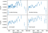 |
Fig. 4 Transmission spectrum of HD 209458 as obtained from the analysis of the chromatic RM curves. The two upper panels showthe combined analysis of the two transits with four- and eight-slice binnings, respectively, for the left and right panels. The two lower panels present the analysis of the two transits separately as computed with an eight-slice binning. |
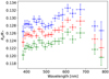 |
Fig. 5 Comparison of derived transmission spectrum using the standard AROME simulation (red), PYASTRONOMY (green), and AROMEwith free limb darkening (blue). For clarity, an arbitrary constant vertical shift was added to the different transmission spectra. |
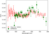 |
Fig. 6 Comparison of the observed transmission spectrum with the one obtained from HST observations and presented in Sing et al. (2016). Green dots correspond to the four-order binning as presented in Fig. 4. |
Logarithm of the Bayesian evidence (ln z) of the different models fit with PLATON.
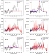 |
Fig. 7 Comparison of our transmission spectrum with synthetic models computed using PLATON. Top: model with “no elements” (left) and with only Na absorption (right). Middle: models with only TiO (left) and with Na + TiO (right). Bottom: models with Na + VO (left) and with all Na, VO, and TiO (right). In all plots, the observational points are denoted in black, with the respective error bars. The red line denotes the best high-spectral resolution model, while the blue points represent its wavelength binned version at the same resolution as the observations. The red shaded area represents the sixteenth and eighty-fourth percentiles of the models. |
6 Conclusions
In this paper, we used ESPRESSO high-resolution spectra to extract the broadband transmission spectrum of HD 209458b, using the chromatic Rossiter-McLaughlin method. We show that the obtained results are compatible with those derived in previous studies using HST data.
We modeled the obtained transmission spectrum using the PLATON software (Zhang et al. 2020). The results suggest that, to the precision level of the data and modeling, either Na + TiO and Na or TiO alone can explain the observed transmission spectrum. However, none of the generated models were fully capable of explaining the observed dataset. More data and a more detailed model may be needed to clarify the exact chemical species responsible for the observed spectrum.
The results presented in this paper show that the application of the chromatic Rossiter-McLaughlin method to ESPRESSO data can be used to set important constraints on the transmission spectrum of exoplanets. With just two transits, we were able to obtain a transmission spectrum of HD 209458b that shows the same structures, albeit at lower resolution, as the one obtained with four HST transits. It will be interesting to apply the same methodology to other targets observed with ESPRESSO.
Acknowledgements
To my grandparents. The authors acknowledge the ESPRESSO project team for its effort and dedication in building the ESPRESSO instrument. This work was supported by FCT - Fundação para a Ciência e a Tecnologia through national funds and by FEDER through COMPETE2020 – Programa Operacional Competitividade e Internacionalização by these grants: UID/FIS/04434/2019; UIDB/04434/2020; UIDP/04434/2020; PTDC/FIS-AST/32113/2017 & POCI-01-0145-FEDER-032113; PTDC/FIS-AST/28953/2017 & POCI-01-0145-FEDER-028953; PTDC/FIS-AST/28987/2017 & POCI-01-0145-FEDER-028987. NJN and VA acknowledge support by FCT through projects reference PTDC/FIS-OUT/29048/2017, IF/00852/2015, and IF/00650/2015/CP1273/CT0001. The INAF authors acknowledge financial support of the Italian Ministry of Education, University, and Research with PRIN 201278X4FL and the “Progetti Premiali” funding scheme. J.H.C.M. is supported in the form of a work contract funded by national funds through FCT (DL 57/2016/CP1364/CT0007). This work has been carried out within the framework of the National Centre of Competence in Research PlanetS supported by the Swiss National Science Foundation. R.A. acknowledgethe financial support of the SNSF. This project has received funding from the European Research Council (ERC) under the European Union’s Horizon 2020 research and innovation programme (project Four Aces grant agreement No 724427). SCCB acknowledges support from Fundação para a Ciência e a Tecnologia (FCT) through Investigador FCT contract IF/01312/2014/CP1215/CT0004. J.P.F. is supported in the form of a work contract funded by national funds through FCT with reference DL57/2016/CP1364/CT0005. ASM acknowledges financial support from the Spanish Ministry of Science and Innovation (MICINN) under the 2019 Juan de la Cierva Programme. A.S.M. acknowledge financial support from the Spanish Ministry of Science, Innovation and Universities (MICIU) AYA2017-86389-P. XD is grateful to The Branco Weiss Fellowship–Society in Science for its financial support. This project has received funding from the European Research Council (ERC) under the European Union’s Horizon 2020 research and innovation programme (project SCORE grant agreement No. 851555) This project has received funding from the European Research Council (ERC) under the European Union’s Horizon 2020 research and innovation programme (project FOUR ACES; grant agreement No 724427). S.G.S acknowledges the support from FCT through Investigador FCT contract nr. CEECIND/00826/2018 and POPH/FSE (EC).
Appendix A Corner plot for the white-light curve
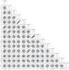 |
Fig. A.1 Corner plot of white-light fit to the two transits. The values and error bars represent the median and 1-sigma uncertainty based on the posterior distributions. The lower right plots for Vsys, Δϕ0, K, and σW concern the second transit. |
Appendix B Data with transmission curves
Planetary radius (in stellar radius units) as a function of wavelength (transmission spectrum) as obtained from our analysis (eight-slice binning).
Planetary radius (in stellar radius units) as a function of wavelength (transmission spectrum), as obtained from our analysis (four-slice binning).
References
- Albrecht, S., Winn, J. N., Johnson, J. A., et al. 2012, ApJ, 757, 18 [NASA ADS] [CrossRef] [Google Scholar]
- Alonso-Floriano, F. J., Snellen, I. A. G., Czesla, S., et al. 2019, A&A, 629, A110 [NASA ADS] [CrossRef] [EDP Sciences] [Google Scholar]
- Astudillo-Defru, N., & Rojo, P. 2013, A&A, 557, A56 [NASA ADS] [CrossRef] [EDP Sciences] [Google Scholar]
- Barros, S. C. C., Demangeon, O., Díaz, R. F., et al. 2020, A&A, 634, A75 [EDP Sciences] [Google Scholar]
- Beaulieu, J. P., Kipping, D. M., Batista, V., et al. 2010, MNRAS, 409, 963 [Google Scholar]
- Boldt, S., Oshagh, M., Dreizler, S., et al. 2020, A&A, 635, A123 [CrossRef] [EDP Sciences] [Google Scholar]
- Bouchy, F., Pepe, F., & Queloz, D. 2001, A&A, 374, 733 [NASA ADS] [CrossRef] [EDP Sciences] [Google Scholar]
- Boué, G., Montalto, M., Boisse, I., Oshagh, M., & Santos, N. C. 2013, A&A, 550, A53 [NASA ADS] [CrossRef] [EDP Sciences] [Google Scholar]
- Brown, D. J. A., Triaud, A. H. M. J., Doyle, A. P., et al. 2017, MNRAS, 464, 810 [Google Scholar]
- Burrows, A. S. 2014, Nature, 513, 345 [Google Scholar]
- Casasayas-Barris, N., Pallé, E., Yan, F., et al. 2020, A&A, 635, A206 [NASA ADS] [CrossRef] [EDP Sciences] [Google Scholar]
- Cegla, H. M., Lovis, C., Bourrier, V., et al. 2016, A&A, 588, A127 [NASA ADS] [CrossRef] [EDP Sciences] [Google Scholar]
- Charbonneau, D., Brown, T., Latham, D., & Mayor, M. 2000, ApJ, 529, L45 [Google Scholar]
- Charbonneau, D., Brown, T. M., Noyes, R. W., & Gilliland, R. L. 2002, ApJ, 568, 377 [Google Scholar]
- Crossfield, I. J. M., Knutson, H., Fortney, J., et al. 2012, ApJ, 752, 81 [Google Scholar]
- Cubillos, P. E., Fossati, L., Koskinen, T., et al. 2020, AJ, 159, 111 [Google Scholar]
- Czesla, S., Schröter, S., Schneider, C. P., et al. 2019, PyA: Python Astronomy-related Packages, Astrophys. Source Code Libr., [record ascl:1906.010] [Google Scholar]
- Deming, D., Seager, S., Richardson, L. J., & Harrington, J. 2005, Nature, 434, 740 [Google Scholar]
- Désert, J. M., Vidal-Madjar, A., Lecavelier Des Etangs, A., et al. 2008, A&A, 492, 585 [NASA ADS] [CrossRef] [EDP Sciences] [Google Scholar]
- Di Gloria, E., Snellen, I. A. G., & Albrecht, S. 2015, A&A, 580, A84 [NASA ADS] [CrossRef] [EDP Sciences] [Google Scholar]
- Dorn, C., Harrison, J. H. D., Bonsor, A., & Hands, T. O. 2019, MNRAS, 484, 712 [Google Scholar]
- Doyle, A. P., Davies, G. R., Smalley, B., Chaplin, W. J., & Elsworth, Y. 2014, MNRAS, 444, 3592 [Google Scholar]
- Dreizler, S., Reiners, A., Homeier, D., & Noll, M. 2009, A&A, 499, 615 [NASA ADS] [CrossRef] [EDP Sciences] [Google Scholar]
- Dumusque, X., Udry, S., Lovis, C., Santos, N. C., & Monteiro, M. J. P. F. G. 2011, A&A, 525, A140 [NASA ADS] [CrossRef] [EDP Sciences] [Google Scholar]
- Ehrenreich, D., Lovis, C., Allart, R., et al. 2020, Nature, 580, 597 [Google Scholar]
- Espinoza, N., Rackham, B. V., Jordán, A., et al. 2019, MNRAS, 482, 2065 [Google Scholar]
- Foreman-Mackey, D., Hogg, D. W., Lang, D., & Goodman, J. 2013, PASP, 125, 306 [Google Scholar]
- Hoeijmakers, H. J., de Kok, R. J., Snellen, I. A. G., et al. 2015, A&A, 575, A20 [NASA ADS] [CrossRef] [EDP Sciences] [Google Scholar]
- Kane, S. R., Mahadevan, S., von Braun, K., Laughlin, G., & Ciardi, D. R. 2009, PASP, 121, 1386 [Google Scholar]
- Kass, R. E., & Raftery, A. E. 1995, J. Am. Stat. Assoc., 90, 773 [CrossRef] [Google Scholar]
- Knutson, H. A., Charbonneau, D., Allen, L. E., Burrows, A., & Megeath, S. T. 2008, ApJ, 673, 526 [Google Scholar]
- Lecavelier Des Etangs, A., Vidal-Madjar, A., Désert, J. M., & Sing, D. 2008, A&A, 485, 865 [NASA ADS] [CrossRef] [EDP Sciences] [Google Scholar]
- Lissauer, J. J., Dawson, R. I., & Tremaine, S. 2014, Nature, 513, 336 [Google Scholar]
- Mayor, M., & Queloz, D. 1995, Nature, 378, 355 [Google Scholar]
- Mayor, M., Lovis, C., & Santos, N. C. 2014, Nature, 513, 328 [Google Scholar]
- McLaughlin, D. B. 1924, ApJ, 60, 22 [Google Scholar]
- Ohta, Y., Taruya, A., & Suto, Y. 2005, ApJ, 622, 1118 [Google Scholar]
- Oshagh, M., Santos, N. C., Ehrenreich, D., et al. 2014, A&A, 568, A99 [NASA ADS] [CrossRef] [EDP Sciences] [Google Scholar]
- Parmentier, V., Showman, A. P., & Lian, Y. 2013, A&A, 558, A91 [NASA ADS] [CrossRef] [EDP Sciences] [Google Scholar]
- Parviainen, H., & Aigrain, S. 2015, MNRAS, 453, 3821 [Google Scholar]
- Pepe, F. A., Cristiani, S., Rebolo Lopez, R., et al. 2010, in SPIE Conf. Ser., 7735 [Google Scholar]
- Pepe, F., Cristiani, S., Rebolo, R., et al. 2020, A&A, in press, https://doi.org/10.1051/0004-6361/202038306 [Google Scholar]
- Piette, A. A. A., Madhusudhan, N., McKemmish, L. K., et al. 2020, MNRAS, 496, 3870 [Google Scholar]
- Queloz, D., Eggenberger, A., Mayor, M., et al. 2000, A&A, 359, L13 [NASA ADS] [Google Scholar]
- Rossiter, R. A. 1924, ApJ, 60, 15 [Google Scholar]
- Rowe, J. F., Matthews, J. M., Seager, S., et al. 2008, ApJ, 689, 1345 [Google Scholar]
- Santos, N. C., Udry, S., Mayor, M., et al. 2003, A&A, 406, 373 [NASA ADS] [CrossRef] [EDP Sciences] [Google Scholar]
- Santos, N. C., Sousa, S. G., Mortier, A., et al. 2013, A&A, 556, A150 [NASA ADS] [CrossRef] [EDP Sciences] [Google Scholar]
- Schneider, J., Dedieu, C., Le Sidaner, P., Savalle, R., & Zolotukhin, I. 2011, A&A, 532, A79 [NASA ADS] [CrossRef] [EDP Sciences] [Google Scholar]
- Schwarz, H., Brogi, M., de Kok, R., Birkby, J., & Snellen, I. 2015, A&A, 576, A111 [NASA ADS] [CrossRef] [EDP Sciences] [Google Scholar]
- Schwartz, J. C., Kashner, Z., Jovmir, D., & Cowan, N. B. 2017, ApJ, 850, 154 [Google Scholar]
- Sedaghati, E., Boffin, H. M. J., MacDonald, R. J., et al. 2017, Nature, 549, 238 [Google Scholar]
- Sing, D. K., Vidal-Madjar, A., Désert, J. M., Lecavelier des Etangs, A., & Ballester, G. 2008, ApJ, 686, 658 [Google Scholar]
- Sing, D. K., Fortney, J. J., Nikolov, N., et al. 2016, Nature, 529, 59 [Google Scholar]
- Snellen, I. A. G. 2004, MNRAS, 353, L1 [Google Scholar]
- Sousa, S. G., Santos, N. C., Mayor, M., et al. 2008, A&A, 487, 373 [NASA ADS] [CrossRef] [EDP Sciences] [MathSciNet] [Google Scholar]
- Sousa, S. G., Adibekyan, V., Delgado-Mena, E., et al. 2018, A&A, 620, A58 [NASA ADS] [CrossRef] [EDP Sciences] [Google Scholar]
- Southworth, J. 2010, MNRAS, 408, 1689 [Google Scholar]
- Suárez-Andrés, L., Israelian, G., González Hernández, J. I., et al. 2018, A&A, 614, A84 [NASA ADS] [CrossRef] [EDP Sciences] [Google Scholar]
- Suárez Mascareño, A., Faria, J. P., Figueira, P., et al. 2020, A&A, 639, A77 [CrossRef] [EDP Sciences] [Google Scholar]
- Swain, M. R., Tinetti, G., Vasisht, G., et al. 2009, ApJ, 704, 1616 [Google Scholar]
- Torres, G., Winn, J. N., & Holman, M. J. 2008, ApJ, 677, 1324 [Google Scholar]
- Van Eck, S., Neyskens, P., Jorissen, A., et al. 2017, A&A, 601, A10 [NASA ADS] [CrossRef] [EDP Sciences] [Google Scholar]
- Vidal-Madjar, A., Lecavelier des Etangs, A., Désert, J.-M., et al. 2003, Nature, 422, 143 [Google Scholar]
- Vidal-Madjar, A., Désert, J.-M., Lecavelier des Etangs, A., et al. 2004, ApJ, 604, L69 [Google Scholar]
- Vidal-Madjar, A., Huitson, C. M., Bourrier, V., et al. 2013, A&A, 560, A54 [NASA ADS] [CrossRef] [EDP Sciences] [Google Scholar]
- Winn, J. N., Noyes, R. W., Holman, M. J., et al. 2005, ApJ, 631, 1215 [Google Scholar]
- Wyttenbach, A., Ehrenreich, D., Lovis, C., Udry, S., & Pepe, F. 2015, A&A 577, A62 [NASA ADS] [CrossRef] [EDP Sciences] [Google Scholar]
- Zellem, R. T., Lewis, N. K., Knutson, H. A., et al. 2014, ApJ, 790, 53 [Google Scholar]
- Zhang, M., Chachan, Y., Kempton, E. M. R., & Knutson, H. A. 2019, PASP, 131, 034501 [Google Scholar]
- Zhang, M., Chachan, Y., Kempton, E. M. R., et al. 2020, ApJ, 899, 27 [Google Scholar]
Based on the reloaded Rossiter–McLaughlin method (e.g., Cegla et al. 2016).
Using a server with 24 cores@2.3 GHz and 128GB RAM: four to five hours for the analysis of the white-light RM curve and a few days for the chromatic analysis performed in Sect. 4.2.
For this purpose, we used the following criteria: ln postwalkeri < median(ln postwalkeri...N) - 3 × MAD(ln postwalkeri...N), where ln postwalkeri is the logarithm of the posterior of walker i, and median(ln postwalkeri...N) and MAD(ln postwalkeri...N) are the median and median absolute deviation of all walkers, respectively.
This is so even if the PYASTRONOMY package is not optimized for the RM modeling of RVs derived using the cross-correlation method (Boué et al. 2013).
All Tables
Priors used in the white-light fit using AROME as well as the posterior values found.
Logarithm of the Bayesian evidence (ln z) of the different models fit with PLATON.
Planetary radius (in stellar radius units) as a function of wavelength (transmission spectrum) as obtained from our analysis (eight-slice binning).
Planetary radius (in stellar radius units) as a function of wavelength (transmission spectrum), as obtained from our analysis (four-slice binning).
All Figures
|
Fig. 1 Timesseries of air mass and S/N near 580 nm for the two transits. Data for the first and second transits are shown in the left and right plots, respectively. |
| In the text | |
|
Fig. 2 Rossiter–McLaughlin curves and best fit models (upper panel), as well as residuals (lower panels) for the two separate nights (left and right for the first and second transits, respectively). Plots are shown as functions of orbital phase. The sigma values presented on top of each of the lower panels denote the dispersion of the residuals, the fit jitter, and the quadratic sum of the jitter with the average photon noise error, respectively. |
| In the text | |
|
Fig. 3 Rossiter–McLaughlin fit to observed signal at 512 nm (top) and residuals (bottom). Data from both transits are phase folded. The Keplerian function was subtracted from the data. |
| In the text | |
|
Fig. 4 Transmission spectrum of HD 209458 as obtained from the analysis of the chromatic RM curves. The two upper panels showthe combined analysis of the two transits with four- and eight-slice binnings, respectively, for the left and right panels. The two lower panels present the analysis of the two transits separately as computed with an eight-slice binning. |
| In the text | |
|
Fig. 5 Comparison of derived transmission spectrum using the standard AROME simulation (red), PYASTRONOMY (green), and AROMEwith free limb darkening (blue). For clarity, an arbitrary constant vertical shift was added to the different transmission spectra. |
| In the text | |
|
Fig. 6 Comparison of the observed transmission spectrum with the one obtained from HST observations and presented in Sing et al. (2016). Green dots correspond to the four-order binning as presented in Fig. 4. |
| In the text | |
|
Fig. 7 Comparison of our transmission spectrum with synthetic models computed using PLATON. Top: model with “no elements” (left) and with only Na absorption (right). Middle: models with only TiO (left) and with Na + TiO (right). Bottom: models with Na + VO (left) and with all Na, VO, and TiO (right). In all plots, the observational points are denoted in black, with the respective error bars. The red line denotes the best high-spectral resolution model, while the blue points represent its wavelength binned version at the same resolution as the observations. The red shaded area represents the sixteenth and eighty-fourth percentiles of the models. |
| In the text | |
|
Fig. A.1 Corner plot of white-light fit to the two transits. The values and error bars represent the median and 1-sigma uncertainty based on the posterior distributions. The lower right plots for Vsys, Δϕ0, K, and σW concern the second transit. |
| In the text | |
Current usage metrics show cumulative count of Article Views (full-text article views including HTML views, PDF and ePub downloads, according to the available data) and Abstracts Views on Vision4Press platform.
Data correspond to usage on the plateform after 2015. The current usage metrics is available 48-96 hours after online publication and is updated daily on week days.
Initial download of the metrics may take a while.