| Issue |
A&A
Volume 644, December 2020
|
|
|---|---|---|
| Article Number | A82 | |
| Number of page(s) | 16 | |
| Section | Interstellar and circumstellar matter | |
| DOI | https://doi.org/10.1051/0004-6361/202039204 | |
| Published online | 02 December 2020 | |
Dense cores in the Seahorse infrared dark cloud: physical properties from modified blackbody fits to the far-infrared–submillimetre spectral energy distributions★
Academy of Finland,
Hakaniemenranta 6, PO Box 131,
00531
Helsinki,
Finland
e-mail: This email address is being protected from spambots. You need JavaScript enabled to view it.
Received:
18
August
2020
Accepted:
4
November
2020
Abstract
Context. Infrared dark clouds (IRDCs) can be the birth sites of high-mass stars, and hence determining the physical properties of dense cores in IRDCs is useful to constrain the initial conditions and theoretical models of high-mass star formation.
Aims. We aim to determine the physical properties of dense cores in the filamentary Seahorse IRDC G304.74+01.32.
Methods. We used data from the Wide-field Infrared Survey Explorer (WISE), Infrared Astronomical Satellite (IRAS), and Herschel in conjuction with our previous 350 and 870 μm observations with the Submillimetre APEX Bolometer Camera (SABOCA) and Large APEX BOlometer CAmera, and constructed the far-IR to submillimetre spectral energy distributions (SEDs) of the cores. The SEDs were fitted using single or two-temperature modified blackbody emission curves to derive the dust temperatures, masses, and luminosities of the cores.
Results. For the 12 analysed cores, which include two IR dark cores (no WISE counterpart), nine IR bright cores, and one H II region, the mean dust temperature of the cold (warm) component, the mass, luminosity, H2 number density, and surface density were derived to be 13.3 ± 1.4 K (47.0 ± 5.0 K), 113 ± 29 M⊙, 192 ± 94 L⊙, (4.3 ± 1.2) × 105 cm−3, and 0.77 ± 0.19 g cm−3, respectively. The H II region IRAS 13039-6108a was found to be the most luminous source in our sample ((1.1 ± 0.4) × 103 L⊙). All the cores were found to be gravitationally bound (i.e. the virial parameter αvir < 2). Two out of the nine analysed IR bright cores (22%) were found to follow an accretion luminosity track under the assumptions that the mass accretion rate is 10−5 M⊙ yr−1, the stellar mass is 10% of the parent core mass, and the radius of the central star is 5 R⊙. Most of the remaing ten cores were found to lie within 1 dex below this accretion luminosity track. Seven out of 12 of the analysed cores (58%) were found to lie above the mass-radius thresholds of high-mass star formation proposed in the literature. The surface densities of Σ > 0.4 g cm−3 derived for these seven cores also exceed the corresponding threshold for high-mass star formation. Five of the analysed cores (42%) show evidence of fragmentation into two components in the SABOCA 350 μm image.
Conclusions. In addition to the H II region source IRAS 13039-6108a, some of the other cores in Seahorse also appear to be capable of giving birth to high-mass stars. The 22 μm dark core SMM 9 is likely to be the youngest source in our sample that has the potential to form a high-mass star (96 ± 23 M⊙ within a radius of ~0.1 pc). The dense core population in the Seahorse IRDC has comparable average properties to the cores in the well-studied Snake IRDC G11.11-0.12 (e.g. Tdust and L agree within a factor of ~1.8); furthermore, the Seahorse, which lies ~60 pc above the Galactic plane, appears to be a smaller (e.g. three times shorter in projection, ~100 times less massive) version of the Snake. The Seahorse core fragmentation mechanisms appear to be heterogenous, including cases of both thermal and non-thermal Jeans instability. High-resolution follow-up studies are required to address the fragmented cores’ genuine potential of forming high-mass stars.
Key words: stars: formation / ISM: clouds / ISM: individual objects: G304.74+01.32 / infrared: ISM / submillimeter: ISM
Based on observations with the Atacama Pathfinder EXperiment (APEX) telescope under programmes 083.F-9302(A) and 089.F-9310(A). APEX is a collaboration between the Max-Planck-Institut für Radioastronomie, the European Southern Observatory, and the Onsala Space Observatory.
© ESO 2020
1 Introduction
Determining the physical properties of dense cores of interstellar molecular clouds is of fundamental importance in the field of star formation research. A powerful method for this purpose is to construct the spectral energy distribution (SED) of the source from observational data obtained at multiple different frequencies (i.e. continuum flux density Sν as a function of frequency ν). In particular, an SED analysis can be used to derive the temperature of the dust component(s), its mass, and also the luminosity over a frequency or wavelength range of interest. The core properties, such as temperature and mass, are central to understanding the initial conditions and early stages of star formation within the parent core.
Of the interstellar molecular clouds that have proved to be fruitful targets for the studies of Galactic star formation, the so-called infrared dark clouds (IRDCs; Pérault et al. 1996; Egan et al. 1998; Simon et al. 2006; Peretto & Fuller 2009) have attracted a lot of interest in recent years (e.g. Tang et al. 2019; Soam et al. 2019; Peretto et al. 2020; Miettinen 2020; Retes-Romero et al. 2020; Moser et al. 2020 to name a few recent studies). Some of the IRDCs studied so far are found to be associated with early stages of high-mass star formation (e.g. Rathborne et al. 2006; Beuther & Steinacker 2007; Chambers et al. 2009; Battersby et al. 2010), and even a few candidates for high-mass prestellar cores have been uncovered in IRDCs (Cyganowski et al. 2014, 2017; Contreras et al. 2018). Therefore, IRDCs are of particular interest in the context of high-mass star formation, where our understanding of the physical mechanisms is still incomplete (e.g. Motte et al. 2018 for a review).
In this paper, we present a study of the physical properties of dense cores in the filamentary IRDC G304.74+01.32, also known as the Seahorse IRDC (Miettinen 2018). The Seahorse IRDC has been fairly well-studied in the submillimetre and millimetre dust continuum emission via single-dish observations (Beltrán et al. 2006; Miettinen & Harju 2010; Miettinen 2018), and through molecular spectral line observations (Miettinen 2012, 2020). Miettinen (2018) derived the dust temperatures of the clumps in the Seahorse IRDC using the 250, 350, and 500 μm peak surface brightness ratios measured with the Spectral and Photometric Imaging Receiver (SPIRE; Griffin et al. 2010) on board the Herschel satellite (Pilbratt et al. 2010)1. Moreover, miettinen2018 determined the masses of the clumps and the cores hosted by the clumps through monochromatic flux densities at 870 and 350 μm, respectively.
To improve the determination of the physical characteristics of the dense core population in the Seahorse IRDC compared to the aforementioned study by miettinen2018, the present study makes use of the source SEDs in the far-IR and submillimetre regime. Moreover, the present study focusses on the usage of data at ~ 9′′−20′′ angular resolution, and does not emply the lower resolution Herschel/SPIRE data. We note that although the SED analysis technique is standard and well established, its application to IRDC substructure samples (cores and clumps) has so far mostly concerned the Galactic plane IRDCs (e.g. Rathborne et al. 2010; Beuther et al. 2010; Henning et al. 2010; Ragan et al. 2012, 2013; Veena et al. 2018), while the Snake IRDC lies about above the Galactic plane.
The core sample and observational data are described in Sect. 2. The analysis and results are described in Sect. 3, and discussed in Sect. 4. Section 5 summarises our results and main conclusions. Throughout this paper, we report the magnitudes in the Vega system and adopt a kinematic distance of d = 2.54 kpc to the Seahorse IRDC (Miettinen 2012, 2018).
2 Source sample and data
The initial source sample of the present study was taken to be the dense cores in the Seahorse IRDC uncovered by Miettinen (2018) through 350 μm dust continuum observations with the Submillimetre APEX BOlometer CAmera (SABOCA; Siringo et al. 2010) at 9′′ (0.11 pc) resolution (full width at half maximum or FWHM). These 17 cores are listed in Table 1.
Miettinen (2018) employed the 3.4, 4.6, 12, and 22 μm IR data from the Wide-field Infrared Survey Explorer (WISE; Wright et al. 2010) to study whether the aforementioned 350 μm cores are associated with embedded young stellar objects (YSOs). We note that because the Seahorse IRDC lies about (~60 pc) above the Galactic plane, it is outside the regions observed with the Spitzer IR satellite (Werner et al. 2004). Five of the 17 cores (29.4%) listed in Table 1 are not associated with WISE sources and are classified as IR dark, while the remaining 12 cores (70.6%) are IR bright. As discussed by Miettinen (2018), the cores SMM 1b and SMM 6b are associated with WISE sources whose IR colours suggest that they could be shock features (see the WISE colour criteria from Koenig et al. 2012; appendix therein), but this would still likely be a sign of ongoing star formation activity in the cores. The WISE source seen towards SMM 7 (6′′ from the 350 μm maximum) was found to be so weak (only detected in the W4 band at 22 μm) that it was interpreted to be a chance projection of a background extragalactic object. However, SMM 7 shows hint of a secondary core (see Appendix A), and the WISE 22 μm source could be associated with it (2′′.8 separation). Hence, in the present study SMM 7 is taken to be an IR bright, star-forming core. The core IRAS 13039-6108a is known to be associated with an optically thin H II region (Sánchez-Monge et al. 2013), and is hence associated with high-mass star formation. We also note that three of the clumps that were detected in the Seahorse IRDC at 870 μm and 19′′. 86 resolution with the Large APEX BOlometer CAmera (LABOCA; Siringo et al. 2009) by Miettinen (2018), namely BLOB 1, SMM 5, and SMM 8, were not detected in our SABOCA map because the emission was resolved out at 9′′ resolution.
To construct the source SEDs, we employed the WISE 22 μm data (12′′ FWHM resolution), and the SABOCA 350 μm and LABOCA 870 μm data from Miettinen (2018). The WISE W4 magnitudes of the sources in the Vega system were taken from the AllWISE catalogue2 (the total in-band brightnesses; see Table 3 in Miettinen 2018), and those were used to compute the 22 μm flux densities by applying the colour corrections under the assumption of a Sν ∝ ν−2 power-law spectrum together with an additional W4 correction (see Cutri et al. 2012). In case the LABOCA 870 μm clump was resolved into two or three cores in our higher resolution SABOCA imaging (SMM 1, SMM 4, IRAS 13037-6112, SMM 6, and IRAS 13039-6108), we used the relative SABOCA 350 μm flux densities of the cores to estimate their contribution to the LABOCA 870 μm emission.
The Seahorse IRDC was observed as part of the Herschel Gould Belt Survey (GBS; André et al. 2010)3. The observations were done with the Photodetector Array Camera and Spectrometer (PACS; Poglitsch et al. 2010) at 70, 100, and 160 μm (~ 9′′, ~ 10′′, and ~ 13′′ resolution, respectively) and with SPIRE at 250, 350, and 500 μm (~ 18′′, ~ 24′′, and ~ 35′′ resolution, respectively). To search for Herschel point source counterparts to the Seahorse cores, we cross-matched our source catalogue with the PACS and SPIRE Point Source Catalogues4 using a search radius of 9′′, that is the beam size of our SABOCA data. Five cores, namely BLOB 2, SMM 4b and 4c, and IRAS 13039-6108a and 13039-6108b were not found to have counterparts in any of the PACS catalogues, and none of the target cores were found to have counterparts in the SPIRE catalogues. However, the Seahorse IRDC as a whole is clearly detected in the SPIRE images as shown in Fig. 2 in Miettinen (2018). Nevertheless, the relatively poor resolution of the SPIRE observations makes those data less useful for the present purpose (e.g. Ragan et al. 2012, 2013), and our SABOCA observations already probed the 350 μm band at 2.7 times higher resolution than SPIRE. We note that the LABOCA clumps BLOB 1, SMM 5, and SMM 8 that were not detected in our SABOCA map also had no matches in the Herschel point source catalogues.
For the three IRAS (Infrared Astronomical Satellite; Neugebauer et al. 1984) sources in the Seahorse we also employed the 25, 60, and 100 μm data from the IRAS Point Source Catalogue v2.15. The angular resolution of IRAS at these wavelengths was about 1′ –2′ (Beichman et al. 1988). For the cores IRAS 13037-6112a and IRAS 13037-6112b we used the WISE 22 μm and PACS 70 and 100 μm data to estimate the cores’ relative contribution to the IRAS flux densities. In the case of the IRAS 13039-6108a/b core pair, all the IRAS emission was assigned to the brighter IRAS 13039-6108a component because it is associated with a 22 μm source while IRAS 13039-6108b is not.
We required that a source needs to have at least three detections in the far-IR and submillimetre regime in addition to the possible WISE 22 μm detection in order to construct a useful source SED for the purpose of the present study. Hence, the final source sample is composed of 12 cores out of which two (SMM 1a and SMM 9) were not detected with WISE and are classified as IR dark cores. The relative percentages of IR bright and IR dark cores in our final sample are therefore 83.3 and 16.7%. The photometric data of these sources are given in Table 2. The PACS 70 μm image towards the Seahorse IRDC is shown in Fig. 1, while panchromatic zoom-in images towards the analysed cores are shown in Fig. A.1.
Initial source sample.
Photometric data of the analysed sources.
3 Analysis and results
3.1 Modified blackbody fits to the SEDs
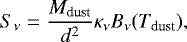
The SEDs of the 12 analysed cores are shown in Fig. 2. Depending on the source, the observed far-IR to submillimetre SEDs were fitted by single or two-temperature modified blackbody functions under the assumption of optically thin dust emission, in which case the general function is given by (e.g. Shetty et al. 2009a,b; Casey 2012; Bianchi 2013)
 (1)
(1)
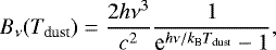
where Mdust is the dust mass, κν is the dust opacity, and Bν (Tdust) is the Planck function at a dust temperature of Tdust defined as
 (2)
(2)
where h is the Planck constant, c is the speed of light, and kB is the Boltzmann constant. The two-temperature component SEDs were fitted with a sum of two modified Planck functions (e.g. Dunne & Eales 2001).
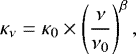
The frequency-dependent dust opacity was assumed to follow a power-law function of the form
 (3)
(3)
where β is the dust emissivity index. We assumed that the κν values followthe Ossenkopf & Henning (1994) dust model values for graphite-silicate dust grains that have coagulated and accreted thin ice mantles over a period of 105 yr at a gas density of nH = 105 cm−3. For reference, the value of κν is 1.38 cm2 g−1 at 870 μm and β ≃ 1.9. The non-linear least squares SED fitting was implemented in Python using the SciPy optimisation module (Virtanen et al. 2020).
The dust masses derived through SED fits were converted to the total gas plus dust masses using a dust-to-gas mass ratio, Rdg = Mdust∕Mgas. The latter value can be derived from the dust-to-hydrogen mass ratio, Mdust∕MH, which is about 1/100 (e.g. Weingartner & Draine 2001; Draine et al. 2007). Assuming that the chemical compositionof the cores is similar to the solar mixture, where the hydrogen mass percentage is X = 71% and those of helium and metals are Y = 27% and Z = 2% (e.g. Anders & Grevesse 1989), the ratio of total gas mass (hydrogen, helium, and metals) to hydrogen gas mass is (X + Y + Z)∕X = 1.41. Based on this assumption, we adopted a dust-to-gas mass ratio of Rdg = 1∕141.
In addition to the dust temperature and mass that were derived through fitting the observed SEDs, we also calculated the bolometric luminosities of the sources by integrating over the fitted SED curves, that is (e.g. Dunham et al. 2010)
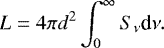 (4)
(4)
To quantify the goodness of the SED fits, we calculated the reduced χ2 values defined as (e.g. Dunham et al. 2006)
 (5)
(5)
where for n data points and m free parameters there are k = n − m degrees of freedom, and the parameters  and
and  are the observed flux densities and their uncertainties and
  is the flux density of the model fit at the corresponding frequency.
The derived SED parameters are listed in Table 3. The quoted uncertainties were derived using the flux density uncertainties. The SED properties of the analysed cores and the derived physical properties of the cores are discussed in Sects. 4.1 and 4.2, respectively.
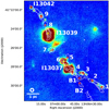 |
Fig. 1 Herschel/PACS 70 μm image towards the IRDC G304.74+01.32 (the Seahorse IRDC). The colour scale is displayed using a linear stretch. The overlaid contours represent the LABOCA 870 μm emission (Miettinen & Harju 2010; Miettinen 2018); the contours start at 3σ, and increase in steps of 3σ, where 3σ = 120 mJy beam−1. The 870 μm clumps are labelled so that the numbers refer to the SMM IDs (e.g. 1 refers to SMM 1), while the sources I13037, I13039, and I13042 are the three IRAS sources in the filament. The sources BLOB 1 and BLOB 2 are labelled as B1 and B2. The plus signs indicate the LABOCA 870 μm emission peaks of the clumps. A scale bar of 1 pc projected length, and the LABOCA beam size (19′′. 86 FWHM) are shown in the bottom left corner. |
3.2 Densities
The volume-averaged H2 number densities of the cores were calculated assuming a spherical geometry and using the formula
 (6)
(6)
where the radii R were taken from Miettinen (2018, Table 2 therein) and they refer to the effective core radius, which is defined as  , where Aproj is the projected area of the core calculated from the total number of pixels that were assigned to the core in the SABOCA map. The quantity
  is the mean molecular weight per H2 molecule, which in our case is
  (Kauffmann et al. 2008, Appendix A.1 therein), and mH is the mass of the hydrogen atom.
We also calculated the surface densities of the cores using the formula
 (7)
(7)
The core radii and derived densities are listed in the last three columns in Table 3. To calculate the values of n(H2) and Σ, we used the sum of the masses of the cold and warm component. The uncertainties in n(H2) and Σ were propagated from the mass uncertainties. The surface densities are plotted as a function of core mass in Fig. 3.
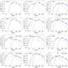 |
Fig. 2 Far-IR to submillimetre SEDs of the analysed cores. Data points at λ ≤ 70 μm are highlighted in red, while the longer wavelength data are shown in blue. The data points shown by green square symbols were not included in the fit (see Sect. 4.1 for details). The downward pointing arrows indicate upper limits (relevant only for some of the IRAS flux densities). The black, dashed lines represent the best modified blackbody fits to the data. For the two-temperature modified blackbody fits, the black, dashed line shows the sum of the two components. The blue and red dashed lines show the SED fits to the cold and warm component, respectively. We note that the y-axis scale is different for the bright IRAS sources compared to the other panels. |
3.3 Virial parameter analysis
To study the dynamical state of the cores, we first calculated their virial masses, Mvir (Bertoldi & McKee 1992). The cores were assumed to be spherical with a radial density profile of the form n(r) ∝ r−p, where the density power-law index, p, was used to calculate the correction factor for the effects of a non-uniform density distribution as described in Appendix A in Bertoldi & McKee (1992). We adopted a value of p = 1.6, which corresponds to the mean value derived by Beuther et al. (2002) for their sample of high-mass star-forming clumps. We note that comparable values were found in other studies of high-mass star-forming clumps and cores (e.g. Mueller et al. 2002: ⟨p⟩ = 1.8 ± 0.4; Garay et al. 2007: p = 1.5−2.2; Zhang et al. 2009: p = 1.6 and p = 2.1 for two cores in the IRDC G28.34+0.06; Li et al. 2019: p = 0.6−2.1 with ⟨p⟩ = 1.3). For example, forthe p values in the range of 1.5−2, a given virial mass varies by 34%.
The total (thermal plus non-thermal), one-dimensional velocity dispersion needed in the calculation of Mvir was calculated as described in Fuller & Myers (1992; see Eq. (3) therein). In this calculation, we assumed that the gas and dust are collisionally coupled and characterised by the same temperature, that is the gas kinetic temperature was taken to be Tkin = Tdust, which is expected to happen at densities n(H2) ≳ 3.2 × 104 cm−3 (Goldsmith 2001). Furthermore, we used the temperature of the cold dust component because it dominates the mass in each target core (see Sect. 4.2).
In the present study, we have adopted a [He]∕[H] abundance ratio of Y∕(4X) = 0.095, which together with the assumption that all hydrogen is molecular leads to a mean molecular weight per free particle of μp = 2.37. We note that the very often used value of μp = 2.33 applies for a[He]∕[H] ratio of 0.1 with no metals (see Kauffmann et al. 2008). As the observed spectral linewidth we used the FWHM of the H13 CO+(J = 2−1) rotational line detected by Miettinen (2020) towards all the parent clumps of the present target cores. The H13 CO+ linewidths were derived through fitting the hyperfine structure of the line, and the critical density of the J =2−1 transition is ncrit = (2.6−3.1) × 106 cm−3 at temperatures between 10 and 20 K (on the basis of the Einstein A coefficient and collision rates given in the Leiden Atomic and Molecular Database (LAMDA6 ; Schöier et al. 2005). Hence, H13 CO+(J = 2−1) is well suited for our purpose as a high-density tracer. In those cases where the Seahore clump is hosting multiple cores (e.g. SMM 1), the same linewidth was adopted for all cores (e.g. for SMM 1a and 1b; see Table 4). We note, however, that the spectral lines on the core scale are expected to be narrower than on the larger clump scale owing to the dissipation of non-thermal, turbulent motions (e.g. Myers 1983; Pineda et al. 2010; Sokolov et al. 2018), and a lower level of gas velocity dispersion would lead to a weaker internal kinetic pressure. The total velocity dispersion also depends on the molecular weight of the observed molecular species, which for H13 CO+ is μmol = 30.
The virial masses of the cores were used to calculate their virial parameters, αvir = Mvir∕M (Bertoldi & McKee 1992; Eq. (2.8a) therein). The value of αvir quantifies the relative importance of the core’s internal kinetic energy and its gravitational energy, and it can be interpreted so that non-magnetised cores with αvir < 2 are gravitationally bound, those with αvir = 1 are in virial equilibrium, and when αvir < 1 the core is gravitationally unstable (e.g. Russeil et al. 2010; Li et al. 2019).
The aforementioned H13 CO+(J = 2−1) linewidths, and the derived virial masses and virial parameters are given in Table 4. The uncertainties in Mvir were propagated from the temperature and linewidth uncertainties, and the uncertainties in αvir were propagated from those of Mvir and M. The values of αvir are plotted as a function of core mass in Fig. 4.
SED parameters and physical properties of the sources.
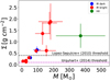 |
Fig. 3 Surface density as a function of core mass. The IR dark cores (no WISE counterpart) are shown by blue data points, while the red data points show the IR bright cores (cores with a WISE counterpart). The H II region IRAS 13037-6112a is indicated by a green data point. The two horizontal dashed lines show the threshold surface densities for high-mass star formation proposed by López-Sepulcre et al. (2010; black) and Urquhart et al. (2014; magenta) when scaled to the present assumptions about the dust properties (see Sect. 4.2). |
H13CO+(J = 2−1) linewidths (FWHM), virial masses, and virial parameters of the cores.
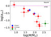 |
Fig. 4 Virial parameter as a function of core mass. The two horizontal dashed lines show the virial equilibrium value (αvir = 1; magenta) and threshold of gravitational boundedness (αvir = 2; black). |
4 Discussion
4.1 Far-infrared to submillimetre SED characteristics of the Seahorse cores
A modified blackbody composed of one or two temperature components is a simplified model for the continuum emission of a dense molecular cloud core. Emission at 22 μm is expected to originate in a warmer dust component closer to the central YSO compared to the colder envelope (see e.g. Beuther et al. 2010; Ragan et al. 2012 for the context of Spitzer 24 μm emission). Hence, a two-temperature model is expected to be a reasonable assumption for the IR bright cores in our sample. Our SED analysis was also based on the assumption of optically thin dust emission, but this assumption might be invalid at 22 μm wavelength. However, adding the dust optical thickness, τ, in Eq. (1) would introduce a third unknown variable (per temperature component) in the problem (Tdust, M, τ), and owing to the fairly low number of data points in our SEDs, the SED fits would start to be subject to overfitting (i.e. number of unknown parameters is comparable to the number of data points).
The angular resolution of the Herschel/PACS data at 70, 100, and 160 μm is 9′′ –13′′, while those of SABOCA and LABOCA are 9′′ and 19′′. 86, respectively.Hence, the resolutions from the PACS to the SABOCA wavelength are similar within a factor of 1.4, and even the LABOCA resolution is only 2.2 times lower than the highest resolution (9′′) data used in the SED fits. However, the IRAS data have a much lower angular resolution compared to our other data, but the corresponding flux densities still appear to be in fairly good agreement with other measurements (see below).
As shown in Fig. 2, a one or two-temperature modified blackbody could be well-fitted to the SEDs of the 22 μm dark cores SMM 1a and SMM 9, and also to the SEDs of the 22 μm bright, YSO hosting cores SMM 1b, 4a, 6a, and IRAS 13037-6112a, 13037-6112b, 13039-6108a, and 13042-6105. Of the aforementioned cores, SMM 1a was the only source where a single-temperature model was fitted to the observed SED. In the case of SMM 4a and SMM 6a, the number of flux density data points is equal to the number of free parameters of the two-component model, and hence there are zero degrees of freedom. Hence, the value of  of the best-fit SED for these two sources is infinite.
For the 22 μm bright cores SMM 2 and SMM 7, the observed 22 μm flux density is not consistent with a two-temperature model fit, which could be an indication of the presence of another, still warmer dust component, or of the failure of the assumptions used in the analysis, for example that of optically thin dust emission. Moreover, for the 22 μm bright core SMM 3, a two-temperature model fit yielded two overlapping modified Planck curves that appeared similar to the single-temperature model fit shown in Fig. 2. We opted for the single-temperature fit because it yielded a much lower  value (8.21) than the poor two-temperature fit (
 ). Also in the case of SMM 3 a more complex model might be need to explain its 22 μm emission (more than two dust components or optically thick 22 μm emisson or both), but we note that the 70 μm data point was not available for SMM 3 so a direct comparison with the cases of SMM 2 and SMM 7 is not feasible.
The SED of IRAS 13037-6112b could not be successfully fit with a two-temperature model when the IRAS 60 μm flux density data point was included in the fit. Hence, we decided to omit that data point from the fit, and this choice was further supported by the presence of a PACS 70 μm data point that was measured at a much higher (factor of ~7) angular resolution than the IRAS 60 μm data point. For IRAS 13037-6112a, however, a two-temperature model could be fitted even when the 60 μm data point was included in the fit, although the best-fit model is in much better agreement with the PACS 70 μm data point. As seen in the SEDs of the IRAS sources, the WISE 22 μm and IRAS 25 μm flux densities arein agreement with each other, where the latter are 1.5–1.6 times higher. For IRAS 13039-6108a, a two-temperature model could not fit the IRAS100 μm data point, and hence we opted for an SED fit where that data point is omitted (the  value of the fit also dropped from 9.25 to 3.77 when the 100 μm data point was not used in the fit). We note that for IRAS 13039-6108a, which is associated with an H II region, no counterparts were found from the PACS Point Source Catalogue, which is probably the result of the extended source appearance at the PACS wavelengths (70–160 μm; Fig. A.1). This could explain the high IRAS 100 μm flux density of the source. The source is also extended and associated with diffuse emission region in the WISE 12 and 22 μm images as shown in Fig. 3 in Miettinen (2018) and Fig. A.1 herein, which is consistent with the H II region state of source evolution where a photodissociation region is surrounding the ionised gas bubble. We also note that for IRAS 13037-6112a, 13037-6112b, and 13042-6105, the SED fits are consistent with the IRAS flux density upper limits.
One could argue that the adopted Ossenkopf & Henning (1994) dust model of grains with thin ice mantles is not valid for the warm dust component. For example, the adopted dust opacities in a wavelength range of 20–100 μm, which typically brackets the peak of the warm SED component, are on average about 1.6 ± 0.1 times higherthan those in the corresponding model of grains without ice mantles. Nevertheless, the usage of the Ossenkopf & Henning (1994) model of bare dust particles with no icy coverages would basically only lead to about 1.6 times higher masses of the warm dust component. Because the latter masses are so low compared to the cold component (Mwarm∕Mcold = 1 × 10⁻⁴ − 0.03 with a mean of 5 × 10⁻³), the usage of the thin ice mantle based parameters seems justified also for the warm component.
4.2 Physical properties of the Seahorse cores and the potential for high-mass star formation
The mean (median) values of the derived dust temperatures of the cold component, core masses, luminosities, number densities, and surface densities are 13.3 ± 1.4 K (12.6 K), 113 ± 29 M⊙ (94 M⊙), 192 ± 94 L⊙ (62 L⊙), (4.3 ± 1.2) × 105 cm−3 (2.8 × 105 cm−3), and 0.77 ± 0.19 g cm−2 (0.61 g cm−2). The mean (median) dust temperature and mass of the warm component are 47.0 ± 5.0 K (50.7 K) and 0.6 ± 0.3 M⊙ (0.1 M⊙). As mentioned in Sect. 4.1, the mass of the warm component is only 5 per mille of the cold component’s mass on average (the median Mwarm∕Mcold ratio is 2.5 × 10⁻³). As expected, the H II region source IRAS 13039-6108a was found to be the most luminous source in our sample (L = (1.1 ± 0.4) × 103 L⊙), but surprisingly the second lowest dust temperature of the cold component in our sample was derived for IRAS 13039-6108a (Tdust = 8.3 ± 1.3 K). IRAS 13039-6108a also does not show the highest warm component temperature in our sample, but there are five cores that are still warmer (51.2−64.0 K compared to 50.2 K for IRAS 13039-6108a).
In Fig. 5, we plot the core luminosity as a function of core mass. The black dashed line plotted in Fig. 5 indicates the accretion luminosity defined as
 (8)
(8)
where Ṁacc is the mass accretion rate and M⋆ and R⋆ are the mass and radius of the central star. Following Ragan et al. (2012, Fig. 14 therein), we assumed that Ṁacc = 10−5 M⊙ yr−1, the stellar mass is 10% of the parent core mass, and that R⋆ = 5 R⊙. In general, the YSO evolution in the L−M diagram shown in Fig. 5 occurs towards the top left corner (i.e. the parent core or envelope mass decreases while the luminosity increases; e.g. Saraceno et al. 1996; Molinari et al. 2008). Two IR bright cores in our sample lie close (within a factor of ~ 1.4) to the aforementioned accretion luminosity trend. Also, the H II region IRAS 13039-6108a lies only a factor of 2 below that trend line. Most of the remaining cores lie clearly below that trend, for example the two 22 μm dark cores lie approximately one dex below the trend, which could be an indication of a lower mass accretion rate (and/or lower stellar mass and larger central star). Only IRAS 13037-6112a is found to lie (by a factor of 2.9) above the Lacc line corresponding to an accretion rate of 10−5 M⊙ yr−1. The latter rate is not sufficient to overcome the radiation pressure barrier of high-mass star formation, which requires values of Ṁacc > 10−4 M⊙ yr−1, and indeed such high values have been derived for high-mass star-forming objects (e.g. Zinnecker & Yorke 2007; Motte et al. 2018 for reviews, and references therein). See Sect. 4.3 for further discussion.
Figure 6 shows the core masses as a function of their effective radius. For comparison, the magenta dashed line plotted in the figure shows the empirical mass-radius threshold for high-mass star formation proposed by Kauffmann & Pillai (2010); see also Kauffmann et al. (2010a). We note that the authors also used the Ossenkopf & Henning (1994) dust opacities for grains with thin ice mantles coagulating for 105 yr, but the model density was assumed to be 106 cm−3 rather than 105 cm−3 as we did. In a wavelength range of 350 μm–1 mm, the former dust opacities are on average 1.285 ± 0.002 times higherthan our values. Moreover, Kauffmann & Pillai (2010) decreased the opacities by a factor of 1.5 to calibrate between the dust extinction and dust emission based mass estimates (see Kauffmann et al. 2010b for details). We used the original Ossenkopf & Henning (1994) opacities and a factor of 1.41 higher gas-to-dust mass ratio than what seems to have been used in the reference studies of Kauffmann & Pillai (2010). Taking these differences into account, theKauffmann & Pillai (2010) threshold relationship for high-mass star formation can be written as
 (9)
(9)
Seven out of our 12 cores (58%) lie above the Kauffmann & Pillai (2010) threshold for high-mass star formation. These include five IR bright cores, the H II region IRAS 13039-6108a, and the 22 μm dark core SMM 9, where IRAS 13039-6108a lies furthest above the threshold, that is by a factor of 4.8 ± 2.0. Moreover, the IR bright core SMM 3 and IR dark core SMM 1a lie very close to this critical threshold, namely a factor of 1.09 ± 0.19 and 1.03 ± 0.15 below it, respectively.
Baldeschi et al. (2017) also derived an empirical mass-radius threshold relationship for high-mass star formation (see their Eq. (9)). The authors assumed that the opacity at 300 μm is 0.1 cm2 g−1, which includes a dust-to-gas mass ratio of 1/100. When scaled to our corresponding assumptions, the Baldeschi et al. (2017) threshold becomes
 (10)
(10)
As illustrated in Fig. 6, the Baldeschi et al. (2017) threshold lies above the Kauffmann & Pillai (2010) threshold by  . All the seven cores that lie above the Kauffmann & Pillai (2010) threshold, also lie above the Baldeschi et al. (2017) threshold. For example, IRAS 13039-6108a fulfils the latter criterion by lying a factor of 3.5 ± 1.5 above it.
As illustrated in Fig. 4, all the target cores appear to be gravitationally bound (αvir < 2). We note that the 22 μm dark cores SMM 1a and SMM 9 could harbour YSO(s) that are too weak to be detected with WISE (e.g. the 5σ point-source sensitivity in the W4 band is 5.4 mJy; Wright et al. 2010), and indeed the PACS 70 μm observations suggest that the cores already have an ongoing central heating (although the 70 μm counterpart of SMM 1a could not be found from the PACS catalogue; see Appendix A). The other way round, SMM 1a and SMM 9 are unlikely to be prestellar cores.
To quantitatively estimate the mass of the most massive star that could form in the target cores, we used the Kroupa (2001) stellar initial mass function based formula from Svoboda et al. (2016, their Eq. (10); see also Sanhueza et al. 2017, appendix therein), which is given by
 (11)
(11)
where ɛSF is the star formation efficiency (SFE). Adopting a value of ɛSF = 0.3 (e.g. Lada & Lada 2003 for a review; Alves et al. 2007), Eq. (11) yields maximum stellar masses of  M⊙ for the IR bright cores, 2.0 ± 0.2 M⊙ and 3.1 ± 0.6 M⊙ for the 22 μm dark cores SMM 1a and SMM 9, and 8.9 ± 2.9 M⊙ for IRAS 13039-6108a. This suggests that the IR bright and IR dark cores in the Seahorse IRDC could give birth to multiple systems of low-mass stars (~ 0.1−2 M⊙) or intermediate-mass stars (~ 2−8 M⊙) rather than collapse to form a massive star of at least 8 M⊙, which only seems to be the case in the already known high-mass star-forming object IRAS 13039-6108a. We note that according to Eq. (11), high-mass star formation requires at least a 320 M⊙ core for ɛSF = 0.3. On the other hand, in the competitive accretion paradigm the cores like SMM 1a and SMM 1b could competitively accrete more mass from their parent clump SMM 1, and this process has the potential to lead to the formation of a massive star at the centre of the gravitational potential well (e.g. Bonnell & Bate 2006).
To further assess our core sample’s potential for high-mass star formation, in Fig. 3 we plot their surface densities as a function of core mass. For comparison, two threshold surface densities for high-mass star formation are also shown in Fig. 3. López-Sepulcre et al. (2010) determined an empirical surface density threshold for massive star formation of Σthres = 0.3 g cm−2 on the basis of the outflow characteristics of their sample. The authors assumed that the dust opacity is 1 cm2 g−1 at 1.2 mm and that Rdg = 1∕100. When scaled to the present assumptions, the López-Sepulcre et al. (2010) surface density threshold becomes Σthres = 0.4 g cm−2. On the other hand, on the basis of a large sample of ~ 1 700 massive YSOs in ~ 1 300 clumps drawn from the APEX Telescope Large Area Survey of the Galaxy (ATLASGAL; Schuller et al. 2009), Urquhart et al. (2014) found that a surface density of 0.05 g cm−2 might set a minimum threshold for high-mass star formation. Again, when taking into account that Urquhart et al. (2014) assumed different dust properties than we (κ870 μm = 1.85 cm2 g−1 and Rdg = 1∕100), we scaled their reported surface density threshold to 0.095 g cm−2. Seven (58%) of the target cores lie above the López-Sepulcre et al. (2010) threshold by factors of 1.5 ± 0.2 − 4.7 ± 2.0. The latter percentage is the same as for the cores that fulfil the Kauffmann & Pillai (2010) and Baldeschi et al. (2017) thresholds for high-mass star formation (the cores in question are the same in both cases). All the cores are found to lie above the Urquhart et al. (2014) threshold by factors of 1.3 ± 0.6 − 19.8 ± 8.3, where five cores lie in between the two Σthres values.
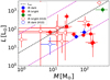 |
Fig. 5 Core luminosity plotted against the core mass. For comparison, a sample of ten IR dark and IR bright cores in the Snake IRDC from Henning et al. (2010) are shown with empty circles (see Sect. 4.3 and Appendix B). The black dashed line shows the accretion luminosity with a mass accretion rate of Ṁacc = 10−5 M⊙ yr−1 and assuming a stellar mass of M⋆ = 0.1 × Mcore and stellar radius of R⋆ = 5 R⊙ (see Eq. (8)). The magenta dashed lines above and below the aforementioned line show a ± 1 dex variation of the accretion luminosity in question. |
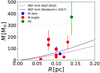 |
Fig. 6 Core mass plotted against the effective core radius. The magenta and black dashed lines indicate the empirical mass-radius thresholds for high-mass star formation proposed by Kauffmann & Pillai (2010) and Baldeschi et al. (2017), respectively. When scaled to the assumptions adopted in the present study, these thresholds are given by
|


4.3 Comparison with the properties of dense cores in the Snake IRDC
As discussed in Miettinen (2018), the Seahorse IRDC shares some similarities with the Snake IRDC G11.11-0.12. Both the clouds are filamentary in their projected morphology, and they appear to have been hierarchically fragmented into substructures (e.g. Ragan et al. 2015). Altogether 17 cores were detected with SABOCA in the Seahorse IRDC, and three LABOCA clumps (SMM 5, SMM 8, and BLOB 1) were resolved out in the SABOCA map (Miettinen 2018). Because 14 of these 20 sources are associated with a WISE 22 μm source, the percentage of 22 μm bright cores is 70% ± 19%, where the quoted uncertainty represents the Poisson error on counting statistics (here, SMM 7 is counted as IR bright opposite to the studies by Miettinen 2018, 2020; see Table 1 and Appendix A). Henning et al. (2010) found that 11 out of their 18 cores that are found along the Snake filament are associated with Spitzer 24 μm emission, which makes the percentage of IR bright cores 61% ± 18%, which is comparable to that in the Seahorse. Accounting for the off-filament cores in the Snake, the aforementioned percentage becomes even more similar to ours (i.e. 67% ± 17%; Henning et al. 2010, Table 1 therein). The differences are that the Snake IRDC lies at a distance of 3.6 kpc (i.e. a factor of 1.4 further away than the Seahorse) and has a projected length of about 30 pc, and it is also very massive, ~ 105 M⊙ (Kainulainen et al. 2013; Lin et al. 2017). The Seahorse filament is about 9 pc long and has a mass of ~ 103 M⊙ (Miettinen 2018).
We note that Henning et al. (2010) applied a similar SED analysis to derive the Snake IRDC’s core properties as in the present study (i.e. modifed blackbody fitting), and hence we took their sample as our main comparison sample of IRDC cores.However, for a better comparison with the present results, we re-analysed the SEDs of the Snake IRDC cores using the same method and assumptions as in the present study (see Appendix B for details).
In Fig. 7, we show the distributions of dust temperature, mass, and luminosity of the cores in both the Seahorse IRDC and the Snake IRDC, where the latter values are listed in Table B.1 (the ten out of 18 on-filament sources for which SED analysis could be done). The mean (median) values of these quantities for the Snake cores are  K (19 K),
  K (50 K), ⟨M⟩ = 49 ± 28 M⊙ (14 M⊙), and ⟨L⟩ = 349 ± 267 L⊙ (71 L⊙). These values are 1.5 ± 0.2 (1.5), 1.1 ± 0.1 (1.0), 0.4 ± 0.3 (0.1), and 1.8 ± 1.6 (1.2) times those for the Seahorse cores (see Sect. 4.2). The Snake cores appear somewhat warmer (in the cold component), less massive (by a factor of 2.5 ± 1.9 on average),and about 80% more luminous on average (while the median luminosities differ by only a factor of 1.2). However, at least partly these differences can be attributed to our inclusion of the longer wavelength data (350 and 870 μm), which leads to lower temperatures of the cold componenent (hence higher mass).
Interestingly, also the Snake IRDC contains one IR bright core, the P1 core (i.e. core no. 9), with a luminosity of about  L⊙, which is comparable (
 times larger) to that we derived for IRAS 13039-6108a. The Snake P1 also has a mass similar to that of IRAS 13039-6108a (a factor of 1.3 ± 0.6 difference). We note that the Snake P1 is known to be associaated with 6.7 GHz Class II methanol (CH3OH) maser and 22 GHz water (H2O) maser emission, which are signposts of high-mass star formation (Pillai et al. 2006; Wang et al. 2014).
In Fig. 5, we also plot the luminosities and masses of the analysed core sample in the Snake IRDC filament. Three out of the nine IR bright Snake cores (33.3%) lie close (within a factor of 1.5) to the line of accretion luminosity with Ṁacc = 10−5 M⊙ yr−1, although we note that the associated uncertainties are large. This is comparable to the corresponding percentage in our sample, that is two out of nine (22%) IR bright cores lie within a factor of ~ 1.4 of the trend; see Sect. 4.2. The one analysed IR dark core in the Snake filament lies within 1 dex below the aforementioned L − M relationship, just like the two IR (22 μm) dark cores in our sample. Overall, the Seahorse and Snake cores’ properties suggest that the Seahorse and Snake IRDCs are in comparable evolutionary stages, at least in terms of their star formation phase.
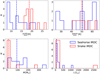 |
Fig. 7 Distributions of dust temperature, mass, and luminosity of the cores in the Seahorse IRDC (blue histogram; present study) and Snake IRDC (red histogram; Henning et al. 2010; Appendix B herein). The vertical dashed lines indicate the sample medians. |
4.4 Core fragmentation
In the paper by Miettinen (2018), we studied the fragmention of the clumps in the Seahorse IRDC into cores, and in this section we address the fragmention of the cores into still smaller units. As discussed in Appendix A, five out of the 12 analysed cores (42%) show evidence of fragmentation in the SABOCA 350 μm image. The observed, projected separations between the fragments range from 0.09 pc in SMM 7 to 0.21 pc in SMM 4a. We note that all these systems were extracted as single sources in the source extraction analysis by Miettinen (2018).
The observed fragment separations can be compared with the thermal Jeans length of the core,  (e.g. McKee & Ostriker 2007 for a review, Eq. (20) therein). Again, we assumed that Tkin = Tdust (for the cold component), and the mass density needed in the calculation was defined as
  to be consistent with Eq. (6). The thermal Jeans mass of the cores was calculated using the definition in McKee & Ostriker (2007), that is
  .
.
The SED based core masses were compared with the Jeans mass by calculating the Jeans number, NJ = M∕MJ. The aforementioned fragmentation parameters are listed in Table 5. The uncertainties in the parameters were propagated from those in the temperature, density, and mass.
As seen in Table 5, the observed fragment separation in SMM 6a is comparable to its thermal Jeans length (the ratio between the two is 1.4 ± 0.3). For the remaining four cores, the observed fragment separation is 3.0 ± 0.2 to 6.4 ± 1.4 times the thermal Jeans length, which could be an indication that the derived temperature of the cold dust component underestimates the parent core temperature(e.g. 8.3 ± 1.3 K for IRAS 13039-6108a seems very low) or that also non-thermal motions contribute to the Jeans instability. For these sources, we also calculated the Jeans length where the thermal sound speed, cs, is replaced by the effective sound speed defined as  (e.g. Bonazzola et al. 1987; Mac Low & Klessen 2004 for a review). The one-dimensional non-thermal velocity dispersion is often written under the assumption of isotropicity as
  with vrms the three-dimensional, rms turbulent velocity. Using the H13 CO+(J = 2−1) linewidths (Col. 2 in Table 4), the effective sound speed increases the Jeans lenghts in SMM 1a, 4a, and 7 and IRAS 13039-6108a to 0.14 pc, 0.11 pc, 0.03 pc, and 0.06 pc, respectively. These are 1.5–3 times the corresponding thermal Jeans lengths, and 33–74% of the observed fragment separation. We note that magnetic pressure would also contribute to the effective sound speed (e.g. McKee & Tan 2003), and could also contribute to the core fragmentation.
As seen in Col. 6 in Table 5, the cores contain multiple thermal Jeans masses, although the Jeans numbers are associated with significant uncertainties. The highest Jeans numbers are found for SMM 1a, 4a, and 7 and IRAS 13039-6108a, but those would be decreased by factors of 3.4–21 (e.g. to NJ = 163 ± 145 for IRAS 13039-6108a) if the non-thermal Jeans lengths are used to derive the corresponding Jeans masses. Nevertheless, it is possible that the studied cores are fragmented into multiple condensations and this hypothesis can be tested by high-resolution observations with telescopes like Atacama Large Millimetre/submillimetre Array (ALMA; Wootten & Thompson 2009).
In conclusions, the analysed cores exhibit heterogeneous fragmentation properties so that SMM 6a is consistent with pure thermal Jeans fragmentation, while the other four cores listed in Table 5 appear to require additional mechanism(s) in their fragmentation in addition to gravity and thermal pressure support. Despite the physical mechanisms of how the cores were fragmented, their physical properties derived from the SEDs should be interpreted as those of the systems of at least two fragments, and this has direct consequence to the cores’ ability to form either massive stars or multiple stellar systems.
Core fragment separations and the Jeans analysis parameters.
5 Summary and conclusions
We used data from the WISE, IRAS, and Herschel satellites together with our previous submillimetre dust continuum observations with the APEX telescope to construct the far-IR to submillimetre SEDs of the SABOCA 350 μm selected cores in the Seahorse IRDC G304.74+01.32. The SEDs were fitted using single and two-temperature modified blackbody models. Ourmain results are summarised as follows:
- 1.
For the 12 analysed cores, out of which two are IR dark (no WISE detection), the mean values of the derived dust temperatures for the cold (warm) component, masses, luminosities, H2 number densities, and surface densities were found to be 13.3 ± 1.4 K (47.0 ± 5.0 K), 113 ± 29 M⊙, 192 ± 94 L⊙, (4.3 ± 1.2) × 105 cm−3, and 0.77 ± 0.19 g cm−2. All the cores in our sample were found to be gravitationally bound (αvir < 2).
- 2.
The most luminous source (L = (1.1 ± 0.4) × 103 L⊙) in our sample was found to be IRAS 13039-6108a, which is known to be in the H II region stage of evolution.
- 3.
Two out of the nine analysed IR bright cores (22%) were found to have luminosities that are consistent with the accretion luminosity where the mass accretion rate was assumed to be 10−5 M⊙ yr−1, the stellar mass was fixed at 10% of the parent core mass, and the radius of the central star was assumed to be 5 R⊙. Most of the remaining cores (6 out of 10) were found to lie within 1 dex below the aforementioned accretion luminosity value.
- 4.
Seven out of the 12 analysed cores (58%) were found to lie above the mass-radius thresholds of high-mass star formation presented by Kauffmann & Pillai (2010) and Baldeschi et al. (2017). The same seven cores were derived to have mass surface densities of >0.4 g cm−3 that also make them potential high-mass star-forming cores. Hence, in addition to IRAS 13039-6108a, the Seahorse IRDC is potentially hosting substructures capable of forming high-mass stars.
- 5.
The average dust temperatures and luminosities of dense cores in the Seahorse IRDC were found to be fairly similar (within a factor of ~1.8) to those in the well-studied Snake IRDC G11.11-0.12, which is also known to host a high-mass star-forming object (the P1 region) and a number of lower mass cores. The Snake cores were found to be about 2.5 times less massive on average than the Seahorse cores, but at least part of the aforementioned differences can be explained by the fact that we also included the available submillimetre wavelength data in the SED fits of the Seahorse cores.
- 6.
Five out of the 12 analysed cores (42%; SMM 1a, 4a, 6a, 7, and IRAS 13039-6108a) show evidence of fragmentation in the SABOCA 350 μm image, and the fragment separation in SMM 6a is consistent with thermal Jeans fragmentation (i.e. dsep = (1.4 ± 0.3) × λJ), while the other four cores appear to require non-thermal fragmentation processes.
Although the Seahorse IRDC lies about or ~60 pc above the Galactic plane, it appears to have comparable star-forming properties to the Spitzer-selected filamentary IRDCs in or closer to the Galactic plane. More detailed studies of the Seahorse core fragments and implications for the cores’ ability to form massive stars require high-resolution follow-up observations. In particular, (sub-)millimetre dust continuum and molecular spectral line imaging of the cores with instruments like ALMA would be the next natural step in studying the Seahorse IRDC filament.
Acknowledgements
I would like to thank the anonymous referee for providing comments and suggestions. This research has made use of NASA’s Astrophysics Data System Bibliographic Services, the NASA/IPAC Infrared Science Archive, which is operated by the Jet Propulsion Laboratory, California Institute of Technology, under contract with the National Aeronautics and Space Administration, and Astropy (http://www.astropy.org), a community-developed core Python package for Astronomy (Astropy Collaboration 2013, 2018). This publication makes use of data products from the Wide-field Infrared Survey Explorer, which is a joint project of the University of California, Los Angeles, and the Jet Propulsion Laboratory/California Institute of Technology, and NEOWISE, which is a project of the Jet Propulsion Laboratory/California Institute of Technology. WISE and NEOWISE are funded by the National Aeronautics and Space Administration.
Appendix A Multiwavelength images of the analysed cores and the source appearances
In Fig. A.1, we show the WISE 12 and 22 μm and Herschel/PACS 70 and 100 μm images towards the analysed cores. Each image is overlaid with contours showing the SABOCA 350 μm and LABOCA 870 μm dust continuum emission. Selected sources are discussed below.
The WISE source J130622.27-613014.7 seen towards SMM 1 appears to lie in between the SABOCA cores SMM 1a and SMM 1b. The WISE source is interpreted to be associated with SMM 1b, where the projected separation between the two is 8′′. 9. Also, the colours of the WISE source suggest that it could be related to shock emission (Miettinen 2018), which could explain the fairly large distance from SMM 1b. Nevertheless, this would still be an indication that SMM 1b is a star-formingcore. On the other hand, the WISE source could also be associated with the SMM 1a’s subcondensation (5′′. 95 separation) 15′′. 3 to the east of the stronger SABOCA 350 μm peak. The core SMM 1a itself is classified as IR dark because it has no WISE counterpart. However, SMM 1a is not 70 μm dark as illustrated in Fig. A.1 although the PACS Point Source Catalogue did not contain a corresponding counterpart.
The WISE source J130637.23-612848.8 seen towards SMM 3 appears weak in the 12 and 22 μm images, but it can be found in the AllWISE catalogue. The PACS 70 μm source is well coincident with the WISE source’s catalogue position as shown in Fig. A.1. There are also two other PACS sources to the east and south-west of SMM 3, both of which are visible in the WISE images, and there is weak (3σ) SABOCA 350 μm emission seen towards the former source.
The source WISE J130646.35-612855.3, which is assigned to SMM 4a, is not detected in the W3 (12 μm) band of WISE (> 9.344 mag), and it is also not obviously seen in the 22 μm image although the AllWISE catalogue contains such detection (W4 = 6.001 ± 0.233 mag). The core SMM 4a also appears to contain a subcondensation 16′′.8 to the south-west of the brighter component. This subcondensation also appears in the PACS images and is hence a real source, and an indication that SMM 4a is fragmented. The parent clump SMM 4 appears to contain multiple SABOCA sources and the system is likely a formation site of a stellar group or cluster.
We note that the WISE source seen 29′′.4 to the west of WISE J130651.93-612822.2 associated with IRAS 13037-6112a, is the source WISE J130647.85-612819.5 associated with SMM 4b. Also, the images towards IRAS 13037-6112 shown in Fig. A.1 contain the SABOCA cores SMM 6a and 6b in the northern part of the images (cf. the SMM 6 panels).
The core SMM 6a shows an additional condensation 12′′.7 to the south-west of the stronger peak position. The WISE source J130654.93-612725.9 is associated with the latter position (see the 12 μm image in Fig. A.1). The WISE source J130652.20-612735.0 associated with SMM 6b is not clearly visible in the WISE 12 and 22 μm images shown in Fig. A.1, but the AllWISE catalogue reported a detection in all the four bands W1–W4 (3.4–22 μm). The source WISE J130652.20-612735.0 has WISE colours in between an embedded YSO and a shock feature (Miettinen 2018), but there is a PACS 100 μm source 5′′.4 away from the WISE source, which suggests that it could be a YSO.
In our previous studies of the Seahorse IRDC (Miettinen 2018, 2020), the WISE source J130704.50-612620.6 seen towards SMM 7 (6′′ offset) was considered a background extragalactic object, namely a star-forming galaxy or an active galactic nucleus, because the colours of this weak WISE source were suggestive of its extragalactic nature and the source is only detected at 22 μm. However, SMM 7 shows a hint of an additional SABOCA 350 μm peak 7′′. 5 to the south of the brighter SABOCA peak, and WISE J130704.50-612620.6 could in fact be an embedded YSO associated with this secondary SABOCA peak (2′′.8 projected offset). The latter source position is coincident with the PACS far-IR emission. Hence, in the present work we take SMM 7 to be an IR bright core.
IRAS 13039-6108a, which is associated with the WISE source J130707.22-612438.5 (7′′. 7 separation), shows another SABOCA 350 μm fragment 13′′.4 to the north of the emission maximum. There is also an extension of SABOCA 350 μm emission to the west of IRAS 13039-6108a. This H II region is extended in the WISE 12 μm and 22 μm images, which suggests the presence of a photodissociation region.
There isa WISE source in the AllWISE catalogue that is seen towards SMM 9. However, it is not identifiable in the WISE 12 and 22 μm images shown in Fig. A.1, and indeed it is reported to be undetected at 12 μm in the AllWISE catalogue (W3 > 10.159 mag). This source, WISE J130713.09-612238.2, lies 9′′.1 from the SABOCA 350 μm peak position of SMM 9, and its WISE colours suggest that it is a foreground star rather than an embedded YSO (Miettinen 2018). Hence, SMM 9 is taken to be IR dark but the source is detected with PACS at 70 μm.
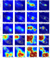 |
Fig. A.1 Multiwavelength images towards the target cores (WISE 12 and 22 μm and Herschel/PACS 70 and 100 μm). The WISE images are shown with logarithmic scaling except the 22 μm images of SMM 7 and SMM 9 that are shown with power-law scaling to enhance the colour contrast. The PACS images are displayed using a linear stretch. In each panel, the overlaid yellow contours show the SABOCA 350 μm dust continuum emission and the white contours show the LABOCA 870 μm emission. The contour levels start from 3σ, and progressin steps of 1σ, where 1σ = 200 mJy beam−1 for the SABOCA data and 1σ = 40 mJy beam−1 for the LABOCA data (Miettinen 2018). Each image is centred on the LABOCA peak position of the parent clump, and is 60′′ × 60′′ in size with the exception of the IRAS 13037 and IRAS 13039 images, which are 85′′ on a side. In those cases where the LABOCA clump contains more than one SABOCA core (e.g. components a and b), the crosses indicate the 350 μm peak positions of the cores. The red diamond symbols show the WISE source positions (see Miettinen 2018, Table 3 therein). The plus sign in the IRAS 13039 image indicates the position of the 18 and 22.8 GHz radio continuum source found by Sánchez-Monge et al. (2013). A scale bar of 0.25 pc is shown in each panel. |
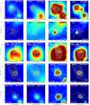 |
Fig. A.1 continued. |
Appendix B SED analysis of dense cores in the Snake IRDC
Similarly to the present study, Henning et al. (2010) also used modifed blackbody SED fitting technique to derive the Snake IRDC’s coreproperties. However, the difference is that while we used two-temperature modifed blackbodies to fit the WISE 22 μm data point, Henning et al. (2010) did not inlucde the Spitzer/MIPS (Multiband Imaging Photometer for Spitzer; Rieke et al. 2004) 24 μm data in the SED fitting because the corresponding emission might be optically thick. Instead, the authors fit the Herschel/PACS data only and also neglected the longer wavelength data, for example those measured with Herschel/SPIRE owing to its coarser resolution, which prevented the identification of the PACS cores.
For better comparison with the present results, we fit the SEDs of the cores in the Snake IRDC filament following the same method as outlined in Sect. 3.1. We note that the Spitzer and Herschel/PACS photometric data used by Henning et al. (2010) were not reported by the authors, and hence we serched for the photometric data from the MIPSGAL (MIPS Galactic Plane Survey; Carey et al. 2009) Catalogue7 and the PACS Point Source Catalogues. As a search radius, we used 10′′ with respect to the coordinates given in Table 1 in Henning et al. (2010). When the PACS 70 or 100 μm photometricdata could not be found from the PACS Point Source Catalogues, we searched for the data from the Hi-GAL (the Herschel infrared Galactic Plane Survey; Molinari et al. 2016) 70 and 100 μm Photometric Catalogues8.
For the Snake core 3, no photometric data were found at all from the aforementioned catalogues, and for the cores 6, 7, 11, 14, and 17 only two photometric data points were found, and hence their SEDs were not analysed. We note that there is a MIPS 24 μm source, namely MG011.1545-00.1688, which lies 5′′.8 away from core 7. However, Henning et al. (2010) reported the core to be 24 μm dark (the two photometric data points we found from the Herschel catalogues were those at 70 and 100 μm). On the other hand, no MIPS 24 μm counterpart was found for core 13 (within 10′′) although it was reported to be 24 μm bright by Henning et al. (2010). Also, the PACS data of this core could not be successfully fit with our modifed blackbody model. For core 12, three photometric data points were found, but one of them was at 24 μm (the other two being 70 and 160 μm), and hence the wavelength coverage was not sufficient for the present SED analysis. Hence, among the cores 1–18 in the Snake IRDC filament (Henning et al. 2010, Table 1 therein), we could analyse ten cores. Of these ten cores, only one (core 1) is 24 μm dark.
The derived SED parameters for the ten analysed cores in the Snake IRDC are listed in Table B.1. Two example SEDs are plotted in Fig. B.1. For three of the cores (1, 2, and 4), the data were fitted with a single-temperature model. Of these, core 1 is 24 μm dark and had only the three PACS data points to fit. For core 2, our two-temperature model could not fit the 24 μm data point, and hence we fit the PACS data only with a single-temperature model. This is a similar case as SMM 3 in the Seahore IRDC (see Fig. 2). For core 4, we did not find a MIPS 24 μm counterpart but Henning et al. (2010) reported the core to be associated with a 24 μm source. The PACS data of core 4 were fitted with a single-temperature model. The SEDs of the remaining seven cores listed in Table B.1 were fitted with a two-temperature model.
The dust temperatures (of the cold component), core masses, and luminosities we derived for the Snake cores are about 0.7–1.2, 0.1–19, and 1.0–3.1 times the values reported by Henning et al. (2010). On average, our analysis yielded about 0.8, 3.2, and 2.2 times the temperature, mass, and luminosity values from Henning et al. (2010). For example, the difference in the luminosity values is caused by the inclusion of the Spitzer 24 μm data in our SED fitting. We note that Henning et al. (2010) adopted a dust opacity of 1 cm2 g−1 at 850 μm with Rgd = 1∕100. In the Ossenkopf & Henning (1994) dust model adopted in the present work, the 850 μm dust opacity would be about 1.44 cm2 g−1, which together with our 1.41 times lower dust-to-gas mass ratio yield a factor of 0.98 to scale the core masses from Henning et al. (2010) to be consistent with our assumptions. Because this factor is so close to unity, we used the original core masses reported by Henning et al. (2010) in the above comparison.
SED parameters of dense cores in the Snake IRDC.
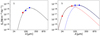 |
Fig. B.1 Two examples of SEDs of dense cores in the Snake IRDC. Core 1 (left panel) is 24 μm dark, while core 5 (right panel) is associated with a 24 μm source. Datapoints at λ ≤ 70 μm are highlighted in red, while the longer wavelength data are shown in blue. The black, dashed lines represent the best modified blackbody fits to the data. For core 5, the latter represents the sum of the cold and warm components, where the individual fits are shown by the blue and red dashed lines, respectively. |
References
- Alves, J., Lombardi, M., & Lada, C. J. 2007, A&A, 462, L17 [NASA ADS] [CrossRef] [EDP Sciences] [Google Scholar]
- Anders, E., & Grevesse, N. 1989, Geochim. Cosmochim. Acta, 53, 197 [Google Scholar]
- André, Ph., Men’shchikov, A., Bontemps, S., et al. 2010, A&A, 518, L102 [NASA ADS] [CrossRef] [EDP Sciences] [Google Scholar]
- Astropy Collaboration (Robitaille, T. P., et al.) 2013, A&A, 558, A33 [NASA ADS] [CrossRef] [EDP Sciences] [Google Scholar]
- Astropy Collaboration (Price-Whelan, A. M., et al.) 2018, AJ, 156, 123 [Google Scholar]
- Baldeschi, A., Elia, D., Molinari, S., et al. 2017, MNRAS, 466, 3682 [NASA ADS] [CrossRef] [Google Scholar]
- Battersby, C., Bally, J., Jackson, J. M., et al. 2010, ApJ, 721, 222 [NASA ADS] [CrossRef] [Google Scholar]
- Beichman, C. A., Neugebauer, G., Habing, H. J., et al. 1988, Infrared Astronomical Satellite (IRAS) Catalogs and Atlases. Vol. 1: Explanatory Supplement, 1 [Google Scholar]
- Beltrán, M. T., Brand, J., Cesaroni, R., et al. 2006, A&A, 447, 221 [NASA ADS] [CrossRef] [EDP Sciences] [MathSciNet] [Google Scholar]
- Bertoldi, F., & McKee, C. F. 1992, ApJ, 395, 140 [NASA ADS] [CrossRef] [Google Scholar]
- Beuther, H., & Steinacker, J. 2007, ApJ, 656, L85 [NASA ADS] [CrossRef] [Google Scholar]
- Beuther, H., Schilke, P., Menten, K. M., et al. 2002, ApJ, 566, 945 [NASA ADS] [CrossRef] [Google Scholar]
- Beuther, H., Henning, T., Linz, H., et al. 2010, A&A, 518, L78 [NASA ADS] [CrossRef] [EDP Sciences] [Google Scholar]
- Bianchi, S. 2013, A&A, 552, A89 [NASA ADS] [CrossRef] [EDP Sciences] [Google Scholar]
- Bonazzola, S., Heyvaerts, J., Falgarone, E., et al. 1987, A&A, 172, 293 [Google Scholar]
- Bonnell, I. A., & Bate, M. R. 2006, MNRAS, 370, 488 [NASA ADS] [CrossRef] [Google Scholar]
- Carey, S. J., Noriega-Crespo, A., Mizuno, D. R., et al. 2009, PASP, 121, 76 [NASA ADS] [CrossRef] [Google Scholar]
- Casey, C. M. 2012, MNRAS, 425, 3094 [Google Scholar]
- Chambers, E. T., Jackson, J. M., Rathborne, J. M., et al. 2009, ApJS, 181, 360 [NASA ADS] [CrossRef] [Google Scholar]
- Contreras, Y., Sanhueza, P., Jackson, J. M., et al. 2018, ApJ, 861, 14 [NASA ADS] [CrossRef] [Google Scholar]
- Cutri, R. M., Wright, E. L., Conrow, T., et al. 2012, Explanatory Supplement to the WISE All-Sky Data Release Products, http://wise2.ipac.caltech.edu/docs/release/allsky/expsup/index.html [Google Scholar]
- Cyganowski, C. J., Brogan, C. L., Hunter, T. R., et al. 2014, ApJ, 796, L2 [NASA ADS] [CrossRef] [Google Scholar]
- Cyganowski, C. J., Brogan, C. L., Hunter, T. R., et al. 2017, MNRAS, 468, 3694 [NASA ADS] [CrossRef] [Google Scholar]
- Draine, B. T., Dale, D. A., Bendo, G., et al. 2007, ApJ, 663, 866 [NASA ADS] [CrossRef] [Google Scholar]
- Dunham, M. M., Evans, N. J., Bourke, T. L., et al. 2006, ApJ, 651, 945 [NASA ADS] [CrossRef] [Google Scholar]
- Dunham, M. M., Evans, N. J., Terebey, S., et al. 2010, ApJ, 710, 470 [NASA ADS] [CrossRef] [Google Scholar]
- Dunne, L., & Eales, S. A. 2001, MNRAS, 327, 697 [NASA ADS] [CrossRef] [Google Scholar]
- Egan, M. P., Shipman, R. F., Price, S. D., et al. 1998, ApJ, 494, L199 [NASA ADS] [CrossRef] [Google Scholar]
- Fuller, G. A., & Myers, P. C. 1992, ApJ, 384, 523 [Google Scholar]
- Garay, G., Mardones, D., Brooks, K. J., et al. 2007, ApJ, 666, 309 [NASA ADS] [CrossRef] [Google Scholar]
- Goldsmith, P. F. 2001, ApJ, 557, 736 [NASA ADS] [CrossRef] [MathSciNet] [Google Scholar]
- Griffin, M. J., Abergel, A., Abreu, A., et al. 2010, A&A, 518, L3 [EDP Sciences] [Google Scholar]
- Güsten, R., Nyman, L. Å., Schilke, P., et al. 2006, A&A, 454, L13 [NASA ADS] [CrossRef] [EDP Sciences] [Google Scholar]
- Henning, T., Linz, H., Krause, O., et al. 2010, A&A, 518, L95 [NASA ADS] [CrossRef] [EDP Sciences] [Google Scholar]
- Kainulainen, J., Ragan, S. E., Henning, T., et al. 2013, A&A, 557, A120 [NASA ADS] [CrossRef] [EDP Sciences] [Google Scholar]
- Kauffmann, J., & Pillai, T. 2010, ApJ, 723, L7 [NASA ADS] [CrossRef] [Google Scholar]
- Kauffmann, J., Bertoldi, F., Bourke, T. L., et al. 2008, A&A, 487, 993 [NASA ADS] [CrossRef] [EDP Sciences] [Google Scholar]
- Kauffmann, J., Pillai, T., Shetty, R., et al. 2010a, ApJ, 716, 433 [NASA ADS] [CrossRef] [Google Scholar]
- Kauffmann, J., Pillai, T., Shetty, R., et al. 2010b, ApJ, 712, 1137 [NASA ADS] [CrossRef] [Google Scholar]
- Koenig, X. P., Leisawitz, D. T., Benford, D. J., et al. 2012, ApJ, 744, 130 [NASA ADS] [CrossRef] [Google Scholar]
- Kroupa, P. 2001, MNRAS, 322, 231 [NASA ADS] [CrossRef] [Google Scholar]
- Lada, C. J., & Lada, E. A. 2003, ARA&A, 41, 57 [NASA ADS] [CrossRef] [Google Scholar]
- Li, S., Zhang, Q., Pillai, T., et al. 2019, ApJ, 886, 130 [NASA ADS] [CrossRef] [Google Scholar]
- Lin, Y., Liu, H. B., Dale, J. E., et al. 2017, ApJ, 840, 22 [NASA ADS] [CrossRef] [Google Scholar]
- López-Sepulcre, A., Cesaroni, R., & Walmsley, C. M. 2010, A&A, 517, A66 [NASA ADS] [CrossRef] [EDP Sciences] [Google Scholar]
- Mac Low, M.-M., & Klessen, R. S. 2004, Rev. Mod. Phys., 76, 125 [NASA ADS] [CrossRef] [Google Scholar]
- McKee, C. F., & Ostriker, E. C. 2007, ARA&A, 45, 565 [NASA ADS] [CrossRef] [Google Scholar]
- McKee, C. F., & Tan, J. C. 2003, ApJ, 585, 850 [NASA ADS] [CrossRef] [MathSciNet] [Google Scholar]
- Miettinen, O. 2012, A&A, 540, A104 [NASA ADS] [CrossRef] [EDP Sciences] [Google Scholar]
- Miettinen, O. 2018, A&A, 609, A123 [NASA ADS] [CrossRef] [EDP Sciences] [Google Scholar]
- Miettinen, O. 2020, A&A, 639, A65 [CrossRef] [EDP Sciences] [Google Scholar]
- Miettinen, O., & Harju, J. 2010, A&A, 520, A102 [NASA ADS] [CrossRef] [EDP Sciences] [Google Scholar]
- Molinari, S., Pezzuto, S., Cesaroni, R., et al. 2008, A&A, 481, 345 [NASA ADS] [CrossRef] [EDP Sciences] [Google Scholar]
- Molinari, S., Schisano, E., Elia, D., et al. 2016, A&A, 591, A149 [NASA ADS] [CrossRef] [EDP Sciences] [Google Scholar]
- Moser, E., Liu, M., Tan, J. C., et al. 2020, ApJ, 897, 136 [CrossRef] [Google Scholar]
- Motte, F., Bontemps, S., & Louvet, F. 2018, ARA&A, 56, 41 [NASA ADS] [CrossRef] [Google Scholar]
- Mueller, K. E., Shirley, Y. L., Evans, N. J., et al. 2002, ApJS, 143, 469 [NASA ADS] [CrossRef] [Google Scholar]
- Myers, P. C. 1983, ApJ, 270, 105 [NASA ADS] [CrossRef] [Google Scholar]
- Neugebauer, G., Habing, H. J., van Duinen, R., et al. 1984, ApJ, 278, L1 [Google Scholar]
- Ossenkopf, V., & Henning, T. 1994, A&A, 291, 943 [NASA ADS] [Google Scholar]
- Pérault, M., Omont, A., Simon, G., et al. 1996, A&A, 315, L165 [Google Scholar]
- Peretto, N., & Fuller, G. A. 2009, A&A, 505, 405 [NASA ADS] [CrossRef] [EDP Sciences] [Google Scholar]
- Peretto, N., Rigby, A., André, P., et al. 2020, MNRAS, 496, 3482 [CrossRef] [Google Scholar]
- Pillai, T., Wyrowski, F., Carey, S. J., et al. 2006, A&A, 450, 569 [NASA ADS] [CrossRef] [EDP Sciences] [Google Scholar]
- Pilbratt, G. L., Riedinger, J. R., Passvogel, T., et al. 2010, A&A, 518, L1 [CrossRef] [EDP Sciences] [Google Scholar]
- Pineda, J. E., Goodman, A. A., Arce, H. G., et al. 2010, ApJ, 712, L116 [Google Scholar]
- Poglitsch, A., Waelkens, C., Geis, N., et al. 2010, A&A, 518, L2 [NASA ADS] [CrossRef] [EDP Sciences] [Google Scholar]
- Ragan, S., Henning, T., Krause, O., et al. 2012, A&A, 547, A49 [NASA ADS] [CrossRef] [EDP Sciences] [Google Scholar]
- Ragan, S. E., Henning, T., & Beuther, H. 2013, A&A, 559, A79 [NASA ADS] [CrossRef] [EDP Sciences] [Google Scholar]
- Ragan, S. E., Henning, T., Beuther, H., et al. 2015, A&A, 573, A119 [NASA ADS] [CrossRef] [EDP Sciences] [Google Scholar]
- Rathborne, J. M., Jackson, J. M., & Simon, R. 2006, ApJ, 641, 389 [NASA ADS] [CrossRef] [Google Scholar]
- Rathborne, J. M., Jackson, J. M., Chambers, E. T., et al. 2010, ApJ, 715, 310 [NASA ADS] [CrossRef] [Google Scholar]
- Retes-Romero, R., Mayya, Y. D., Luna, A., et al. 2020, ApJ, 897, 53 [CrossRef] [Google Scholar]
- Rieke, G. H., Young, E. T., Engelbracht, C. W., et al. 2004, ApJS, 154, 25 [NASA ADS] [CrossRef] [Google Scholar]
- Russeil, D., Zavagno, A., Motte, F., et al. 2010, A&A, 515, A55 [NASA ADS] [CrossRef] [EDP Sciences] [Google Scholar]
- Sánchez-Monge, Á., Beltrán, M. T., Cesaroni, R., et al. 2013, A&A, 550, A21 [NASA ADS] [CrossRef] [EDP Sciences] [Google Scholar]
- Sanhueza, P., Jackson, J. M., Zhang, Q., et al. 2017, ApJ, 841, 97 [NASA ADS] [CrossRef] [Google Scholar]
- Saraceno, P., Andre, Ph., Ceccarelli, C., et al. 1996, A&A, 309, 827 [Google Scholar]
- Schuller, F., Menten, K. M., Contreras, Y., et al. 2009, A&A, 504, 415 [NASA ADS] [CrossRef] [EDP Sciences] [Google Scholar]
- Schöier, F. L., van der Tak, F. F. S., van Dishoeck, E. F., et al. 2005, A&A, 432, 369 [NASA ADS] [CrossRef] [EDP Sciences] [Google Scholar]
- Shetty, R., Kauffmann, J., Schnee, S., et al. 2009a, ApJ, 696, 676 [NASA ADS] [CrossRef] [Google Scholar]
- Shetty, R., Kauffmann, J., Schnee, S., et al. 2009b, ApJ, 696, 2234 [NASA ADS] [CrossRef] [Google Scholar]
- Simon, R., Jackson, J. M., Rathborne, J. M., et al. 2006, ApJ, 639, 227 [NASA ADS] [CrossRef] [Google Scholar]
- Siringo, G., Kreysa, E., Kovács, A., et al. 2009, A&A, 497, 945 [NASA ADS] [CrossRef] [EDP Sciences] [Google Scholar]
- Siringo, G., Kreysa, E., De Breuck, C., et al. 2010, The Messenger, 139, 20 [NASA ADS] [Google Scholar]
- Soam, A., Liu, T., Andersson, B.-G., et al. 2019, ApJ, 883, 95 [CrossRef] [Google Scholar]
- Sokolov, V., Wang, K., Pineda, J. E., et al. 2018, A&A, 611, L3 [CrossRef] [EDP Sciences] [Google Scholar]
- Svoboda, B. E., Shirley, Y. L., Battersby, C., et al. 2016, ApJ, 822, 59 [NASA ADS] [CrossRef] [Google Scholar]
- Tang, Y.-W., Koch, P. M., Peretto, N., et al. 2019, ApJ, 878, 10 [CrossRef] [Google Scholar]
- Urquhart, J. S., Moore, T. J. T., Csengeri, T., et al. 2014, MNRAS, 443, 1555 [NASA ADS] [CrossRef] [Google Scholar]
- Veena, V. S., Vig, S., Mookerjea, B., et al. 2018, ApJ, 852, 93 [NASA ADS] [CrossRef] [Google Scholar]
- Virtanen, P., Gommers, R., Oliphant, T. E., et al. 2020, Nat. Methods, 17, 261 [Google Scholar]
- Wang, K., Zhang, Q., Testi, L., et al. 2014, MNRAS, 439, 3275 [NASA ADS] [CrossRef] [Google Scholar]
- Weingartner, J. C., & Draine, B. T. 2001, ApJ, 548, 296 [NASA ADS] [CrossRef] [Google Scholar]
- Werner, M. W., Roellig, T. L., Low, F. J., et al. 2004, ApJS, 154, 1 [NASA ADS] [CrossRef] [Google Scholar]
- Wootten, A., & Thompson, A. R. 2009, IEEE Proc., 97, 1463 [NASA ADS] [CrossRef] [Google Scholar]
- Wright, E. L., Eisenhardt, P. R. M., Mainzer, A. K., et al. 2010, AJ, 140, 1868 [Google Scholar]
- Zhang, Q., Wang, Y., Pillai, T., et al. 2009, ApJ, 696, 268 [NASA ADS] [CrossRef] [Google Scholar]
- Zinnecker, H., & Yorke, H. W. 2007, ARA&A, 45, 481 [NASA ADS] [CrossRef] [Google Scholar]
Herschel is an ESA space observatory with science instruments provided by European-led Principal Investigator consortia and with important participation from NASA.
All Tables
H13CO+(J = 2−1) linewidths (FWHM), virial masses, and virial parameters of the cores.
All Figures
|
Fig. 1 Herschel/PACS 70 μm image towards the IRDC G304.74+01.32 (the Seahorse IRDC). The colour scale is displayed using a linear stretch. The overlaid contours represent the LABOCA 870 μm emission (Miettinen & Harju 2010; Miettinen 2018); the contours start at 3σ, and increase in steps of 3σ, where 3σ = 120 mJy beam−1. The 870 μm clumps are labelled so that the numbers refer to the SMM IDs (e.g. 1 refers to SMM 1), while the sources I13037, I13039, and I13042 are the three IRAS sources in the filament. The sources BLOB 1 and BLOB 2 are labelled as B1 and B2. The plus signs indicate the LABOCA 870 μm emission peaks of the clumps. A scale bar of 1 pc projected length, and the LABOCA beam size (19′′. 86 FWHM) are shown in the bottom left corner. |
| In the text | |
|
Fig. 2 Far-IR to submillimetre SEDs of the analysed cores. Data points at λ ≤ 70 μm are highlighted in red, while the longer wavelength data are shown in blue. The data points shown by green square symbols were not included in the fit (see Sect. 4.1 for details). The downward pointing arrows indicate upper limits (relevant only for some of the IRAS flux densities). The black, dashed lines represent the best modified blackbody fits to the data. For the two-temperature modified blackbody fits, the black, dashed line shows the sum of the two components. The blue and red dashed lines show the SED fits to the cold and warm component, respectively. We note that the y-axis scale is different for the bright IRAS sources compared to the other panels. |
| In the text | |
|
Fig. 3 Surface density as a function of core mass. The IR dark cores (no WISE counterpart) are shown by blue data points, while the red data points show the IR bright cores (cores with a WISE counterpart). The H II region IRAS 13037-6112a is indicated by a green data point. The two horizontal dashed lines show the threshold surface densities for high-mass star formation proposed by López-Sepulcre et al. (2010; black) and Urquhart et al. (2014; magenta) when scaled to the present assumptions about the dust properties (see Sect. 4.2). |
| In the text | |
|
Fig. 4 Virial parameter as a function of core mass. The two horizontal dashed lines show the virial equilibrium value (αvir = 1; magenta) and threshold of gravitational boundedness (αvir = 2; black). |
| In the text | |
|
Fig. 5 Core luminosity plotted against the core mass. For comparison, a sample of ten IR dark and IR bright cores in the Snake IRDC from Henning et al. (2010) are shown with empty circles (see Sect. 4.3 and Appendix B). The black dashed line shows the accretion luminosity with a mass accretion rate of Ṁacc = 10−5 M⊙ yr−1 and assuming a stellar mass of M⋆ = 0.1 × Mcore and stellar radius of R⋆ = 5 R⊙ (see Eq. (8)). The magenta dashed lines above and below the aforementioned line show a ± 1 dex variation of the accretion luminosity in question. |
| In the text | |
|
Fig. 6 Core mass plotted against the effective core radius. The magenta and black dashed lines indicate the empirical mass-radius thresholds for high-mass star formation proposed by Kauffmann & Pillai (2010) and Baldeschi et al. (2017), respectively. When scaled to the assumptions adopted in the present study, these thresholds are given by
|
| In the text | |
|
Fig. 7 Distributions of dust temperature, mass, and luminosity of the cores in the Seahorse IRDC (blue histogram; present study) and Snake IRDC (red histogram; Henning et al. 2010; Appendix B herein). The vertical dashed lines indicate the sample medians. |
| In the text | |
|
Fig. A.1 Multiwavelength images towards the target cores (WISE 12 and 22 μm and Herschel/PACS 70 and 100 μm). The WISE images are shown with logarithmic scaling except the 22 μm images of SMM 7 and SMM 9 that are shown with power-law scaling to enhance the colour contrast. The PACS images are displayed using a linear stretch. In each panel, the overlaid yellow contours show the SABOCA 350 μm dust continuum emission and the white contours show the LABOCA 870 μm emission. The contour levels start from 3σ, and progressin steps of 1σ, where 1σ = 200 mJy beam−1 for the SABOCA data and 1σ = 40 mJy beam−1 for the LABOCA data (Miettinen 2018). Each image is centred on the LABOCA peak position of the parent clump, and is 60′′ × 60′′ in size with the exception of the IRAS 13037 and IRAS 13039 images, which are 85′′ on a side. In those cases where the LABOCA clump contains more than one SABOCA core (e.g. components a and b), the crosses indicate the 350 μm peak positions of the cores. The red diamond symbols show the WISE source positions (see Miettinen 2018, Table 3 therein). The plus sign in the IRAS 13039 image indicates the position of the 18 and 22.8 GHz radio continuum source found by Sánchez-Monge et al. (2013). A scale bar of 0.25 pc is shown in each panel. |
| In the text | |
|
Fig. A.1 continued. |
| In the text | |
|
Fig. B.1 Two examples of SEDs of dense cores in the Snake IRDC. Core 1 (left panel) is 24 μm dark, while core 5 (right panel) is associated with a 24 μm source. Datapoints at λ ≤ 70 μm are highlighted in red, while the longer wavelength data are shown in blue. The black, dashed lines represent the best modified blackbody fits to the data. For core 5, the latter represents the sum of the cold and warm components, where the individual fits are shown by the blue and red dashed lines, respectively. |
| In the text | |
Current usage metrics show cumulative count of Article Views (full-text article views including HTML views, PDF and ePub downloads, according to the available data) and Abstracts Views on Vision4Press platform.
Data correspond to usage on the plateform after 2015. The current usage metrics is available 48-96 hours after online publication and is updated daily on week days.
Initial download of the metrics may take a while.