| Issue |
A&A
Volume 644, December 2020
|
|
|---|---|---|
| Article Number | A88 | |
| Number of page(s) | 31 | |
| Section | Extragalactic astronomy | |
| DOI | https://doi.org/10.1051/0004-6361/202038733 | |
| Published online | 04 December 2020 | |
Probing the elliptical orbital configuration of the close binary of supermassive black holes with differential interferometry
1
Department of astronomy, Faculty of mathematics, University of Belgrade, Studentski trg 16, Belgrade 11000, Serbia
e-mail: This email address is being protected from spambots. You need JavaScript enabled to view it.
2
Key Laboratory for Particle Astrophysics, Institute of High Energy Physics, Chinese Academy of Sciences, 19B Yuquan Road, Beijing 100049, PR China
e-mail: This email address is being protected from spambots. You need JavaScript enabled to view it.
, This email address is being protected from spambots. You need JavaScript enabled to view it.
3
School of Astronomy and Space Science, University of Chinese Academy of Sciences, 19A Yuquan Road, Beijing 100049, PR China
4
National Astronomical Observatories of China, Chinese Academy of Sciences, 20A Datun Road, Beijing 100020, PR China
5
Astronomical observatory Belgrade, Volgina 7, PO Box 74 11060, Belgrade 11060, Serbia
Received:
24
June
2020
Accepted:
20
September
2020
Abstract
Context. Obtaining detections of electromagnetic signatures from the close binaries of supermassive black holes (CB-SMBH) is still a great observational challenge. The Very Large Telescope Interferometer (VLTI) and the Extremely Large Telescope (ELT) will serve as a robust astrophysics suite offering the opportunity to probe the structure and dynamics of CB-SMBH at a high spectral and angular resolution.
Aims. Here, we explore and illustrate the application of differential interferometry on unresolved CB-SMBH systems in elliptical orbital configurations. We also investigate certain peculiarities of interferometry signals for a single SMBH with clouds in elliptical orbital motion.
Methods. Photocentre displacements between each SMBH and the regions in their disc-like broad line regions (BLR) appear as small interferometric differential phase variability. To investigate the application of interferometric phases for the detection of CB-SMBH systems, we simulated a series of differential interferometry signatures, based on our model comprising ensembles of clouds surrounding each supermassive black hole in a CB-SMBH. By setting the model to the parameters of a single SMBH with elliptical cloud motion, we also calculated a series of differential interferometry observables for this case.
Results. We found various deviations from the canonical S-shape of the CB-SMBH phase profile for elliptically configured CB-SMBH systems. The amplitude and specific shape of the interferometry observables depend on the orbital configurations of the CB-SMBH system. We get distinctive results when considering anti-aligned angular momenta of cloud orbits with regard to the total CB-SMBH angular momentum. We also show that their velocity distributions differ from the aligned cloud orbital motion. Some simulated spectral lines from our model closely resemble observations from the Paα line obtained from near-infrared AGN surveys. We found differences between the “zoo” of differential phases of single SMBH and CB-SMBH systems. The “zoo” of differential phases for a single SMBH take a deformed S shape. We also show how their differential phase shape, amplitude, and slope evolve with various sets of cloud orbital parameters and the observer’s position.
Conclusions. We calculate an extensive atlas of the interferometric observables, revealing distinctive signatures for the elliptical configuration CB-SMBH. We also provide an interferometry atlas for the case of a single SMBH with clouds with an elliptical motion, which differs from those of a CB-SMBH. These maps can be useful for extracting exceptional features of the BLR structure from future high-resolution observations of CB-SMBH systems, but also of a single SMBH with clouds in an elliptical orbital setup.
Key words: techniques: interferometric / quasars: supermassive black holes / quasars: emission lines
© ESO 2020
1. Introduction
Observations of active galactic nuclei (AGN) probe the extreme limits of physical conditions in the universe set by the event horizon of a supermassive black hole (SMBH) in their centres. Our view of AGNs was limited until technologically advanced observatories and monitoring campaigns uncovered their electromagnetic spectrum. In particular, information about broad line regions (BLRs) surrounding SMBHs comes mainly from reverberation mapping (RM) campaigns (Peterson et al. 1998, 2002, 2004; Kaspi et al. 2000, 2007; Shapovalova et al. 2001, 2004, 2008, 2010a,b, 2012, 2013, 2016, 2017, 2019; Bentz et al. 2008, 2009; Denney et al. 2009; Barth et al. 2011, 2013, 2015; Popović et al. 2011, 2014; Grier et al. 2012, 2017; Wang et al. 2014; Du et al. 2014, 2015, 2016, 2018a; Shen et al. 2016; Edelson et al. 2019; Pancoast et al. 2019; Wang et al. 2020a). Most of these data suffer from what is known as “static illusion” due to the fact that observations with this method may change on timescales greater than several centuries (104 − 107 yr, Elvis 2001). The problem is most apparent in the periodicity detection in the light curves of AGNs, which mainly appear stationary with some notable exceptions, such as changing-look AGNs (see e.g. Wang et al. 2018a; Shapovalova et al. 2019; Ilić et al. 2020).
RM campaigns indicate that the largest BLR radii can extend to a few hundreds of light days, which is equivalent to angular sizes of ∼100 μas for nearby AGNs and well below the canonical resolution of optical interferometry instruments (e.g. ∼3 mas for VLTI/GRAVITY, Gravity Collaboration 2017). Nonetheless, interferometry could offer a novel view of these objects from a qualitative perspective. It is possible to obtain optical interferometry information from non-resolved sources by measuring the displacement of object’s photocentre with wavelength. This method was used first by speckle interferometry, then adopted by long baseline interferometry and, finally, it has been adopted as one of the design parameters of the VLTI focal instrument AMBER (see Petrov et al. 2012, and references therein), which was the first generation near-infrared (NIR) instrument of the VLTI to be focussed on the study of AGNs (Petrov et al. 2007). Several authors (Jaffe et al. 2004; Swain 2004; Kishimoto et al. 2009; Weigelt et al. 2012) have carried out pioneering optical-interferometric observations of some Seyfert I AGNs. Petrov et al. (2012) reported the first optical interferometry observations of the BLR of a quasar just a decade ago. The GRAVITY instrument at the VLTI made a significant breakthrough when its differential phase precision < 1° ∼10 μas allowed the Gravity Collaboration (2018) to probe and successfully detect a disc-like BLR in 3C 2731. A recent high signal-to-noise, decadal reverberation mapping campaign by Zhang et al. (2019) yielded an Hβ time lag (to the continuum 5100 Å) of ∼146.8 light days in the rest frame, which agrees well with the Paα region (145 light days) measured by GRAVITY.
However, the Event Horizon Telescope (EHT), the first planetary very long baseline interferometric array, obtained the first image of the shadow of a spinning Kerr SMBH in the M87 galaxy (Event Horizon Telescope Collaboration 2019). Safarzadeh et al. (2019) pointed out that M87 at the centre of the cluster of galaxies has the possibility of SMBH mass growth through mergers of neighbouring galaxies (Hopkins et al. 2006). Their analysis implies the existence of a binary companion such as an intermediate-mass black hole (Colpi et al. 1999). Safarzadeh et al. (2019) argued that the EHT long-term monitoring campaign of M87 at a ∼1 μas positional accuracy would detect a small-mass SMBH companion for M87. The differential interferometry is among a number of very promising techniques for the detection of close binaries of supermassive black holes (CB-SMBH; Songsheng et al. 2019a). Also, the dispersion, in AGN mass-luminosity relation (based on RM measurements of SMBH masses) amounts to about a factor of three (Peterson et al. 2004); this systematic uncertainty decreases when using RM and differential interferometry measurements. Wang et al. (2018b) recently proposed kinematic signatures based on 2D transfer functions that can be derived from RM campaigns as a promising avenue for addressing the problem of CB-SMBH detection (Songsheng et al. 2020).
The process of synergy between RM and interferometry investigations of AGN has already begun. The long-term RM project called Monitoring AGNs with Hβ Asymmetry (MAHA) uses the Wyoming Infrared Observatory 2.3 m telescope to explore the geometry and kinematics of the gas responsible for complex Hβ emission-line profiles, which also provides the opportunity to search for evidence of CB-SMBH (see Du et al. 2018b). Also, Songsheng et al. (2019a) have already presented the first atlas of expected differential phases of circular CB-SMBH systems. They found that the current GRAVITY setup can detect differential phase curves because of the circular orbital motion of CB-SMBH. In this work, we consider the central question of the modelling interferometry observables of eccentric orbital settings of clouds in a single SMBH and eccentric orbital configurations of CB-SMBH systems. As for the excitation of binary orbital elongation, advanced N-body or hydrodynamical simulations have showed major mergers of gas-rich disc galaxies with central SMBHs (Mayer et al. 2007; Cuadra et al. 2009; Sesana 2010; Roedig et al. 2011). For binary systems with a circumbinary accretion disc, the binary can reach a limiting eccentricity of ∼0.6 (Roedig et al. 2011) through the inspiral. Sesana (2010) proposed that scattering of bound and unbound stars in the galactic bulge excites high eccentric binary systems. Afterwards, circularisation can occur when the gravitational wave shrinking time-scale is smaller than the gas or the star-induced binary migration. However, once again, a significant amount of eccentricity can be gained when the binary occupies the frequency band of gravitational wave observations. The excitation of binary eccentricity also has physical consequences (Roedig et al. 2011). Binaries with a larger eccentricity will coalesce on a shorter time-scale due to faster gravitational wave (GW) energy loss (Peters & Mathews 1963). Accretion flows leaking through the cavity and thereby fueling SMBHs can induce a more prominent periodicity signal (Artymowicz & Lubow 1996), which can increase the binary identification via time variability. In this paper, we extend and refine the search for specific features of differential interferometry ξ(λ) and spectroscopic Ξ(λ) functions to the case of CB-SMBH systems with elliptical orbits and the BLR configurations. We present the results in the form of an atlas showing the evolution of ξ(λ) and Ξ(λ) functions with varying parameters of orbital configurations.
The outline of the paper is as follows. In Sect. 2, we give a brief overview of our CB-SMBH phenomenological model and introduce interferometric observables. General inferences about differential phase shape for a single SMBH and CB-SMBH, based on a first-order approximation, are given in Appendix A. The chosen results of the simulations, also resembling real AGN spectral lines, are described in two separate subsections (3.1 and 3.2, related to single SMBH and CB-SMBH, respectively). Detailed results are included in Appendices B, C, and D for single SMBHs, aligned, and anti-aligned CB-SMBHs, respectively. In Sect. 4, we discuss the anticipated results from the observations, as well as the limitations of the present model and some implications of random cloud motion on interferometric observables. Finally, in Sect. 5, we conclude the paper and summarise our results.
2. Spectroastrometry: Spectral lines and differential phases
Here, we present the elliptical CB-SMBH interferometry-oriented model. First, we briefly summarise our dynamical CB-SMBH model and introduce equations for the observable quantities of elliptical CB-SMBH interferometry.
2.1. Recapitulation of the CB-SMBH model
To study, characterise, and illustrate the evolution of the differential phases of a single SMBH with elliptical cloud motion in a surrounding disc-like BLR, as well as CB-SMBH system and clouds in their BLRs on elliptical orbits, we used a model which closely resembles that of Kovačević et al. (2020a). Here, we only briefly recall the key aspects and some modifications; we refer the reader to the above paper for further details. In this paper, we adopt the following notation: a bold font variable refers to a 3 × 1 vector and, unless otherwise specified, the indices, k = 1, 2, are used to discern parameters of the primary and secondary component. We identify the respective quantities for the cloud in the BLR with the subscript c, which can be followed by index k = 1, 2 if a cloud is in the BLR of a primary or secondary component. Subscript c on its own indicates that all clouds in the BLR have the same value of a particular parameter. We define M1 and M2 as the primary and secondary SMBH masses (M1 > M2), respectively, and

as the CB-SMBH mass ratio.
All model parameters are defined in Kovačević et al. (2020a), but we briefly describe them here for completeness. The input parameters are five orbital elements defining the size and shape (a, e, i, Ω, ω) of orbit and time, t. The output parameters are position (r(t)) and velocity (ṙ(t)) of SMBHs and each cloud in the BLRs, obtained by solving Kepler’s equation:
 (1)
(1)
where ℳ is the mean anomaly. The barycentric vector, n, defines the line of the sight. Then the binary inclination angle to the observer is cos i0 = n ⋅ Jbin where Jbin is the normalised orbital angular momentum vector of the CB-SMBH system. There is no reason to expect AGN not to be oriented randomly, meaning all orientations are equally likely. We will estimate the probable inclination angle of such an object. The relative likelihood that AGN inclination is within a differential range between di and i + di of a specific inclination angle i is proportional to the area on the unit sphere covered by that range of angles. The solid angle defined by the inclination range, i to i + di, equals w = 2π sin i, then we can write the probability density function as a geometric probability in the form of a ratio of w and the solid angle of complete sphere,
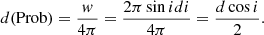
This leads us to assume that it is more likely to observe highly inclined AGN compared to the probability of observing an object at inclination, namely, i0 is ∼ sin i0.
For the case of a single SMBH, we adopted the physical parameters given in Kovačević et al. (2020a), while for the CB-SMBH system, we used the physical parameters given in Songsheng et al. (2019a, see Table 1). For the BLRs, we adopted a disc-like model. The BLR kinematic structures for about two dozens of AGNs, inferred from velocity-resolved RM, indicate a virialised disc, inflow, and outflow BLR geometries (see Lu et al. 2019, and references therein). The latest finding of Lu et al. (2019) indicates that the BLR of Mrk 79, which is sub-Eddington accreting AGN, probably originates from a disc wind launched from the accretion disc. Here, we focus on the most straightforward BLR elliptical disc-like geometry to simulate differential observables.
Returning briefly to the subject of circular binaries (with orbital eccentricities ei = 0, i = 1, 2 and semi-major axes ai, i = 1, 2), we point out the time independence of the relative distance of two SMBH:
 (2)
(2)
where a = a1 + a2. In the circular case, the velocities of SMBHs and their relative velocity are also time-independent. However, in the case of elliptical configurations of clouds in the BLR of SMBH and elliptical CB-SMBH system, the positions and velocities depend on time and osculating orbital elements. Our model accounts for all these parameters, as explained in Kovačević et al. (2020a). We used the parameter ranges in Table 1 to generate different combinations of parameters, and run simulations with 100 clouds in each BLR. The clouds’ orbital positions are uniformly sampled at every time instance tn, n = 1, …, 1000. All simulations were performed at the initial CB-SMBH orbital phase, if not stated otherwise. As an illustrative example, one realisation of elliptical geometrical configuration of CB-SMBH, depicted from the elevated and the side, is shown in Fig. 1. Moreover, Fig. 2 illustrates how our model captures dynamics and, consequently, the distribution of radial velocities of clouds in two BLRs occurring for different clouds’ orbital angular momenta alignments to the CB-SMBH orbital angular momentum, using randomly chosen orbital parameters. We set the radial velocity distributions at clouds positions in each BLR on the same plot for comparison. For each cloud in the disc-like BLR, we determine its combined velocities of orbital motion sampled at 1000 points of its orbit and its angular momenta, taking into account its central SMBH motion. We then project the clouds’ velocity field onto the plane of the observer for a value of i0 to determine the line-of-sight projection of the combined velocity at each position in the inclined disc-like BLRs.
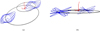 |
Fig. 1. Realisation of a coplanar elliptical CB-SMBH system with clouds in non-coplanar orbits in both BLRs calculated from the model. M1 and M2 show the locations of the SMBHs in a binary system. Blue ellipses are every 20th of the 100 orbits of clouds in each BLR. The SMBH parameters are M1 = 6 ⋅ 107 M⊙, M2 = 4 ⋅ 107 M⊙, A0 = 100, Ω1 = Ω2 = 3° , ω1 = 1° , ω2 = 181° , e1 = e2 = 0.5. Clouds parameters are Ωc1 = Ωc2 = 180° , ωc1 = 2° , ωc2 = 182° , i = ( − 40° ,40° ), e = 0.5, but their orbital planes have different inclinations. The reference plane (BXY) is the plane of the relative orbit of M2 to M1, and the origin of the coordinate system is the barycentre (B) of the CB-SMBH system. (a) Elevation view of the CB-SMBH system. (b) Side view to the YBZ coordinate plane. |
Model parameters and their range of values used in simulations.
The maximum of the V1 and V2 radial velocities of the primary and secondary components in CB-SMBH occur at passaging the ascending node in their true orbits. The epoch of passage through the ascending node corresponds to the instant when radial velocity of the secondary component reaches its maximum (or when the radial velocity of the primary component reaches its minimum). The asymmetry of distributions is a consequence of the asymmetry of elliptical orbital motions of SMBHs and clouds. There is a distinction between radial velocity distributions (see Fig. 2). Specifically, we see the topological difference between velocity fields for aligned (Fig. 2a) and anti-aligned orbital configurations of clouds (Figs. 2b–2d). Consequently, clouds in anti-aligned orbits have inclinations between 90° and 175°. Velocity field for anti-aligned clouds’ orbital momenta shows elongated features that are strained. In all these cases, the clouds’ orbital inclinations are linearly spaced between given boundaries. Velocity fields are the closed surfaces2, preserving topological volume and surface coherency3. We also tested the cases where inclinations are randomly distributed within given ranges, and such velocity fields of the BLRs are not volume-preserving in the topological sense.
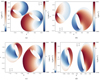 |
Fig. 2. Radial velocity maps of simulated images of the BLRs around the primary and secondary components in CB-SMBH. Abscissas (X) and ordinates (Y) are normalised by 𝒜0 = 100ld. The clouds’ orbital angular momenta alignment with CB-SMBH orbital angular momentum is indicated in legends. (a) A0 = 175ld, i0 = 40°, i = 80°, ld, Ω1 = 300°, Ω2 = 50°, ek = 0.5, k = 1, 2, ω1 = 70°, ω2 = 250°, ic1 = ic2 = 40°, Ωc1 = Ωc2 = 300°, ωc1 = 70°, ωc2 = 250°, ec = 0.5, (b) A0 = 175ld, i0 = 40°, i = 80°, Ω1 = 300°, Ω2 = 50°, ek = 0.5, k = 1, 2, ω1 = 70°, ω2 = 250°, ic1 = (90° ,175° ), ic2 = 40°, Ωc1 = Ωc2 = 300°, ωc1 = 70°, ωc2 = 250°, ec = 0.5, (c) A0 = 175, i0 = 40°, i = 80°, ld, Ω1 = 300°, Ω2 = 50°, ek = 0.5, k = 1, 2, ω1 = 70° ω2 = 250°, ic1 = 40°, ic2 = (90° ,175° ), Ωc1 = Ωc2 = 300°, ωc1 = 60°, ωc2 = 240°, ec = 0.5, (d) A0 = 175, i0 = 40°, i = 80°, ld, Ω1 = 300°, Ω2 = 50°, ek = 0.5, k = 1, 2, ω1 = 70° ω2 = 250°, ic1 = ic2 = (90° ,175° ), ωc1 = ωc2 = 300°, ωc1 = 60°, ωc2 = 240°, ec = 0.5. |
For aligned BLRs, the absolute value of velocity increases toward the outer left- and right-side lobes of disc-like BLRs (regarding the smaller BLR diameter). However, with anti-aligned BLRs, the absolute value of velocity increases toward frontal and backward lobes (oriented in the directions of larger BLR diameters).
As discussed above, the general form of equations for calculation of the brightness distribution of singular SMBH and CB-SMBH systems is the same as in Songsheng et al. (2019a), but the difference is that the input and output variables depend on the time. Replacing the double integral by a summation on the coordinates of clouds and time with single SMBH gives the discrete form of the equations. For the CB-SMBH system, the summation is on the coordinates of clouds in the BLRs, for both SMBHs and time.
2.2. Differential phase
The primary advantage of using differential phase measurements is that their uncertainties are reduced in the case of narrow spectral lines and they are not contaminated by wavelength-independent errors (see Waisberg et al. 2017). We modelled the differential phases from the computed brightness distribution according to the prescription given by Songsheng et al. (2019a) based on the Zernike-van Cittert’s theorem. In particular, from this theorem, we obtain:
 (3)
(3)
where Q(u, λ) is a coherent flux of the object, I(σ, λ) is the intensity of the object emission in the observer direction, transferred the spectral channel of band, δλ, and centred on the wavelength λ; σ = (α, β) is the celestial angular coordinates of an emitting point in the object and 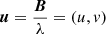 is the interferometry baseline vector. By defining the moments of intensity distribution (see details in Waisberg et al. 2017), we have:
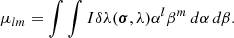 (4)
(4)
We can see that μ00 is total intensity of the object, while the normalised first-order moments give the centroid positions:
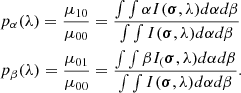 (5)
(5)
Consequently, we have Q(0, λ) = μ00 = Ξ(λ). The emission line (Ξ(λ)) is the zero-order moment of brightness distribution of the object.
Also, from the Zernike-van Cittert’s theorem, the fringe phase is:
 (6)
(6)
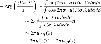
We now consider an unresolved source (u ⋅ σ < 1), for which it is possible to relate vectorial components given in Eq. (6) to the photocentre, pα, pβ (Eq. (5)), of the intensity distribution (see details in Jankov et al. 2001):
 (7)
(7)
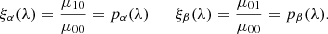
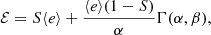
The terms in Eq. (7) are the fringe phase components. They are proportional to the photocentre of intensity distribution and equivalent to the first moment of the intensity distribution. However, the fringe phase can be disrupted by the atmospheric turbulence if only one baseline (two telescopes) is used. This problem can be reduced with the differential phase Δϕ (see e.g. Delaa et al. 2013, and references therein). The differential phase is defined as the difference between the fringe phases obtained in two spectral channels centred on the wavelengths, λ and λr, respectively,
 (8)
(8)
This quantity is relevant for line profiles when accounting for the kinematics of the source and the continuum region is the natural choice as a reference, such that ξ(λr) = 0 (see Domiciano de Souza et al. 2004). Thus, the first vectorial component of differential phase (Eq. (7)) is usually observed and modelled in the literature. We have also followed this approach. It has been shown both empirically (Gravity Collaboration 2018) and theoretically (Songsheng et al. 2019a) that differential interferometry produces a variation of BLR photocentre ξ(λ). It is an unexploited astrophysical parameter in AGN investigation, with an interpretation similar to the BLR spectral lines Ξ(λ). Line profiles reveal a large scale spatial and physical effects of the BLRs. However, with ξ(λ), we can check and add new details to the spectroscopic information to get a complete picture of the object. The information in ξ(λ) is always new because the weights of the contribution of different parts of the object in Ξ(λ) and ξ(λ) are different (Petrov 1989).
All the interferometric data are usually quantitatively interpreted within the frame of a single, self-consistent physical model, which should produce observables. Modern spectro-interferometers can measure the variation of the interferometric phase across an emission line of AGN (Gravity Collaboration 2018). This first measurement of phase displays a simple S-shaped profile comprising a single reversal, arising from the line emission from a circular rotating disc-like BLR. The S form is one of the most common observed differential phase shapes, which we briefly explain here.
Assuming that the source has Gaussian spatial brightness distribution, G(σ, λ), and integrating ξα(λ) (see Eq. (7)) in both directions, β and α, we get that the differential phase shape is:

where erf is an “error function” of sigmoid shape which causes differential phase (Eq. (8)) to be of the S shape. In general, Lachaume (2003) showed that the differential phase can be related to the skewness and diameter of the object flux distribution.
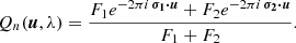
Songsheng et al. (2019a) showed the same reasoning for interferometric observables is valid for the CB-SMBH case. The interferometric model of the CB-SMBH system is a composition of two sources (their BLRs) considered either as point-like or disc-like models with assumed morphologies. Let we denoted the brightness of disc-like BLR components as Ik(σk, λ) and their barycentric positions (σk),k = 1, 2.
The total brightness distribution of such system can be written as
 (9)
(9)
Taking into account Eqs. (3) and (9), the additional and translational property of the Fourier transform, we get the result that the coherent flux is simply:
 (10)
(10)
where F1 and F2 are the fluxes of components. Normalisation gives
 (11)
(11)
We can expand the complex exponential terms in Eq. (11) in a Taylor series:
 (12)
(12)
Taking into account that arctan(x) ∼ x when |x|< 1 and |σk ⋅ u|< 1, k = 1, 2, we can estimate
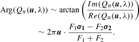 (13)
(13)
If the binary components are on circular orbits, then σ1 = σ and σ2 = σ, where σ is a component barycentric distance. Under this condition, Eq. (13) shows that ξ(λ) signal is proportional to the binary separation σ. However, with CB-SMBH on elliptical orbits, we can expect the ξ(λ) signal to be more complex, especially since spectral lines are compound functions taking the form,  where
where  are composite vector field, representing at each position (
 ) of the mth cloud in the kth BLR, its velocity,
  , given in a CB-SMBH barycentric coordinate system (see Kovačević et al. 2020a).
Moreover, Eqs. (9)–(13) show us that the primary difference between the binary and single models is that the brightness distribution is no longer symmetric, which makes the differential phase become a complex function.
2.3. Observational constrains
The differential phase of the circular CB-SMBH system depends on extrinsic parameters (the inclination of a CB-SMBH system to the observer) and intrinsic parameters (an opening angle of the BLR, SMBH masses and their mutual distance, and the orientation of total angular momentum) as it was shown in Songsheng et al. (2019a). Here, we extend analysis on non-coplanar CB-SMBH system with varying orbital elements and randomly distributed orbital inclinations of the clouds, along with eccentricities and semi-major axes. We choose clouds in randomly inclined orbits as an interesting case based on Wanders et al. (1995) model of C IV emitting region of NGC 5548 with an ensemble of clouds on randomly inclined and spherically distributed orbits around the continuum source. However, this spectral line is observed as blue-shifted with certain blue-asymmetric features, perhaps indicating material outflow. Because of these characteristics, the C IV emitting region is distinctive from those related to Hβ and Paα. Moreover, emission line profiles are indicators of the BLR gas kinematics. None of the functional forms (i.e. Gaussian, Lorentzian, even Power law) is connected directly to the ordered motion of clouds in the BLR. Except for double-peaked profiles, all spectroscopic line shapes are consistent with randomly oriented orbits in a gravitationally bound cloud system (see Netzer 2013). The clouds’ randomly distributed orbital semi-major axes and eccentricities lead to their random position, velocities, and orbital angular momenta. We calculated differential phases for a 100-m baseline with a position angle of 90° to the direction of the semi-major axis of the CB-SMBH system. The differential phases correspond to the emission Paα line, which rest-frame wavelength is λ0 = 1.875 μm for objects at redshift of z ∼ 0.1. These parameters correspond to sources (such as 3C 273), which are red-shifted enough so that the Paα line is in the K band. This band is convenient because the emission is at least two times stronger in Paα than in, for instance, Brγ (Petrov et al. 2012). Moreover, as shown by Landt et al. (2008), the strongest Paschen hydrogen broad emission lines Paα and Paβ are seen to be without strong blends implying good measurement of their widths. The line attenuation by dust is much more reduced in the near-IR lines than in the optical and UV.
3. Results
Here, we present our investigation of the effects of variation of SMBH and the orbital elements of clouds on the amplitude and shape of Paα and the corresponding differential phase. We present the results divided in the domains of observables of the single SMBH and CB-SMBH system. We select representative cases that resemble examples of “real-world” AGN discussed in Sect. 4.1. For each referred AGN, we show the models whose spectrum resembles the observations and the predicted differential phases for that model. The plots from all the combinations of parameters (i.e. the atlas of spectra and differential phases) are shown in the appendix. As expected, the phase signatures occur under specific conditions and their diagnostic potential is clearer for some parameters than for others. The set of models under comparison is composed of those in which one (or all) of the parameters could have different values. For reference, interferometric observables marked with a blue colour in plots were simulated for values at the lower end of the parameters ranges, unless stated otherwise.
3.1. Interferometric signatures of a single SMBH
Here, we explore potential effects, induced by changes in the elliptic orbital parameters of clouds in single BLR, on theinterferometric observables. Before conducting our numerical simulations, we analysed generalised forms of the first-order approximation of the differential phase (Appendix A.1). The predicted deformation of differential phase S-shape is asymmetric, indicating the clouds’ elliptical orbital motion (see Fig. A.1a).
Then, we simulated the Paα lines and corresponding differential phases by considering the orbital dynamics controlled by orbital elements of clouds and different values of the i0 parameter. The curves are given as a function of the wavelength. For a better comparison, the scale of twin x-axis at the top of each plot is presented in radial velocity. First, we adopted that the clouds move on orbits with uniformly distributed inclinations ic = 𝒰(−5° ,5° ) and varying other parameters. The most dramatic evolutions of observables occur when varying either Ωc or ωc between 10° and 180° (see Fig. 3a). For a fixed orbital eccentricity of the clouds, e = 0.5, larger values of Ω and ω cause an increase in the amplitude of the differential phase (see Figs. 3a and 3b). Additionally, these two orbital angle parameters have a more significant influence on the amplitude of the differential phase when eccentricity is smaller as it is shown in Fig. A.1a.
 |
Fig. 3. Evolution of the Paα emission line (upper subplots) and corresponding differential phase (Δϕ, lower subplots) as a function of the wavelength for different values of clouds’ orbital parameters in the different models of single SMBH. Common parameters for all models: (a) and (b) clouds’ orbital inclination ic ∈ [ − 5° ,5° ], clouds’ orbital eccentricity ec = 0.5 and i0 = 45°. (c) Clouds’ orbital inclination ic = 𝒰(−7.5° ,7.5° ), and i0 = 𝒰(10° ,45° ). Varying parameters are given in subcaptions. Here, ℑ = 𝒰(l, r) stands for collection of inclination ranges from 𝒰(−l, l) up to 𝒰(−r, r). For reference, interferometric observables marked with blue colour were modelled for values at the lower end of the parameters ranges. (a) Ωc ∈ 𝒰(10° ,180° ), ωc = 110°, (b) Ωc = 100°, ωc = 𝒰(10° ,180° ), (c) ωc = 200°. |
Furthermore, these simulations capture another characteristic of the spectra: the flat-topped spectra can appear not only for circular motion but also because of the clouds’ elliptical motion (see Figs. 3a and 3b). The shapes of the flat top depend on the angles Ω and ω of the elliptical orbits of clouds. Compared to simulations for small clouds’ orbital eccentricity, we recorded the most notable variations of differential phase shape associated with variation of angle, i0, fixed high orbital eccentricity (e = 0.5) and orbital inclination ic = U(−7.5° ,7.5° ) (see Fig. 3c). The inclination of the observer i0 and the clouds’ orbital inclination affects the slope of the differential phase in a similar way (see Fig. 3c). Here, we also identify a characteristic pattern of alternation in the amplitudes in the left and the right wings of the differential phase because of a variation in the clouds’ orbital pericentre ω (Fig. 3c).
All previous simulations assumed a constant or homogenous distribution for the clouds’ orbital eccentricities. As a valuable study case, the novel simulations for non-homogenous clouds’ orbital elongation have been considered where some interesting effects affecting the differential phase could occur. The detailed distribution of orbits is unknown because clouds have a wide distribution of masses. The elongation of these orbits changes with variation of cloud column densities: high column-density clouds allow for mildly elongated or even circular orbits (the right-skewed eccentricity distribution), but low column density clouds require highly eccentric ones (the left-skewed eccentricity distribution Krause et al. 2011). We can now construct these distributions, reflecting assumptions about skewness based on the clouds’ column density, which will be used in our simulations. Similar to the variable defined for the construction of a skewed random spatial distribution of clouds in BLR models (see Wang et al. 2020a, and references therein), we sampled clouds’ orbital eccentricities from the left-skewed distribution given as:
 (14)
(14)
where S is a random number from an uniform distribution between 0 and 1, ⟨e⟩∼0.8 is the mean value of the random variable, and the parameters of Γ distributions are α = 0.3, β = 1. The random variable in Eq. (14) is a shifted and scaled Γ distribution, thus, we refer to it as Γs. Randomly chosen samples of eccentricities increase steadily with a peak around e ∼ 0.65 − 0.8.
After introducing the left-skewed eccentricity distribution, we outline the right-skewed distribution using Rayleigh distribution ℛ(1), whose probability density function is
 (15)
(15)
In contrast to Γs, random samples of clouds’ orbital eccentricities drawn from ℛ(1) have a peak at e ∼ 0.2 − 0.4. For each of these distributions of eccentricities and ω > 180° of non-coplanar clouds, we observed various broad spectral lines and differential phases (compare Figs. 4a and 4b). Conversely, larger differential phases amplitudes are seen for coplanar orbital configurations of clouds. Clouds’ orbital setups drawn from ℛ yield differential phases with larger amplitudes than more elongated orbital layouts (following shifted Γs distribution). But the effects of observer position, i0, and clouds’ orbital inclinations are the same as in the models with a homogenous distribution of clouds’ eccentricities.
 |
Fig. 4. Same as Fig. 3 but for random samples of clouds’ orbital eccentricities generated from Γs(0.3, 1) and ℛ(1) distributions. Varying parameters are listed in subcaptions and 𝒞 stands for coplanar clouds orbits. (a) i0 = 𝒰(−10° ,45° ), δi0 = 5°, 𝒞, Ωc = 100°, ωc = 270° ,ec ∈ Γs(0.3, 1), (b) i0 = 𝒰(−10° ,45° ), δi0 = 5°, ic = 𝒰(−20° ,20° ), Ωc = 100°, ωc = 270°, ec ∈ ℛ(1). |
Distinctly, for models with clouds with an orbital parameter, ω ≲ 50°, the spectral lines and differential phases are narrower for observer angles smaller than 30° (see Fig. 4b). We found a global geometrical pattern that demonstrates that differential phases are deformed around an invariant point in its right wing for coplanar orbital configurations and different observer positional angles (compare Figs. 4a and 4b). For any value of wavelength that is close enough to the wavelength of the invariant point, the differential phase values are close to the fixed point.
Based on our simulations, the shape of the differential phase obtained from the emission of clouds on elongated orbits is distinctive from circular ones. The typical S-shape signature of a rotating disk is clearly distorted. The peaks are deformed due to the superposition of trigonometric functions of angles controlling the orbital shape arising from the first term in Eq. (A.2) (see also Fig. A.1a, upper plot). In addition, an increasing cloud orbital inclination produces differential phases with smaller amplitudes. These distortions are an illustrative proof of the presence of an asymmetry in the disk. Meilland et al. (2011) showed that for larger baselines, a loss of the simple S shape occurs when stellar environments are dominated by rotation. We summarise the simulation results in Table 2, which shows some general qualitative morphological characteristics of the differential phase for various simulation parameters. Appendix B provides detailed atlas of interferometric observables.
Qualitative summary of simulation parameters effects on the morphology of differential phase (DP) curves for a single SMBH.
3.2. Interferometric signatures of CB-SMBH
Gravity Collaboration (2018) assumes that all clouds have ordered motion when measuring the BLR size and black hole mass of 3C 273. But as pointed out by Stern et al. (2015) and shown for a circular CB-SMBH by Songsheng et al. (2019a), the phase curves could encode the distribution of angular momentum of clouds in the BLR. If GRAVITY provides the angular momentum distribution of clouds, then the clue for BLR formation is expected to be found as well (Wang et al. 2017). In our simulations, all clouds of individual BLRs have their own either clockwise or anti-clockwise rotation. Then, the total angular momentum of the BLR is the vector sum of all the clouds’ orbital angular momenta. The direction of the total BLRs angular momenta (either aligned or counter-aligned with the CB-SMBH system orbital angular momentum) has a strong effect on both interferometric observables as shown in further paragraphs. The orbital angular momentum of CB-SMBH is simply
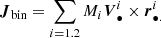
We define the orientation of the cloud orbits (with inclination, ic) to the invariable plane of the CB-SMBH system, which is perpendicular to the total orbital angular momentum, Jbin. In the following, we assume the net angular momenta of BLRs and the orbital angular momentum of CB-SMBH are independent of one another, so there are cases of CB-SMBH with all angular momenta aligned or when one or both of BLR net angular momenta are misaligned. In this section, we consider two sets of results: for aligned and anti-aligned CB-SMBH. Prior to the simulation, we first predict the pattern of differential phases from first order approximation given in Appendix A.2. Prediction surfaces comprise a complex system of two ridges and valleys (see Fig. A.2). Because of such a topology, deformed double S shapes are expected. We present more detailed atlases of CB-SMBH in Appendices C (aligned) and D (anti-aligned).
3.2.1. CB-SMBH system with aligned angular momenta
In these simulations, we focussed on CB-SMBH systems in which all the clouds’ orbital angular momenta in both BLRs are aligned with the CB-SMBH system angular momentum, Jbin ⋅ Jci > 0, i = 1, 2. This condition is equivalent to the condition that clouds in both BLRs have prograde motion, that is, the clouds’ orbital inclinations are ic < 90°. Figure 5a shows some typical interferometry observables for aligned CB-SMBH systems. Even when the spectral lines of both SMBHs are well blended in blue-coloured models in Fig. 5a, corresponding differential phases still show two peaks. Hence, small velocity differences can be measured with differential interferometry (see e.g. Tokovinin 1992). The phases are most sensitive to the asymmetric brightness distribution of the object. Even if the spectra might have differed only slightly in their peculiar aspects, the corresponding differential phases differ clearly. We found that there is a distinction between differential phase “zoo” of single SMBH and CB-SMBH system.
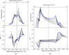 |
Fig. 5. Evolution of the Paα emission line (upper subplots) and the corresponding differential phase (Δϕ, lower subplots) as a function of the wavelength for different values of model parameters for an aligned CB-SMBH system. Orbital elements that are the same for all clouds in both BLR are designated by the subscript, c. Varying parameters are listed in sub-captions; 𝒞 stands for the coplanar CB-SMBH system. (a) i0 = 45° ; ik = 𝒰(90° ,10° ), δik = −10°, Ω1 = 200°, Ω2 = 100°, ωk = 210°, ek = 0.5, k = 1, 2; 𝒥 = 𝒰(5° ,45° ), δ𝒥 = 5°, Ωc = 200°, ωc1 = 150°, ωc2 = 210°, ec = 0.5, (b) i0 = 𝒰(15° ,45° ), δi0 = 5, 𝒞, Ωk = 𝒰(170° ,230° ), δΩk = 20° ωk = 𝒰(270° ,170° ), δωk = −20°, δek = (0.1, 0.5), δek = 0.1, k = 1, 2, ic = 𝒰(−5° ,5° ), Ωc = 𝒰(20° ,160° ), δΩc = 20, ωc = 𝒰(120° ,20° ), δωc = 20°, ec = ek. |
More specifically, the single SMBH “zoo” phases consist of a deformed, but still recognisable, S shape, which indicates the rotational motion of clouds in the BLR. The differential phases of CB-SMBH show a complex structured signal looking as two blended and deformed S-shaped signals. Differential phase variations are related to the orbital motions of clouds and SMBHs. These patterns are asymmetrical about the line centre.
For fixed values of SMBHs and the clouds’ orbital eccentricities, variations in the ranges of the clouds’ orbital inclinations lead to an appearance of ridges in the wings of differential phases (see Fig. 5a). When the orbits of larger SMBH and clouds in its BLR have a smaller angle for the pericentre, the plateaus between peaks of differential phases are less deformed (compare with Fig. 5a). We turn now to the effects in the differential phase for various positions of SMBHs orbits in the orbital plane. Simulations for different combinations of variations of parameters have revealed a wide range of distinct patterns (Fig. 5b). For a simultaneous increase in the observer’s angular position and the orbital inclination of SMBHs and clouds, we observed a broadening of spectral lines and differential phases. Specifically, a plateau between peaks of differential phases flattens and broadens. The more dramatic change of position of differential phase wings is associated with the change of longitude of ascending nodes of SMBHs between 230° −330° (Fig. 5b).
3.2.2. CB-SMBH system with antialigned angular momenta
Next, we look for the effects of retrograde orbital motion of clouds in the BLRs (i.e. ic > 90°) or equivalently with a general class of systems that satisfy the condition, Jbin ⋅ Jci < 0, i = 1, 2. Predicted deformations of the differential phase shows two whirls from the opposite sides of the ridge that are specific to this type of simulation (see the bottom-left plot in Fig. A.2). The shape of whirls vary, depending on the values of the SMBHs and clouds’ longitudes of node and pericentre. We have the appearance of a more or less prominent additional deformation in the form of a depression in the right wing of the surface (the bottom left plot in Fig. A.2). When this deformation is prominent, we can find a specific doubly deformed S shape for the differential phase, as in Fig. D.2.
We consider the case when the CB-SMBH are coplanar while clouds in the BLR of less massive component have anti-aligned angular momenta. The inclinations of orbits of clouds are randomly distributed between 90° and 175° (see Figs. 6a–6c). Much as in considerations of angle distributions of AGN discussed in Sect. 2.1, we can expect a greater frequency of highly inclined cloud orbits. This is a consequence of the form of distribution function for ic, which is given by P(ic)dic = sin icdi. From this one can see that the average ic is about 45°. Moreover, the a priori probability that sin ic > sin 45° is about 87%.
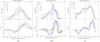 |
Fig. 6. Same as Fig. 5, but for anti-aligned angular momenta of clouds in the BLR of less massive SMBHs. (a) 𝒞, Ω1 = 100°, Ω2 = 300°, ω1 = 250°, ω2 = 70°, ek = 0.5, k = 1, 2; ic1 = rnd(10° ,45° ), ic2 = rnd(90° ,175° ), Ωc = ωc = rnd(0.1° ,359° ,ec = 0.5, (b) 𝒞, Ω1 = 100°, Ω2 = 300° ,ω1 = 250°, ω2 = 70°, ek = 0.5, k = 1, 2; ic1 = rnd(10° ,45° ), ic2 = rnd(90° ,175° ), Ωc1 = 300°, Ωc2 = 100°, ωc1 = 170°, ωc2 = 350°, ec = 0.5, (c) 𝒞, Ω1 = 100°, Ω2 = 300°, ω1 = 250°, ω2 = 70°; ic1 = rnd(10° ,45° ), ic2 = rnd(90° ,175° ), Ωc1 = 300°, Ωc2 = 100° ,ωc1 = 170°, ωc2 = 350°. |
The grid of models presented in Figs. 6a–6c shows that if a more substantial number parameters vary simultaneously, the shapes of differential phases will be more complicated. We can see that the central whirl has deformed wings because of larger ascending node and pericentre (> π/2) of SMBHs and clouds orbits as well for highly inclined orbital motions of clouds (see Figs. 6a–6c). Based on the theory of orbital motion, the variation of orbital nodes is influenced only by perturbations that are perpendicular on the orbital plane. For example, in the case of a spinning SMBH, there may be rocket effect that is orthogonal to the orbital plane (see Redmount & Rees 1989).
Similarly to simulations of non-uniformly elongated clouds’ orbits in the case of single SMBHs (see Sect. 3.1), we consider the same skewed distributions (Γs and Rayleigh ℛ) of clouds’ eccentricities in both BLRs of CB-SMBH system. A general prediction of ℛ distribution effects on the differential phase over the grid of the ascending node and the true anomaly of more massive SMBHs is given in the bottom right plot of Fig. A.2. We observe a rough and unsmoothed surface because of the randomly sampled cloud orbital eccentricities from Rayleigh distribution. Details in Fig. 7a summarise the simulations for different combinations of the Rayleigh distribution for cloud eccentricities and fixed SMBHs, as well as the clouds’ other orbital parameters. We performed simulations separately for the Γs(0.3, 1) distribution of the clouds’ orbital eccentricities. The differential phases are smooth but with subtle differences with regard to the previous case. The central part of differential phase is depressed for coplanar clouds’ motion in both BLRs (see Fig. 7b). For fixed orbital eccentricities of clouds (e = 0.5) around larger SMBHs, irrespective of the coplanarity of their orbital planes, the right wing of differential phase is prominent (Fig. 7b). It seems that subtle distinctions between orbital characteristics of the clouds’ motion could be important and we should avoid the assmption that they are broadly similar.
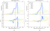 |
Fig. 7. Evolution of the Paα emission line (upper subplots) and corresponding differential phase (Δϕ, lower subplots) as a function of the wavelength for aligned CB-SMBH system when the clouds’ orbital eccentricities are drawn from non-uniform distributions; (a) clouds’ orbital eccentricites are drawn from Rayleigh distribution; (b) clouds’ orbital eccentricities are drawn from scaled and shifted Γs(0.3, 1) distributions. (a) 𝒞, Ωk = 100°, k = 1, 2, ω1 = 110°, ω2 = 290°, ic1 = 𝒰(−5° ,5° ), ic2 = 𝒞, Ωc1 = 200°, Ωc2 = 10°, ωc1 = 150°, ωc2 = 330°, ec1 = ec2 = rndℛ(1), (b) 𝒞, Ωk = 100° ,k = 1, 2, ω1 = 110° ,ω2 = 290°, Ωc1 = 200° ,Ωc2 = 10°, ωc1 = 150°, ωc2 = 330°, ic1 = ic2 = 𝒰(−5° ,5° ), ec1 = 0.5, ec2 = rndΓs(0.3, 1). |
A more extensive atlas of expected interferometric observables probing the elliptical configuration of anti-aligned CB-SMBH systems is given in Appendix D. We summarise the results for the simulation in Table 3, reporting the effects of orbital parameters of the aligned and anti-aligned CB-SMBH system on the differential phase curves. The overall impact on the differential phase is more significant than for the single SMBH case presented in Table 2. We point out the following two effects. Eccentricities of SMBHs orbits, together with SMBH orbital orientation angles, complicate differential phase curves so that even double S-like shapes can appear.
Qualitative summary of simulation parameters effects on the morphology of differential phase (DP) curves for CB-SMBH systems.
4. Discussion
In this work, we probe the detection of interferometric signatures of single SMBH and CB-SMBH systems with elliptical orbital configurations. The differential phase is computed at the wavelength of Paα spectral line. As expected, these signatures in differential phases occur under specific conditions, and their diagnostic potential is more evident for some parameters than for others. To quantify this, we calculated the evolution of the spectral line and differential phase as a function of wavelength and radial velocity for distinct sets of models. Further discussion focusses on three points: anticipated results for specific objects that can be crucial for observers, limitations of the present model in the light of selections of future observational targets, and the information lost due to a random cloud’s motion.
4.1. Anticipated results for future observations
The results of simulations also show interesting qualitative similarities of some synthetic Paα lines with those observed and reported in the literature. The corresponding differential phases might be used as a starting point to predict the interferometric signatures of these specific targets.
Type 1 AGN and single SMBH models expected signatures. With single SMBH models, more or less asymmetric synthetic flat top lines given in Figs. 3a and 3b show similar gradients and shapes with flat top lines reported in the literature by Landt et al. (2014, see their Fig. 2) for IRAS 17500+5046,PDS 456, PG 0026+129, and Mrk 335. These objects are classified as type 1 AGN. Their expected differential phases could be of S-form for single SMBH, but with asymmetric amplitudes and widths of peaks implicating elongated cloud’ orbits. Furthermore, the sharpness of the differential phases peaks became more prominent as Ωc or ωc is increased. The spectral line in Fig. 3c resembles Paα line of SDSS J015530.02-085704.0 (Kim et al. 2010), which is also a type 1 AGN. Here, the anticipated differential phase would be broader as inclination position of the observer is larger, the sharpness of differential phases is more prominent than in the previous case because of larger ωc = 200° and slightly more inclined cloud orbits. Similarly, in the third series of plots of Fig. B.3, the evolution of observables is peculiar. Here, the models keep the orbital eccentricity of clouds constant but vary the inclination angle from i = 5° to i = 40°. We see that amplitude changes of phases are prominent and the position of maxima of phases, which gives an additional tool for interpreting the observations.
The blue lines reported in Figs. B.1a–3b, B.2a, and B.3a show the profiles in the waveform with a more prominent left peak. A comparable pattern was found in PG 0844+349 (Landt et al. 2014, see their Fig. A2). It suggests that predicted differential phases are deformed, when either Ωc or ωc reaches minimal value of ∼10°. The width of the phase increases with increase in clouds’ orbital inclinations. We find that at this wavelength, there is a clear signal in the differential phase for different parameters. In general, single SMBH produces differential phases that are more or less symmetric relative to the core of spectral lines depending on the excitation of eccentricity and parameters controlling the position of clouds orbit.
Type 1 AGN (NLSy1, quasars) and aligned CB-SMBH models expected signatures. Two SMBH and their BLRs induce more rich and complex differential phase patterns. There are many configurations for which the aligned CB-SMBH differs between them and single SMBH. The features of synthetic spectra given in Figs. C.2b and C.2c show a similarity with those found in 3C 390.3 (Landt et al. 2014, see their Fig. A1). This object is well-known as a double-peaked line emitter in the optical band. The double-peaked profiles can be also associated with accretion disc emission (Eracleous & Halpern 1994, 2003; Gezari et al. 2007). However, if the binary model is appropriate for this object, then associated differential phases will have a complex double S-shaped structure. This model reflect the possibility of a non-coplanar CB-SMBH, with highly inclined orbits of clouds in both BLRs. If a single SMBH model with a BLR d of 95 light days is true (see Shapovalova et al. 2010b) a differential signal would be 0.9°. Even that spectral lines of objects can share some characteristics, our model predicts that corresponding differential phases are distinct because of different SMBH and the clouds’ orbital parameters. The optically bright quasar PG 1211+143 (Landt et al. 2014) has a convex Paα shape slightly depressed of the centre, as in our synthetic case present in Fig. C.2a. The predicted differential phase would resemble an asymmetric double S shape, caused by non-coplanarity of the CB-SMBH system and high values for the clouds’ orbital elements Ωc and ωc. Moreover, the high rise spectral line in Fig. 5a is also observed in the spectrum of SDSSJ032213.90+005513.4 (Kim et al. 2010, see their Fig. 1). If the CB-SMBH model is appropriate for this object, then the expected differential phase would be similar in morphology with the previous case but distinct in their details because of different values of Ω2. In addition, asymmetric two horn feature (blue line) found in Fig. C.3b, is also highly consistent with observed line in Mrk 79 (Landt et al. 2008, see their Fig. 13). Anticipated differential phases differ from those seen in previous cases because of large values, 230° < Ω1, Ω2 < 330° , and decreasing ωk, k = 1, 2.
Expected signatures for type 1 AGN (binary black hole candidates, quasars) and anti-aligned CB-SMBH models. Significant changes in differential phase shape for anti-aligned CB-SMBH, are given in Fig. 6a. The spectral line marked as a blue curve in Fig. 6b is akin to the Paα line in SDSSJ015530.02-085704.0 (see Fig. 2 in Kim et al. 2010) and in NGC 7469 (see Fig. 13 in Landt et al. 2008, black line). The expected differential phase for these two objects would have complex double S shape with prominent wings, which is a consequence of anti-aligned orbital angular momenta of clouds in the second BLR and randomised Ωc of clouds orbits in both BLRs. Even double peaks in simulated spectral line merge for larger inclinations of the CB-SMBH system, differential phases preserve more or less deformed double S shape. In the core of NGC 7469, there is a dust torus at a distance of 65–87 light days from the central engine, based on K-band time lags (Suganuma et al. 2006). Thus, expected differential phases could be on the order of 2.17° −3.04°. However, the peculiar spectral line (blue model) in Fig. 6c, with its convex core, resembles the Paα line observed in the binary black hole candidate NGC 4151 (see Fig. 4 in Landt et al. 2008). Here, the expected differential phase has a smaller central part and prominent right wing, caused by anti-aligned orbital angular momenta of clouds in the second BLR. However, Ωc of cloud orbits in both BLRs are not randomised. This object, located at 19 Mpc, is among the nearest galaxies containing an actively growing black hole (Wang et al. 2010). Its proximity and claimed evidence for the first spectroscopically resolved sub-parsec CB-SMBH (Bon et al. 2012) offer one of the best chances also for interferometric studies. Bon et al. (2012) found CB-SMBH to have an eccentric orbit, e ∼ 0.4, with period of 15.2 years, argument of longitude of pericentre, ω ∼ 95°, semi-major axes of (a1 + a2) sin i ∼ 0.002 + 0.008 pc, and masses of components M1 ∼ 3 × 10⁷ M⊙ and M2 ∼ 8.5 × 10⁶ M⊙.
These results imply that the expected signal in the differential phase would be on the order of ∼0.5° , using Eq. (13). CB-SMBH with a small orbital period of the order of 1 yr, as discussed Sect. 4.2, we will be able to observe them at different orbital phases. Figure D.4 shows a set of models depicting interferometric observables calculated at three different CB-SMBH orbital phases Θ(t) = 0, 0.25, 0.5, where  , t is time, τ is the time of the pericentre passage, and P is a binary period. Interferometric observables appeared to be unfavourable in all the cases. However, a careful inspection shows that the interferometric signal varies with orbital phase (i.e. time). These synthetic spectral lines look like those observed in PG 1307+085, PG 0804+761, PG 1211+143, PG 0026+129 (Landt et al. 2014). In summary, we show that using morphological study of differential phases can help us distinguish between models. Although some spectral lines of a single SMBH can be morphologically indistinguishable from those in CB-SMBH, their differential phases differ in various ways and they are likely to serve as an essential tools for CB-SMBH detection.
4.2. Limitation of present model
In our model, we assume that the CB-SMBH orbital period is longer than the dynamical timescale of each BLR, which holds true for separated BLRs. On the other hand, the orbital motion of SMBHs perturb the BLRs, complicating the line profiles and phase curves. For example, periodic flares in the light curves of OJ 287 have been successfully predicted by the model of the secondary SMBH impacting the accretion disc of the primary SMBH, specifically, twice during one orbit (Laine et al. 2020).
We assume the physical parameters of the BLRs emissivity and clouds motion as an unaltered if the orbital period is longer than observational time-baseline. However, if the orbital period of the binary system is of the order of a time baseline of observation, for example, ∼1 year orbital period in the photometric light curve of Mrk 231 (Kovačević et al. 2020b), then these quantities can stray from being invariant.
If the CB-SMBH merged to a later phase, a viable way of overcoming the “final parsec problem” is interaction with a disc surrounding binary (see e.g. Armitage & Natarajan 2005; MacFadyen & Milosavljević 2008). Dissipative torques could align the circumbinary disc plane with the binary orbital plane while a circumbinary disc is rotating in the same sense as the binary (aligned angular momenta). Detailed simulations (see, e.g. Hayasaki et al. 2008) have shown that such triple-disc CB-SMBH systems have tidally deformed BLR discs by the time-varying binary potential because of the orbital eccentricity. Also, Lodato et al. (2009) showed that tidal interaction could transform a circumbinary disc into a decretion regime, which removes angular momentum outward, but with small inward mass transfer. This could prevent the binary separation from being reduced to 10−2 pc. However, it is highly likely that at some point, there will be a retrograde coplanar disc surrounding the binary, would remain in accretion mode. Material from such a disc is gravitationally captured by the binary while its angular momentum decreases. Then, the eccentricity threshold between the circular and non-circular binary system is determined by the surface density distribution of the circumbinary disc (see e.g. Nixon et al. 2011, and references therein). Wang et al. (2020b) explained recent ALMA observation of a counter-rotating disc surrounding the core of NGC 1068 as a binary system with a counter-rotating circumnuclear disc. Also, ALMA observed a gas hole in the core of NGC 1365, NGC 1566, and NGC 1672 (Combes et al. 2019). Similar observations are expected to resolve the signatures of counter-rotating circumnuclear discs.
In addition, we supposed both components in CB-SMBH to share same the non-negligible Eddington ratio (λEdd ∼ 0.1). However, if luminosity variations are much smaller ( λEdd ≲ 0.01), then we can expect a small periodically varying flux component with an amplitude proportional to the black hole mass M• (Haiman et al. 2009):
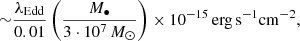
so that object would be too faint for analysis.
Regarding near-infrared observables, they might be detectable if a dusty torus surrounds the binary core. For example, a geometrically thick BLR of a single SMBH in 3C 273 detected by GRAVITY is roughly consistent with dusty torus (Zhang et al. 2019). Thus, the torus inner edge would be irradiated by, and thus mirror, the variable central UV and X-ray sources.
The estimated error of the differential phase (δσϕ), can be obtained from Eq. (13) as a function of errors on the fluxes of both components (δFi, i = 1, 2) and δσi, i = 1, 2 (Eq. (A.4)):
 (16)
(16)
To estimate contribution of terms in the error budget, we first consider that larger component is dominant in CB-SMBH  implying that also
  . Then Eq. (16) is simplified to
 (17)
(17)
Taking into account that  , the angular scale of nearby CB-SBHBs is ∼o(10 μas), with a measured photocentre offset by GRAVITY, and that δσ1 ∼ o(1 μaas) is of the order of precision of GRAVITY photocentre offset measurement of 3C 273, we get

We see that differential phase error is dominated by photocentre offset measurement of the more massive component. However, if  then
then

which is smaller than previous estimate. But we did not consider sources of noise such as the photon noise, the background thermal noise, and the detector readout noise. A crude analysis of Eq. (13) suggests that the cadence of fluxes of both BLRs and photocentre offset measurements are crucial for a well-sampled differential phase curve. Also, we assumed that the object wavelength dependence only comes from the variation of the fluxes of both BLRs. If the object intensity distribution depends on the wavelength in a more sophisticated way, the changes in the phase arise because of effects from the spatial frequency variation and the wavelength-dependency of the object.
4.3. Differential phase loss of information
Interferometric signals decorrelate (become incoherent) due to either instrumental or physical characteristics of an observed object, such as the random motion of clouds in the BLR (see the analysis in Songsheng et al. 2019b). The differential phase curve becomes sensitive to the numbers of the clockwise and counter-clockwise rotating clouds in the BLR, which is essential for GRAVITY measurements of the BLR.
Information loss can be explained by moments introduced in Sect. 2.2. Namely, if the velocity distributions of clockwise and counter-clockwise moving clouds roughly resemble N(0, σ2), then the differential phase as the first-order moment (barycentre) will be zero. In turn, the second-order moment of such distribution will be ∼σ2 ≠ 0. If the disordered motion of clouds in the BLRs comes from turbulence (see Pancoast et al. 2014) then information recovered from the second-order moment would correspond to the parameter of distribution of turbulence velocity field  . Thus higher order moments can contain interferometric information.
5. Conclusions
We used the interferometry-oriented model described here to estimate signatures of the elliptical orbital motion of clouds in the BLR of a single SMBH and elliptical orbital setup of CB-SMBH on spectro-interferometric observables. In addition, we investigate how these observables evolve with a variety of different combinations of orbital and geometrical parameters. Our most important findings and conclusions are summarised below:
-
The differential “zoo” phases for a single SMBH is made up of a deformed, but nonetheless recognisable, S shape, indicating the rotational and asymetrical motion of clouds in BLR. We showed the evolution of differential phase shape, amplitude, and slope with various sets of cloud orbital parameters and observer positions. These maps can be useful for extracting exceptional features of the BLR structure from future high-resolution observations.
-
We found various deviations from the canonical S-shaped phases profile for elliptically configured CB-SMBH systems. There are notable differences between differential “zoo” phases single SMBH and CB-SMBH systems. The differential phases of CB-SMBH appear as two blended and deformed S-shaped signals, asymmetrical along the line centre, whose variabilities depend on the orbital motion of clouds and SMBHs.
-
The shape and amplitude of the phases of CB-SMBH systems depend on presumed orbital characteristics of SMBHs and clouds in their BLRs. Among the many sets of model parameters explored, we found that the signal is sensitive to the position of orbital nodes, inclinations, eccentricities, and arguments of pericentre, along with standardly expected effects related to the geometrical inclination of an observer. The right-skewed distributions of the clouds’ orbital eccentricities cause noise effects in the form of small random fluctuations in the differential phase curve. We found some examples of synthetic spectral lines of a single SMBH, which are indistinguishable from those obtained from the CB-SMBH system, but with differing differential phases. Thus, the differential phases are markers for identifying signals of CB-SMBH.
-
Observationally, the variability of the differential phase is most substantial for lower inclinations for the observer. As much as the central part of the spectral lines is disfigured, the net effect is that the differential phase peaks move away from the line centre. The plateau between differential phase peaks is more prominent. The opposite is valid when there are higher contributions of projected lower velocities in spectral lines. The reversed situation occurs when line peaks are closer together, which is when differential phase peaks move closer to the centre of the line.
-
The velocity distributions for anti-aligned clouds’ orbital momenta in CB-SMBH show elongated features that are strained by the surface positions of clouds. Velocity fields are manifested in the closed surface, preserving their topological volume and spatial coherency. We also tested cases of randomly distributed inclinations, but the velocity fields of such BLRs are not volume-preserving in the topological sense. For the synchronous alignment of the angular momenta of the BLR clouds, the absolute value of clouds’ velocities increases toward the outer side lobes of disc-like BLRs. For anti-aligned BLRs, the absolute values for the velocity increases toward sections that are close to the apocentre and pericentre.
The differential phase precision differs from resolving the object.
Compact and without boundary surface is closed. Notable examples are the sphere and torus. An example of non-closed surfaces is a cylinder.
We use coherence in the sense that levels of velocity intensity do not fluctuate widely.
Acknowledgments
The authors gratefully acknowledge the valuable comments and suggestions of the reviewer, which helped us to improve and clarify our work. A. K. and L. Č. P. are supported by Ministry of Education, Science and Technological development of Republic Serbia through the Astrophysical Spectroscopy of Extragalactic Objects project number 176001. J. M. W. and Y. Y. S. are supported by National Key R&D Program of China through Grant 2016YFA0400701, by NSFC through grants NSFC-11991050, -11873048, and by Grant QYZD-SSW-SLH007 from the Key Research Program of Frontier Sciences, CAS, by the Strategic Priority Research Program of the Chinese Academy of Sciences Grant no. XDB23010400.
References
- Armitage, P. J., & Natarajan, P. 2005, ApJ, 634, 921 [NASA ADS] [CrossRef] [Google Scholar]
- Artymowicz, P., & Lubow, S. H. 1996, ApJ, 467, L77 [NASA ADS] [CrossRef] [Google Scholar]
- Barth, A. J., Pancoast, A., Thorman, S. J., et al. 2011, ApJ, 743, 4 [NASA ADS] [CrossRef] [Google Scholar]
- Barth, A. J., Pancoast, A., Bennert, V. N., et al. 2013, ApJ, 769, 128 [NASA ADS] [CrossRef] [Google Scholar]
- Barth, A. J., Bennert, V. N., Canalizo, G., et al. 2015, ApJS, 217, 26 [NASA ADS] [CrossRef] [Google Scholar]
- Bentz, M. C., Walsh, J. L., Barth, A. J., et al. 2008, ApJ, 689, L21 [NASA ADS] [CrossRef] [Google Scholar]
- Bentz, M. C., Walsh, J. L., Barth, A. J., et al. 2009, ApJ, 705, 199 [NASA ADS] [CrossRef] [Google Scholar]
- Bon, E., Jovanović, P., Marziani, P., et al. 2012, ApJ, 759, 9 [NASA ADS] [CrossRef] [Google Scholar]
- Colpi, M., Mayer, L., & Governato, F. 1999, ApJ, 525, 720 [NASA ADS] [CrossRef] [Google Scholar]
- Combes, F., García-Burillo, S., Audibert, A., et al. 2019, A&A, 623, A79 [NASA ADS] [CrossRef] [EDP Sciences] [Google Scholar]
- Cuadra, J., Armitage, P. J., Alexander, R. D., & Begelman, M. C. 2009, MNRAS, 393, 1423 [Google Scholar]
- Delaa, O., Zorec, J., Domiciano de Souza, D., et al. 2013, A&A, 555, A100 [NASA ADS] [CrossRef] [EDP Sciences] [Google Scholar]
- Denney, K. D., Peterson, B. M., Pogge, R. W., et al. 2009, ApJ, 704, L80 [NASA ADS] [CrossRef] [Google Scholar]
- Domiciano de Souza, A., Zorec, J., Jankov, S., et al. 2004, A&A, 418, 781 [NASA ADS] [CrossRef] [EDP Sciences] [Google Scholar]
- Du, P., Hu, C., Lu, K.-X., et al. 2014, ApJ, 782, 45 [NASA ADS] [CrossRef] [Google Scholar]
- Du, P., Hu, C., Lu, K.-X., et al. 2015, ApJ, 806, 22 [NASA ADS] [CrossRef] [Google Scholar]
- Du, P., Lu, K.-X., Zhang, Z.-X., et al. 2016, ApJ, 825, 126 [NASA ADS] [CrossRef] [Google Scholar]
- Du, P., Zhang, Z.-X., Wang, K., et al. 2018a, ApJ, 856, 6 [NASA ADS] [CrossRef] [Google Scholar]
- Du, P., Brotherton, M. S., Wang, K., et al. 2018b, ApJ, 869, 142 [CrossRef] [Google Scholar]
- Edelson, R., Gelbord, J., Cackett, E., et al. 2019, ApJ, 870, 2 [NASA ADS] [CrossRef] [Google Scholar]
- Elvis, M. 2001, in The Century of Space Science, eds. J. A. Bleeker, J. Geiss, & M. Huber (Kluwer Academiic Publishers), 529 [Google Scholar]
- Eracleous, M., & Halpern, J. P. 1994, ApJS, 90, 1 [NASA ADS] [CrossRef] [Google Scholar]
- Eracleous, M., & Halpern, J. P. 2003, ApJ, 599, 886 [NASA ADS] [CrossRef] [Google Scholar]
- Event Horizon Telescope Collaboration (Akiyama, K., et al.) 2019, ApJ, 875, L1 [NASA ADS] [CrossRef] [Google Scholar]
- Gezari, S., Halpern, J. P., & Eracleous, M. 2007, ApJS, 169, 167 [NASA ADS] [CrossRef] [Google Scholar]
- Gravity Collaboration (Abuter, R., et al.) 2017, A&A, 602, A94 [NASA ADS] [CrossRef] [EDP Sciences] [Google Scholar]
- Gravity Collaboration (Sturm, E., et al.) 2018, Nature, 563, 657 [Google Scholar]
- Grier, C. J., Peterson, B. M., Pogge, R. W., et al. 2012, ApJ, 755, 60 [NASA ADS] [CrossRef] [Google Scholar]
- Grier, C. J., Trump, J. R., Shen, Y., et al. 2017, ApJ, 851, 21 [CrossRef] [Google Scholar]
- Haiman, Z., Kocsis, B., & Menou, K. 2009, ApJ, 700, 1952 [NASA ADS] [CrossRef] [Google Scholar]
- Hayasaki, K., Mineshige, S., & Ho, L. C. 2008, ApJ, 682, 1134 [NASA ADS] [CrossRef] [Google Scholar]
- Hopkins, P. F., Hernquist, L., Cox, T. J., et al. 2006, ApJS, 163, 1 [Google Scholar]
- Ilić, D., Oknyansky, V., Popović, L., et al. 2020, A&A, 638, A13 [CrossRef] [EDP Sciences] [Google Scholar]
- Jaffe, W., Meisenheimer, K., Röttgering, H. J. A., et al. 2004, Nature, 429, 47 [NASA ADS] [CrossRef] [PubMed] [Google Scholar]
- Jankov, S., Vakili, F., Domiciano de Souza, A. Jr, & Janot-Pacheco, E. 2001, A&A, 377, 721 [NASA ADS] [CrossRef] [EDP Sciences] [Google Scholar]
- Kaspi, S., Smith, P. S., Netzer, H., et al. 2000, ApJ, 533, 631 [NASA ADS] [CrossRef] [Google Scholar]
- Kaspi, S., Brandt, W. N., Maoz, D., et al. 2007, ApJ, 659, 997 [NASA ADS] [CrossRef] [Google Scholar]
- Kim, D., Im, M., & Kim, M. 2010, ApJ, 724, 386 [NASA ADS] [CrossRef] [Google Scholar]
- Kishimoto, M., Hönig, S. F., Antonucci, R., et al. 2009, A&A, 507, L57 [NASA ADS] [CrossRef] [EDP Sciences] [Google Scholar]
- Klioner, S. 2003, ApJ, 125, 1580 [NASA ADS] [CrossRef] [Google Scholar]
- Kovačević, A., Wang, J.-M., & Popović, Č. L. 2020a, A&A, 635, A19 [CrossRef] [EDP Sciences] [Google Scholar]
- Kovačević, A. B., Yi, T., Dai, X., et al. 2020b, MNRAS, 494, 4069 [CrossRef] [Google Scholar]
- Krause, M., Burkert, A., & Schartmann, M. 2011, MNRAS, 411, 550 [CrossRef] [Google Scholar]
- Lachaume, R. 2003, A&A, 400, 795 [NASA ADS] [CrossRef] [EDP Sciences] [Google Scholar]
- Laine, S., Dey, L., Valtonen, M., et al. 2020, ApJ, 894, L1 [CrossRef] [Google Scholar]
- Landt, H., Bentz, M. C., Ward, M. J., et al. 2008, ApJS, 174, 282 [NASA ADS] [CrossRef] [Google Scholar]
- Landt, H., Ward, M. J., Elvis, M., & Karovska, M. 2014, MNRAS, 439, 1051 [NASA ADS] [CrossRef] [Google Scholar]
- Lodato, G., Nayakshin, S., King, A. R., & Pringle, J. E. 2009, MNRAS, 398, 1392 [NASA ADS] [CrossRef] [Google Scholar]
- Lu, K.-X., Bai, J.-M., Zhang, Z.-X., et al. 2019, ApJ, 887, 13 [CrossRef] [Google Scholar]
- MacFadyen, A. I., & Milosavljević, M. 2008, ApJ, 672, 83 [Google Scholar]
- Mayer, L., Kazantzidis, S., Madau, P., et al. 2007, Science, 316, 1874 [NASA ADS] [CrossRef] [PubMed] [Google Scholar]
- Meilland, A., Delaa, O., Stee, Ph., et al. 2011, A&A, 532, A80 [NASA ADS] [CrossRef] [EDP Sciences] [Google Scholar]
- Netzer, H. 2013, The Physics and Evolution of Active Galactic Nuclei (Cambridge University Press) [CrossRef] [Google Scholar]
- Nixon, C. J., Cossins, P. J., King, A. R., & Pringle, J. E. 2011, MNRAS, 412, 1591 [NASA ADS] [CrossRef] [Google Scholar]
- Pancoast, A., Brewer, B. J., & Treu, T. 2014, MNRAS, 445, 3055 [NASA ADS] [CrossRef] [Google Scholar]
- Pancoast, A., Skielboe, A., Pei, L., et al. 2019, ApJ, 871, 108 [CrossRef] [Google Scholar]
- Peters, P. C., & Mathews, J. 1963, Phys. Rev., 131, 435 [NASA ADS] [CrossRef] [Google Scholar]
- Peterson, B. M., Wanders, I., Bertram, R., et al. 1998, ApJ, 501, 82 [NASA ADS] [CrossRef] [Google Scholar]
- Peterson, B. M., Berlind, P., Bertram, R., et al. 2002, ApJ, 581, 197 [NASA ADS] [CrossRef] [Google Scholar]
- Peterson, B. M., Ferrarese, L., Gilbert, K. M., et al. 2004, ApJ, 613, 682 [Google Scholar]
- Petrov, R. G. 1989, in Diffraction-Limited Imaging with Very Large Telescopes, Proceedings of the NATO Advanced Study Institute, held in Cargese, September 13–23, 1988, eds. D. M. Alloin, & J. M. Mariotti (Dordrecht: Kluwer), NATO ASI Ser. C, 274, 249 [Google Scholar]
- Petrov, R. G., Malbet, F., Weigelt, G., et al. 2007, A&A, 464, 1 [NASA ADS] [CrossRef] [EDP Sciences] [Google Scholar]
- Petrov, R. G., Millour, F., Lagarde, S., et al. 2012, in Optical and Infrared Interferometry III, eds. F. Delplancke, J. K. Rajagopal, F. Malbet, et al., Proc. SPIE, 8445, 84450W–1 [Google Scholar]
- Popović, L. Č., Shapovalova, A. I., Ilić, D., et al. 2011, A&A, 528, A130 [NASA ADS] [CrossRef] [EDP Sciences] [Google Scholar]
- Popović, L. Č., Shapovalova, A. I., Ilić, D., et al. 2014, A&A, 572, A66 [NASA ADS] [CrossRef] [EDP Sciences] [Google Scholar]
- Redmount, I. H., & Rees, M. J. 1989, Comm. Astrophys., 14, 165 [Google Scholar]
- Roedig, C., Dotti, M., Sesana, A., Cuadra, J., & Colpi, M. 2011, MNRAS, 415, 3033 [NASA ADS] [CrossRef] [Google Scholar]
- Safarzadeh, M., Loeb, A., & Reid, M. 2019, MNRAS, 488, L90 [CrossRef] [Google Scholar]
- Sesana, A. 2010, ApJ, 719, 851 [NASA ADS] [CrossRef] [Google Scholar]
- Shapovalova, A. I., Burenkov, A. N., Carrasco, L., et al. 2001, A&A, 376, 775 [NASA ADS] [CrossRef] [EDP Sciences] [Google Scholar]
- Shapovalova, A. I., Doroshenko, V. T., Bochkarev, N. G., et al. 2004, A&A, 422, 92 [NASA ADS] [CrossRef] [EDP Sciences] [Google Scholar]
- Shapovalova, A. I., Popović, L. Č., Collin, S., et al. 2008, A&A, 486, 99 [NASA ADS] [CrossRef] [EDP Sciences] [Google Scholar]
- Shapovalova, A. I., Popović, L. Č., Burenkov, A. N., et al. 2010a, A&A, 509, A106 [NASA ADS] [CrossRef] [EDP Sciences] [Google Scholar]
- Shapovalova, A. I., Popović, L. Č., Burenkov, A. N., et al. 2010b, A&A, 517, A42 [NASA ADS] [CrossRef] [EDP Sciences] [Google Scholar]
- Shapovalova, A. I., Popović, L. Č., Burenkov, A. N., et al. 2012, ApJS, 202, 10 [NASA ADS] [CrossRef] [Google Scholar]
- Shapovalova, A. I., Popović, L. Č., Burenkov, A. N., et al. 2013, A&A, 559, A10 [NASA ADS] [CrossRef] [EDP Sciences] [Google Scholar]
- Shapovalova, A. I., Popović, L., Chavushyan, V. H., et al. 2016, ApJS, 222, 25 [NASA ADS] [CrossRef] [Google Scholar]
- Shapovalova, A. I., Popović, L., Chavushyan, V. H., et al. 2017, MNRAS, 466, 4759 [Google Scholar]
- Shapovalova, A. I., Popović, L. Č., Afanasiev, V. L., et al. 2019, MNRAS, 485, 4790 [NASA ADS] [CrossRef] [Google Scholar]
- Shen, Y., Horne, K., Grier, C. J., Peterson, B. M., Denney, K. D., et al. 2016, ApJ, 818, 30 [NASA ADS] [CrossRef] [Google Scholar]
- Songsheng, Y. Y., Wang, J.-M., Li, Y.-R., & Du, P. 2019a, ApJ, 881, 140 [CrossRef] [Google Scholar]
- Songsheng, Y. Y., Wang, J.-M., & Li, Y.-R. 2019b, ApJ, 883, 184 [CrossRef] [Google Scholar]
- Songsheng, Y.-Y., Xiao, M., Wang, J.-M., & Ho, L. C. 2020, ApJS, 247, 3 [NASA ADS] [CrossRef] [Google Scholar]
- Stern, J., Hennawi, J. F., & Pott, J.-U. 2015, ApJ, 804, 57 [NASA ADS] [CrossRef] [Google Scholar]
- Suganuma, M., Yoshii, Y., Kobayashi, Y., et al. 2006, ApJ, 639, 46 [NASA ADS] [CrossRef] [Google Scholar]
- Swain, M. R. 2004, in Proceedings of SPIE, ed. W. A. Traub (Bellingham, WA: The International Society for Optical Engineering), 5491, 2004, 1 [Google Scholar]
- Tokovinin, A. 1992, in Proceedings of ESO Conference on High-Resolution Imaging by Interferometry II. Ground-Based Interferometry at Visible and Infrared Wavelengths, Garching bei Munchen, Germany, October 15–18, 1991, eds. J. M. Beckers, & F. Merkle (Garching bei Munchen, Germany: European Southern Observatory), 425 [Google Scholar]
- Vannier, M., Petrov, R. G., Lopez, B., & Millour, F. 2006, MNRAS, 367, 825 [NASA ADS] [CrossRef] [Google Scholar]
- Waisberg, I., Dexter, J., Pfuhl, O., et al. 2017, ApJ, 844, 72 [NASA ADS] [CrossRef] [Google Scholar]
- Wanders, I., Goad, M. R., Korista, K. T., et al. 1995, ApJ, 453, L87 [NASA ADS] [CrossRef] [Google Scholar]
- Wang, J., Fabbiano, G., Risaliti, G., et al. 2010, ApJ, 719, L208 [NASA ADS] [CrossRef] [Google Scholar]
- Wang, J. M., Du, P., Hu, C., et al. 2014, ApJ, 793, 108 [NASA ADS] [CrossRef] [Google Scholar]
- Wang, J.-M., Du, P., Brotherton, M. S., et al. 2017, NatAs, 1, 775 [Google Scholar]
- Wang, J., Xu, D. W., & Wei, J. Y. 2018a, ApJ, 858, 49 [NASA ADS] [CrossRef] [Google Scholar]
- Wang, J.-M., Songsheng, Y.-Y., Li, Y.-R., & Zhe, Y. 2018b, ApJ, 862, 171 [NASA ADS] [CrossRef] [Google Scholar]
- Wang, J.-M., Songsheng, Y.-Y., Li, Y.-R., Du, P., & Zhang, Z.-X. 2020a, Nat. Astron., 4, 517 [CrossRef] [Google Scholar]
- Wang, J.-M., Songsheng, Y.-Y., Li, Y.-R., Du, P., & Zhe, Y. 2020b, MNRAS, 497, 1020 [CrossRef] [Google Scholar]
- Weigelt, G., Hofmann, K.-H., Kishimoto, M., et al. 2012, A&A, 541, L9 [NASA ADS] [CrossRef] [EDP Sciences] [Google Scholar]
- Zhang, Z. X., Du, P., Smith, P. S., et al. 2019, ApJ, 876, 14 [CrossRef] [Google Scholar]
Appendix A: General inferences about differential phase based on a first-order approximation
A.1. Single SMBH
First, we infer some generic patterns about differential phase shape to assess more specific results of numerical simulations. We recall that spectral line of the source can be approximated as a function of the form  where
where  are composite vector fields of the kth cloud’ position and velocity, given in SMBH centred coordinate system (see Kovačević et al. 2020a) Considering a single-source model, a first-order approximation of ξ(λ) based on Eq. (11) is:
 (A.1)
(A.1)
When u ⋅ σ gets smaller below the resolution limit, the phase tends to a linear expression as it is given by the third term in Eq. (A.1) (Vannier et al. 2006). Thus, the shape of the differential phase is defined by the projected vectorial field of positions of clouds. For non-resolved sources, the term 2πu ⋅ σ never reaches the value of  and the maximum value of phase occrus when u ⋅ σ is largest. Thus, the elements of clouds elliptical orbit appear in the scalar product:
![Mathematical equation: $$ \begin{aligned}&\boldsymbol{u}\cdot \boldsymbol{\sigma } = u \frac{r_{c}}{d}\left[\cos \Omega _{c} \cos (\omega _{c} +f_{c})-\sin \Omega _{c} \sin (\omega _{c}+f_{c})\cos i_{c}\right] \nonumber \\&\qquad \ \ +v \frac{ r_{c}}{d} \left[\sin \Omega _{c} \cos (\omega _{c} +f_{c})+\cos \Omega _{c} \sin (\omega _{c}+f_{c})\cos i_{c}\right], \end{aligned} $$](/articles/aa/full_html/2020/12/aa38733-20/aa38733-20-eq61.gif) (A.2)
(A.2)
where d is the distance between the observer and the SMBH. The intensity of the radius vector of clouds’ orbit is
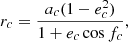 (A.3)
(A.3)
where the true anomaly of fc is computed as outlined in Kovačević et al. (2020a). Since we assume that the interferometric baseline is perpendicular to the rotation axis (PA = 90°, see more in Songsheng et al. 2019a, and references therein) then our calculations will not show second terms containing a v-coordinate of the vector, u.
Having defined quantity u ⋅ σ in terms of the clouds’ orbital parameters and angular position of interferometric baseline, we then move on to discuss the interactive effects of the clouds’ orbital elements on the value of the first term in Eq. (A.2) using surface plots. In Fig. A.1a, we present the surface mesh for ω = π/3, i = π/3, e = 0.5, a = 15 ld which is plotted over Ω - f grid. The surface is smooth with regions of local extrema and a central peak, but some slopes are skewed.
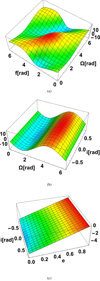 |
Fig. A.1. Interactive effects of clouds’ orbital elements on the values of the first parameter in Eq. (A.2) present as the surface mesh. (a) X axis shows the clouds’ ascending node Ω, the y axis shows the true anomaly (f), z axis shows values of the calculated parameter for fixed elements ω = π/3, i = π/3, e = 0.5, a = 15 ld. (b) X axis shows the clouds’ orbital inclination and fixed elements are ω = 4.66 rad, f = 3.38 rad, e = 0.19. (c) X axis shows the eccentricity and fixed elements are ω = 11π/18, Ω = 10π/18, f = 0 rad. |
An increase in the surface’s amplitude results from an increase of the eccentricity of clouds’ orbits. This is evident even for smaller clouds’ orbital inclinations (see Fig. A.1c). An increasing clouds’ orbital inclination causes peak slopes to decrease in the diagonal direction (see the red region in Fig. A.1a). Deformed side intersections have an S-like shape. The effects of fixed parameters ω = 4.66 rad, f = 3.38 rad, e = 0.19 resemble a wavelike, or hilly, structure with S side profile (see Fig. A.1b), but with deformed peaks (see red and blue regions).
It is useful, for presenting results that follow, to get an analytical estimate of the first term in Eq. (A.2) for some specific values of model parameters. When clouds’ orbital inclinations are ∼0°, the term becomes  . If Ω ∼ 0°, the term turns into
  . At the initial time (i.e. f = 0), the term becomes
  . Thus, its amplitude depends on values of Ω and ω, and having the largest values for smaller eccentricity (see Fig. A.1c).
We explore the analytic forms under degenerate cases, when some orbital parameters are not defined. The simplest case is an inclined circular orbit for which we cannot define f and ω. Then, the so-called argument of latitude η is used and the first term becomes:
For circular orbits with zero inclination, the argument of latitude η is also undefined since the line of nodes is undetermined. Thus, the true longitude L can be used instead, so the first term asymptotically behaves as  .
.
A.2. CB-SMBH
Then we take a brief look at Eq. (13) and describe some general effects of orbital elements of clouds in both BLR in a CB-SMBH system on characteristics of the composite differential phase of. For simplicity, we omit fluxes Fk, k = 1, 2 in the following derivation:
 (A.4)
(A.4)
where σk, k = 1, 2 are vectors of relative positions of clouds around kth SMBH in the barycentric frame. The vector σk equals to the difference between the SMBH barycentric position, r•k, and cloud barycentric positions,  for k = 1, 2. Similar to the case of a single SMBH, we calculate the surface mesh of approximate values of the composite differential phase (see Fig. A.2) using Eq. (A.4). We plot it on a grid defined by orbital ascending node and the true anomaly of the more massive SMBH. To test the differential phase sensitivity to parameters, we varied the parameter values within their ranges, as reported in Table A.1.
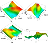 |
Fig. A.2. Surface mesh of the values of the first parameter in Eq. (13) over a grid of orbital elements of larger SMBH. The ascending node Ω1 and true anomaly f1 are given in the XY coordinate plane, and values of the calculated parameter are given on the Z-axis. Upper left plot: Case I – parameters are listed in Table A.1a. Upper right plot: Case II – parameters are listed in Table A.1b. Bottom left: Case III – parameters are listed in Table A.1c. Bottom right: Case IV – parameters are listed in Table A.1d. |
Parameter sets used in testing the differential phase sensitivity for CB-SMBH based on Eq. (A.4).
The calculated surface consists of two ridges and two valleys. The appearance of a complex system of ridges depends on eccentricities and ascending nodes of both SMBHs. If eccentricities of both SMBHs are smaller than 0.5, the second ridge would disappear. Moreover, orbital ascending nodes and angles of pericentre of both SMBHs affect the position and slope of ridges and valleys. The inclinations of SMBH orbits control the slopes of ridges, and the larger inclination values decrease slopes. The effects of clouds and SMBHs orbital elements are similar, but former effects are smaller. The system of ridges and valleys cause complicated differential phase shapes similar to the surface side intersections (upper and bottom left plots of Fig. A.2).
Appendix B: Atlas of interferometric observables for single SMBH
We present three atlases of observables, assuming non-randomised motion. In the first series, shown in Fig. B.1, the clouds’ orbital inclinations have uniform distribution ic = 𝒰(−5° ,5° ). The evolutions of observables depicted in Fig. B.1a are less dramatic then in Figs. 3a and 3b. Variation of i0 shapes the evolution of both observables with largest effects seen when ωc = 270° (see Figs. B.1b–B.1d). The left peak of the spectral line is more prominent when Ωc, ωc ≤ 180° and ec > 0.3, but the right peak dominates when ωc = 270°. These two orbital parameters have a more significant influence on the amplitude of differential phase when eccentricity is smaller (Figs. B.1b–B.1c). Notable net effects of both orbital shape angles are found when they have simultaneously larger values (compare Figs. B.1c and B.1d to B.1b).
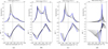 |
Fig. B.1. Evolution of the Paα emission line (upper subplots) and corresponding differential phase (Δϕ, lower subplots) as a function of the wavelength and radial velocity for different values of the clouds’ orbital parameters in the model of single SMBH. Model parameters are given in the sub-captions. (a) Ωc ∈ 𝒰(10° ,90° ), ωc = 110°, ic ∈ 𝒰(−5° ,5° ), ec = 0.5, i0 = 45°, (b) ic = 𝒰(−5° ,5° ), Ωc = 100°, ωc = 10°, i0 = 45°, ec = 𝒰(0.1, 0.5), (c) ic = 𝒰(−5° ,5° ), Ωc = 100°, ωc = 110°, i0 = 45°, ec = 𝒰(0.1, 0.5), (d) ic = 𝒰(−5° ,5° ), Ωc = 100°, ec = 0.5, ωc = 270°, i0 = 𝒰(10° ,45° ). |
In the second series of plots (see Fig. B.2), simulations show the flat-topped spectra. An increase in the clouds’ orbital inclination results in a decrease in the slope between two peaks of the differential phase (Figs. B.2a–B.2b). The inclination of the observer i0 affects the slope of the differential phase similarly to that of the clouds’ orbital inclination (see Fig. B.2c). Also, an alternation of the amplitudes in the left and the right wing of differential phase occurs because of variation of the clouds’ orbital pericentre ω. Smaller ω causes larger amplitudes in the right wing of differential phases, while larger ω has the opposite effect (see Figs. B.1 and B.3). Also, Fig. B.3c shows gradual evolution of the asymmetry of differential phases amplitudes for variation of the angle of pericentre. The slight variation of the slope between the differential phase peaks occurs when ω ∼ π. Finally, we compare the evolution of the spectral lines and differential phases for the two non-uniform clouds’ orbital eccentricity distributions (see Fig. B.4). When ω ≲ 50° and i0 < 30° the spectral lines and differential phases are narrower. For coplanar cases, differential phases’ deformation occurs regarding an invariant point in its right wing (compare Figs. B.4b, B.4d, B.4f versus Figs. B.4e and B.4c).
 |
Fig. B.2. Same as Fig. B.1 but for fixed values of clouds’ orbital eccentricities, ec = 0.5, and angular position of observer, i0 = 45°. (a), (b) Ωc = 100°. The range of the clouds’ orbital inclinations for each model is from 𝒰(−5°, 5°) to 𝒰(−20°, 20°). (a) ωc = 10, (b) ωc = 110°, (c) Ω = 210°, ωc = 10°, ec = 0.5, ic = 𝒰(−7.5° ,7.5° ), i0 = 𝒰(10° ,45° ). |
 |
Fig. B.3. Same as Fig. B.1 but for the range of clouds’ orbital inclinations from 𝒰(−5°, 5°) to 𝒰(−20°, 20°), with fixed values of the clouds’ orbital eccentricities, ec = 0.5, and i0 = 15°. The rest of the parameters are given in the sub-captions of the plots. (a) ωc = 10°, (b) ωc = 110°, (c) ic = 𝒰(−40° ,40° ), i0 = 45°, ωc = (10° ,180° ). |
 |
Fig. B.4. Same as Fig. B.1 but for random samples of clouds’ orbital eccentricities generated from Γs(0.3, 1) and ℛ(1) distributions. Varying parameters are listed in sub-captions. 𝒞 stands for coplanar clouds orbits. (a) i0 = 𝒰(−10° ,45° ), δi0 = 5°, ic = 𝒰(−20° ,20° ), Ωc = 100°, Ωc = 270°, ec ∈ Γs(0.3, 1), (b) i0 = 𝒰(−10° ,45° ), δi0 = 5°, 𝒞, Ωc = 100°, ωc = 270°, ec ∈ ℛ(1), (c) i0 = 𝒰(−10° ,45° ), δi0 = 5°, ic = 𝒰(−10° ,10° ), Ωc = 100°, ωc = 10°, ec ∈ ℛ(1), (d) i0 = 𝒰(−10° ,45° ), δi0 = 5°, 𝒞, Ωc = 100°, ωc = 10°, ec ∈ Γs(0.3, 1), (e) i0 = 𝒰(−10° ,45° ), δi0 = 5° ,ic = ( − 7.5° ,7.5° ), Ωc = 100°, ωc = 10°, ec ∈ Γs(0.3, 1), (f) i0 = 𝒰(−10° ,45° ), δi0 = 5°, 𝒞, Ωc = 100° ,ωc = 10°, ec ∈ ℛ(1). |
Appendix C: Atlas of interferometric observables for aligned CB-SMBH
The typical differential interferometry data for CB-SMBH systems are presented in Figs. C.1–C.3 with partially resolved multi-peaks spectra. Even when the spectral lines of both SMBHs are well blended as in blue-coloured models in Figs. C.1d and C.2d, their differential phases have two peaks. The profiles and differential phases in Figs. C.2c and C.3d are less dependent on angles Ω and ω of SMBHs and clouds. In this case, eccentricity is the same for SMBHs and clouds in the BLRs. These and other examples illustrate that information from the observables suffices to remove the ambiguities between the orbital elements (see e.g. Figs. C.1b and C.1c).
 |
Fig. C.1. Evolution of the Paα emission line (upper subplots) and corresponding differential phase (Δϕ, lower subplots) as a function of the wavelength radial velocity for different models of aligned CB-SMBH system. Common clouds’ orbital elements are designed by subscript c. 𝒞 stands for the coplanar CB-SMBH system. ℑ = 𝒰(l, r) stands for inclination ranges from 𝒰(−l, l) up to 𝒰(−r, r). (a) i0 = 45° ;𝒞, Ωk = 100°, ωk = 110°, ek = 𝒰(0.05, 0.1 − 0.4, 0.45), k = 1, 2, δek = 0.1; ic = 𝒰(−5° ,5° ), Ωc = 10°, ωc = 180°, |

 |
Fig. C.2. Same as Fig. C.1 but for different SMBHs and clouds’ orbital parameters. Plot (c): rnd stands for randomly chosen samples of orbital elements. ℑ = 𝒰(l, r) stands for inclination ranges from 𝒰(−l, l) up to 𝒰(−r, r). (a) i0 = 45° ;ik = 𝒰(10° ,90° ), δik = 10°, Ωk = 200°, ωk = 210°, ek = 0.5, k = 1, 2; 𝒥 = 𝒰(5° ,45° ), δ𝒥 = 5°, Ωc = 200°, ωc1 = 290° ,ωc2 = 210°, ec = 0.5, (b) i0 = 45° ;ik = 𝒰(90° ,10° ), δik = −10°, Ωk = 200°, ωk = 210°, ek = 0.5, k = 1, 2; 𝒥 = 𝒰(5° ,45° ), δ𝒥 = 5°, Ωc = 200°, ωc1 = 290°, ωc2 = 210° ,ec = 0 : 5, (c) i0 = 45° ;ik = 𝒰(10° ,90° ), δik = −10°, Ω1 = 200°, Ω2 = 100°, ωk = 210°, ek = 0.5, k = 1, 2; Ωc = 200° ,ωc1 = 150°, ωc2 = 210° ,ic1 = rnd(5° ,45° ), ic1 = (5° ,45° ), ec = 0.5, (d) i0 = 45° ;ik = 𝒰(90° ,10° ), δik = −10° ,Ωk = 5°, ω1 = 5°, ω2 = 180°, ek = 0.5, k = 1, 2; 𝒥 = 𝒰(5° ,45° ), δ𝒥 = 5°, ec = 0.5, Ωc = 100°, ωc1 = 5°, ωc2 = 180°, (e) i0 = 45° ;ik = 𝒰(5° ,45° ), δik = 10°, Ωk = 5°, ω1 = 5°, ω2 = 180° ,ek = 0.5, k = 1, 2; 𝒥 = 𝒰(5° ,45° ), δ𝒥 = 5°, Ωc = 100°, ωc1 = 5°, ωc2 = 180°, ec = 0.5. |
 |
Fig. C.3. Same as Fig. C.1 but for different SMBHs and clouds’ orbital parameters. (a) i0 = 𝒰(10° ,45° ), δi0 = 5° ;ik = (10° ,90° ), δik = −10°, Ωk = 5°, ω1 = 5°, ω2 = 180°, ek = 0.5, k = 1, 2; 𝒥 = 𝒰(10° ,45° ), δ𝒥 = 5°, Ωc = 100° ,ωc1 = 5°, ωc2 = 180° ,ec = 0.5, (b) i0 = 𝒰(15° ,45° ), δi0 = 5° ;ik = 𝒰(80° ,20° ), δik = −10° ,Ωk = 𝒰(230° ,330° ), δΩk = 20°, ωk = 𝒰(270° ,170° ), δωk = 20° ,ek = 0.5, k = 1, 2; 𝒥 = 𝒰(5° ,45° ), δ𝒥 = 5°, Ωc = 𝒰(80° ,180° ), δΩc = 20, ωc = 𝒰(120° ,20° ), δωc = 20° ,ec = 0.5, (c) i0 = 45° ;ik = 𝒰(10° ,90° ), δik = 10° ,Ωk = 5°, ω1 = 5° , ω2 = 180°, ek = 0.2, k = 1, 2;𝒥 = 𝒰(5° ,45° ), δ𝒥 = 5°, Ωc = 200° ,ωc1 = 290°, ωc2 = 210° ,ec = 0.2, (d) i0 = 45° ;ik = 5°, Ωk = 𝒰(20° ,180° ), δΩk = 20°, ωk = 𝒰(180° ,20° ), δωk = −20°, ek = 0.5, k = 1, 2; ic = 5° ,Ωc = Ωk, ωc1 = ωk, ec = 0.5, (e) i0 = 𝒰(20° ,45° ), δi0 = 5° ;ik = 10°, Ωk = 𝒰(230° ,330° ), δΩk = 20°, ωk = 𝒰(270° ,190° ), δωk = −20°, ek = 0.5, k = 1, 2; ic = 5°, Ωc = 𝒰(80° ,180° ), δΩk = 20° ,ωc1 = 𝒰(120° ,20° ), δωk = −20° ,ec = 0.5. |
For a fixed observer position, i0, and with increasing SMBHs orbital eccentricity, the amplitude of differential phase decreasing, but with distorted left and right wings (see Figs. C.1a and C.1e). Also, large angles of pericentre of clouds’ orbits in both BLRs ωc > π/2 deform core of the differential phase below 0 value. However, an increasing of the angular position of the observer i0 and SMBH’s orbital inclination decreases the slopes of the differential phase (see Figs. C.1d–C.1e). In contrast, Figure C.1f shows obscured effects of clouds’ orbital inclination for the fixed observer angle and eccentricities of both SMBHs. For fixed eccentricities of SMBHs and clouds’ orbits, different ranges of clouds’ orbital inclinations influence appearance of ridges in the wings of differential phases (compare Figs. C.2a–C.2c, and C.2d). For the smaller angle of a pericentre of larger SMBH and clouds in its BLR, plateaus between peaks of differential phases are less deformed (see Figs. C.2d–C.2e).
If both SMBHs orbits have small ascending nodes, but the larger SMBH orbit has a smaller angle of pericentre, then varying SMBHs and clouds’ orbital inclinations affects the amplitude of differential phase wings (Fig. C.3c).
Appendix D: Atlas of interferometric observables for anti-aligned CB-SMBH
We first look at the case of coplanar CB-SMBH, clouds of less massive SMBH have anti-aligned angular momenta, and the inclinations of orbits of clouds are linearly spaced between 90° and 175° (see Figs. D.1a–D.1c). It is also clear from the grid of models presented in Fig. D.1 that if a more substantial number of parameters vary simultaneously, the shapes of differential phases will be more complicated. The randomisation of nodes and apocentres of clouds’ orbits in both BLRs affects the forms of both observables (see upper row of subplots in Fig. D.1). A central whirl is a prominent feature in Figs. D.1b–D.1c). Before proceeding further, we make a digression to an auxiliary consideration. For i0 = 10°, spectral lines have concave wings and narrow core. As i0 increases, the line shapes broadens with convex sides. Still differential phases vary drastically in their amplitudes, widths, and forms. Wings of line shapes are arched if we randomise the inclinations of orbits of clouds in the BLR of more massive SMBH (see lower subfigures in Fig. D.1).
 |
Fig. D.1. Same as Fig. C.1 but for anti-aligned angular momenta of clouds in the BLR of less massive SMBH. (a) 𝒞.Ωk = 100° ,ω1 = 250°, ω2 = 70° ,ek = 0.5, k = 1, 2; ic1 = 𝒰(−5° ,5° ), ic2 = 𝒰(90° ,175° ), Ωc = rnd(0.1° ,359° ), ωc1 = 120° ,ωc2 = 300° ,ec = 0.5, (b) 𝒞, Ωk = 100°, ω1 = 250°, ω2 = 70°, ek = 0.5, k = 1, 2; 𝒥 = 𝒰(10° ,45° ), δ𝒥 = 5° ,ic2 = 𝒰(90° −175° ), Ωc = ωc = rnd(0.1° ,359° ), ec = 0.5, (c) 𝒞, Ω1 = 100°, Ω2 = 300° ,ω1 = 100°, ω2 = 180°, ek = 0.5, k = 1, 2; 𝒥 = (10° ,45° ), δ𝒥 = 5°, ic2 = 𝒰(90° 175° ), Ωc = rnd(0.1° ,359°, ωc1 = 220° ,ωc2 = 40°, ec = rnd(0.1, 0.5). |
For a simultaneous variation of orbital eccentricities of clouds and SMBHs, and anti-aligned angular momenta of clouds in the BLR of larger SMBH, the convex shape of the line core appears (see blue line model in Fig. D.2a). The dip between the peaks is filled because of a more dispersed velocity field. However, concavity appears when orbital eccentricities of clouds in both BLRs and SMBHs change in opposite directions (seen line profiles in Figs. D.2b and D.2c). Furthermore, simultaneous variations in the inclinations of the observer and mutual inclinations of SMBHs orbits are investigated (see bottom panels in Figs. D.2d–D.2g). Spectral lines are narrower, with a broken wing. The form of the spectral line marked with blue colour in Fig. D.2g resembles some well-known examples of “Eiffel Tower” shapes of Paα, as seen in 3C 273 and Mrk 110 (Landt et al. 2008, see their Fig. 3). We observe that the top of spectral line becomes convex when i0 is increasing and the mutual SMBH orbital inclination is decreasing. Differential phases evolution is remarkable in their right wings and plateau variations (see Fig. D.2). Even more drastic effects are given in Figs. D.2d–D.2g.
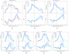 |
Fig. D.2. Same as Fig. D.1 but for anti-aligned angular momenta of clouds’ orbits in the BLR of larger SMBH. (a) 𝒞, i0 = 45° ,Ω1 = 100° ,Ω2 = 300°, ω1 = 250° ,ω2 = 70°, ic1 = rnd(90° ,175° ), ic2 = rnd(−45° ,45° ), Ωc1 = 300°, Ωc2 = 100° ,ωc1 = 170°, ωc2 = 350°, ec = 0.5, (b) 𝒞, i0 = 45°, Ω1 = 100°, Ω2 = 300°, ω1 = 250° ,ω2 = 70°, ek = 1, 2 = (0.5, 0.1),δek = 1, 2 = −0.1, ic1 = rnd(90° ,175° ), ic2 = rnd(−45° ,45° ), Ωc1 = 300°, Ωc2 = 100°, ωc1 = 170° ,ωc2 = 350°, ec = (0.1, 0.5),δec = 0.1, (c) i0 = 45°, i = 10° ,Ω1 = 100°, Ω2 = 300° ,ω1 = 250°, ω2 = 70° ,ek = 1, 2 = 𝒰(0.5, 0.1), δek = 1, 2 = −0.1, ic1 = rnd(90° ,175° ), ic2 = rnd(−45° ,45° ), Ωc1 = 300° ,Ωc2 = 100°, ωc1 = 170°, ωc2 = 350° ,ec = =𝒰(0.1, 0.5), δec = 0.1, (d) i = 10°, Ω1 = 100° ,Ω2 = 300°, ω1 = 250° ,ω2 = 70°, ek = 0.5, k = 1, 2, ic1 = rnd(90° ,175° ), ic2 = rnd(−45° ,45° ), Ωc1 = 300° ,Ωc2 = 100°, ωc1 = 170° ,ωc2 = 350°, ec = 0.5, (e) Ω1 = 100° ,Ω2 = 300° ,ω1 = 250°, ω2 = 70°, ek = 1, 2 = 0.5, ic1 = rnd(90° ,175° ), ic2 = rnd(−45° ,45° ), Ωc1 = 300° ,Ωc2 = 100°, ωc1 = 170° ,ωc2 = 350°, ec = 0.5, (f) Ω1 = 100° ,Ω2 = 300°, ω1 = 250° ,ω2 = 70°, ek = rnd(0.1, 0.5),k = 1, 2, ic1 = rnd(90° ,175° ), ic2 = rnd(−45° ,45° ), Ωc1 = 300°, Ωc2 = 100° ,ωc1 = 170°, ωc2 = 350° ,ec = rnd(0.1, 0.5), (g) Ω1 = 100°, Ω2 = 300°, ω1 = 250° ,ω2 = 70°, ek = rnd(0.1, 0.5),k = 1, 2, ic1 = rnd(90° ,175° ), ic2 = rnd(−45° ,45° ), Ωc1 = 300°, Ωc2 = 100°, ωc1 = 170° ,ωc2 = 350°, ec = ek = 1, 2. |
Effects of the asynchronous orientation of the angular momenta of clouds’ orbit in both BLRs (see Fig. D.3) differs from the previous two cases. The “Eiffel Tower” spectral shapes in Figs. D.3a and D.2g are similar, yet distinct in their left wings. This is reflecting a difference in Ω of clouds and SMBHs orbits. Figure D.5 summarises, in more detail, the simulations for different combinations of ℛ distributions of clouds’ eccentricities and orbital parameters of SMBHs. Also, a notable level of noise is present in the differential phase.
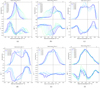 |
Fig. D.3. Same as Fig. D.2 but for anti-aligned angular momenta of clouds in both BLRs. Clouds’ orbital inclinations are randomly distributed within the range (90° ,175°). (a) Ωk = 300° ,ek = rnd(0.1, 0.5),k = 1, 2, ω1 = 250° ω2 = 70° ,Ωc1 = 300° ,Ωc2 = 300°, ωc1 = 170°, ωc2 = 350° , ec = rnd(0.1, 0.5), (b) Ω1 = 300° ,Ω2 = 100°, ek = 0.5, k = 1, 2, ω1 = 250° ω2 = 70°, Ωc1 = 100° ,Ωc2 = 300°, ωc1 = 350° ,ωc2 = 170°, ec = 0.5, (c) i0 = 45°, Ω1 = 100°, Ω2 = 300°, ek = (0.1, 0.5), k = 1, 2, ω1 = 250°, ω2 = 70° ,Ωc1 = 100°, Ωc2 = 300° ,ωc1 = 350°, ωc2 = 170°, (d) i0 = 45° ,Ω1 = 100°, Ω2 = 300° ,ω1 = 250°, ω2 = 70° ,Ωc1 = 100°, Ωc2 = 300°, ωc1 = 350° ,ωc2 = 170°, (e) Ω1 = 350° ,Ω2 = 100°, ω1 = 230° ,ω2 = 50°, ek = 0.5, k = 1, 2, ec = rnd(0.1, 0.5), Ωc = ωc = rnd(10° ,290° ), (f) Ω1 = 350°, Ω2 = 300° ,ω1 = 50°, ω2 = 230° ,ek = 0.5, k = 1, 2, Ωc1 = 100° ,Ωc2 = rnd(10° ,290° ), ωc1 = 100° ,ωc2 = 280°, ec = 0.5. |
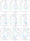 |
Fig. D.4. Simulated interferometric observables for the CB-SMBH system during three orbital phases. From first to third column: Θ(t) = (0, 0.25) with an increment of 0.5. Varying orbital parameters are listed in legends and sub-captions. (a) A0 = 100ld, i0 = i = (10° −40° ,45° ), Ω1 = 200° ,Ω2 = 150°, ek = 0.5, k = 1, 2, ω1 = 70° ,ω2 = 250°, ic1 = ic2 = (10° −40° ,45° ), Ωc1 = Ωc2 = 200°, ωc1 = 100° ,ωc2 = 280° ,ec = 0.5, (b) A0 = 100ld, i0 = i = (10° −40° ,45° ), Ω1 = 200° ,Ω2 = 150°, e1 = (0.1, 0.5),e2 = (0.5, 0.1), ω1 = 70° ,ω2 = 250° ,ic1 = ic2 = (10° −40° ,45° ), Ωc1 = Ωc2 = 200°, ωc1 = 100° ,ωc2 = 280°, ec1 = e2, ec2 = e1, (c) A0 = 100ld, i0 = i = (10° −40° ,45° ), Ω1 = 200° ,Ω2 = 150°, e1 = (0.1, 0.5),e2 = (0.5, 0.1), ω1 = 70° ,ω2 = 250°, ic1 = ic2 = rnd(90° −175° ,45° ), Ωc1 = Ωc2 = 200°, ωc1 = 100° ,ωc2 = 280°, ec1 = e2, ec2 = e1. |
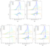 |
Fig. D.5. Evolution of the Paα emission line (upper subplots) and corresponding differential phase (Δϕ, lower subplots) for the CB-SMBH system as a function of the wavelength and radial velocity. The clouds’ orbital eccentricities are drawn from Rayleigh distribution. Varying parameters are listed in sub-captions and legends, and 𝒞 stands for coplanar orbits. (a) 𝒞, Ωk = 100° , ω1 = 110° ,ω2 = 290° ,ic = 𝒰(−5° ,5° ), Ωc1 = 200° , Ωc2 = 10° , ωc1 = 150° ,ωc2 = 330° ,ec1 = ec2 = rndℛ(1), (b) 𝒞, Ωk = 100°, k = 1, 2, ω1 = 110° ,ω2 = 290° ,𝒞, Ωc1 = 200° ,Ωc2 = 10°, ωc1 = 150° ,ωc2 = 330°, ec1 = ec2 = rndℛ(1), (c) 𝒞, Ωk = 100°, k = 1, 2, ω1 = 110°, ω2 = 290° ,ic1 = 𝒞, ic2 = 𝒰(−5° ,5° ), Ωc1 = 200° ,Ωc2 = 10° , ωc1 = 150°, ωc2 = 330° ,ec1 = rndℛ(1), ec2 = 0.5, (d) 𝒞, Ωk = 100°, k = 1, 2, ω1 = 110° ,ω2 = 290°, ic1 = 𝒞, ic2 = 𝒰(−5° ,5° ), Ωc1 = 200° , Ωc2 = 10°, ωc1 = 150° ,ωc2 = 330°, ec1 = ec2 = rndℛ(1), (e) 𝒞, Ωk = 100°, k = 1, 2, ω1 = 110° ,ω2 = 290°, ic1 = ic2 = 𝒰(−5° ,5° ), Ωc1 = 200° ,Ωc2 = 10°, ωc1 = 150° ,ωc2 = 330°, ec1 = 0.5, ec2 = rndℛ(1). |
When motion of clouds in both BLRs are non-coplanar, then the differential phase is slightly deformed in the right-wing (see Fig. D.5b). In addition, if the clouds’ orbital eccentricities in one of the BLRs are high (0.5), then the differential phase shape will be smoother (see Figs. D.5c and D.5e). The same situation is for the coplanar clouds’ motion (see Fig. D.5c). Simulation results for Γs(0.3, 1) distribution of clouds’ eccentricities are given in Fig. D.6. For the coplanar clouds’ motion around a more massive component, the differential phase amplitude decreases (Figs. D.6b–D.6d).
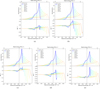 |
Fig. D.6. Same as Fig. D.5 but for clouds’ orbital eccentricities drawn from scaled and shifted Γs(0.3, 1) distribution. (a) 𝒞, Ωk = 100° ,ω1 = 110°, ω2 = 290° ,ic = 𝒰(−5° ,5° ), Ωc1 = 200° ,Ωc2 = 10°, ωc1 = 150° ,ωc2 = 330°, ec1 = ec2 = rndΓs(0.3, 1), (b) 𝒞, Ωk = 100°, k = 1, 2, ω1 = 110° ,ω2 = 290°, ic1 = 𝒰(−5° ,5° ), ic2 = 𝒞, Ωc1 = 200° ,Ωc2 = 10°, ωc1 = 150° ,ωc2 = 330°, ec1 = rndΓs(0.3, 1),ec2 = 0.5, (c) 𝒞, Ωk = 100° , k = 1, 2, ω1 = 110° ,ω2 = 290° ,ic1 = 𝒞, ic2 = 𝒰(−5° ,5° ), Ωc1 = 200° ,Ωc2 = 10°, ωc1 = 150° ,ωc2 = 330°, ec1 = rndΓs(0.3, 1),ec2 = 0.5, (d) 𝒞, Ωk = 100°, k = 1, 2, ω1 = 110° ,ω2 = 290°, ic1 = 𝒰(−5° ,5° ), ic2 = 𝒞, Ωc1 = 200°, Ωc2 = 10° ,ωc1 = 150°, ωc2 = 330° ,ec1 = ec2 = rndΓs(0.3, 1), (e) 𝒞, Ωk = 100° ,k = 1, 2, ω1 = 110°, ω2 = 290° ,ic1 = 𝒰(−5° ,5° ), ic2 = 0, Ωc1 = 200°, Ωc2 = 10°, ωc1 = 150° ,ωc2 = 330°, ec1 = 0.5, ec2 = rndΓs(0.3, 1). |
With the disfigured core of the spectral lines, the net effect is that the differential phase peaks shift away from the line centre because of the smaller contribution of lower velocities of clouds. In such cases, the plateau between differential phase peaks is more prominent. The opposite effect occurs when there are higher contributions of projected lower velocities in spectral lines and, consequently, in the phase profiles.
All Tables
Qualitative summary of simulation parameters effects on the morphology of differential phase (DP) curves for a single SMBH.
Qualitative summary of simulation parameters effects on the morphology of differential phase (DP) curves for CB-SMBH systems.
Parameter sets used in testing the differential phase sensitivity for CB-SMBH based on Eq. (A.4).
All Figures
|
Fig. 1. Realisation of a coplanar elliptical CB-SMBH system with clouds in non-coplanar orbits in both BLRs calculated from the model. M1 and M2 show the locations of the SMBHs in a binary system. Blue ellipses are every 20th of the 100 orbits of clouds in each BLR. The SMBH parameters are M1 = 6 ⋅ 107 M⊙, M2 = 4 ⋅ 107 M⊙, A0 = 100, Ω1 = Ω2 = 3° , ω1 = 1° , ω2 = 181° , e1 = e2 = 0.5. Clouds parameters are Ωc1 = Ωc2 = 180° , ωc1 = 2° , ωc2 = 182° , i = ( − 40° ,40° ), e = 0.5, but their orbital planes have different inclinations. The reference plane (BXY) is the plane of the relative orbit of M2 to M1, and the origin of the coordinate system is the barycentre (B) of the CB-SMBH system. (a) Elevation view of the CB-SMBH system. (b) Side view to the YBZ coordinate plane. |
| In the text | |
|
Fig. 2. Radial velocity maps of simulated images of the BLRs around the primary and secondary components in CB-SMBH. Abscissas (X) and ordinates (Y) are normalised by 𝒜0 = 100ld. The clouds’ orbital angular momenta alignment with CB-SMBH orbital angular momentum is indicated in legends. (a) A0 = 175ld, i0 = 40°, i = 80°, ld, Ω1 = 300°, Ω2 = 50°, ek = 0.5, k = 1, 2, ω1 = 70°, ω2 = 250°, ic1 = ic2 = 40°, Ωc1 = Ωc2 = 300°, ωc1 = 70°, ωc2 = 250°, ec = 0.5, (b) A0 = 175ld, i0 = 40°, i = 80°, Ω1 = 300°, Ω2 = 50°, ek = 0.5, k = 1, 2, ω1 = 70°, ω2 = 250°, ic1 = (90° ,175° ), ic2 = 40°, Ωc1 = Ωc2 = 300°, ωc1 = 70°, ωc2 = 250°, ec = 0.5, (c) A0 = 175, i0 = 40°, i = 80°, ld, Ω1 = 300°, Ω2 = 50°, ek = 0.5, k = 1, 2, ω1 = 70° ω2 = 250°, ic1 = 40°, ic2 = (90° ,175° ), Ωc1 = Ωc2 = 300°, ωc1 = 60°, ωc2 = 240°, ec = 0.5, (d) A0 = 175, i0 = 40°, i = 80°, ld, Ω1 = 300°, Ω2 = 50°, ek = 0.5, k = 1, 2, ω1 = 70° ω2 = 250°, ic1 = ic2 = (90° ,175° ), ωc1 = ωc2 = 300°, ωc1 = 60°, ωc2 = 240°, ec = 0.5. |
| In the text | |
|
Fig. 3. Evolution of the Paα emission line (upper subplots) and corresponding differential phase (Δϕ, lower subplots) as a function of the wavelength for different values of clouds’ orbital parameters in the different models of single SMBH. Common parameters for all models: (a) and (b) clouds’ orbital inclination ic ∈ [ − 5° ,5° ], clouds’ orbital eccentricity ec = 0.5 and i0 = 45°. (c) Clouds’ orbital inclination ic = 𝒰(−7.5° ,7.5° ), and i0 = 𝒰(10° ,45° ). Varying parameters are given in subcaptions. Here, ℑ = 𝒰(l, r) stands for collection of inclination ranges from 𝒰(−l, l) up to 𝒰(−r, r). For reference, interferometric observables marked with blue colour were modelled for values at the lower end of the parameters ranges. (a) Ωc ∈ 𝒰(10° ,180° ), ωc = 110°, (b) Ωc = 100°, ωc = 𝒰(10° ,180° ), (c) ωc = 200°. |
| In the text | |
|
Fig. 4. Same as Fig. 3 but for random samples of clouds’ orbital eccentricities generated from Γs(0.3, 1) and ℛ(1) distributions. Varying parameters are listed in subcaptions and 𝒞 stands for coplanar clouds orbits. (a) i0 = 𝒰(−10° ,45° ), δi0 = 5°, 𝒞, Ωc = 100°, ωc = 270° ,ec ∈ Γs(0.3, 1), (b) i0 = 𝒰(−10° ,45° ), δi0 = 5°, ic = 𝒰(−20° ,20° ), Ωc = 100°, ωc = 270°, ec ∈ ℛ(1). |
| In the text | |
|
Fig. 5. Evolution of the Paα emission line (upper subplots) and the corresponding differential phase (Δϕ, lower subplots) as a function of the wavelength for different values of model parameters for an aligned CB-SMBH system. Orbital elements that are the same for all clouds in both BLR are designated by the subscript, c. Varying parameters are listed in sub-captions; 𝒞 stands for the coplanar CB-SMBH system. (a) i0 = 45° ; ik = 𝒰(90° ,10° ), δik = −10°, Ω1 = 200°, Ω2 = 100°, ωk = 210°, ek = 0.5, k = 1, 2; 𝒥 = 𝒰(5° ,45° ), δ𝒥 = 5°, Ωc = 200°, ωc1 = 150°, ωc2 = 210°, ec = 0.5, (b) i0 = 𝒰(15° ,45° ), δi0 = 5, 𝒞, Ωk = 𝒰(170° ,230° ), δΩk = 20° ωk = 𝒰(270° ,170° ), δωk = −20°, δek = (0.1, 0.5), δek = 0.1, k = 1, 2, ic = 𝒰(−5° ,5° ), Ωc = 𝒰(20° ,160° ), δΩc = 20, ωc = 𝒰(120° ,20° ), δωc = 20°, ec = ek. |
| In the text | |
|
Fig. 6. Same as Fig. 5, but for anti-aligned angular momenta of clouds in the BLR of less massive SMBHs. (a) 𝒞, Ω1 = 100°, Ω2 = 300°, ω1 = 250°, ω2 = 70°, ek = 0.5, k = 1, 2; ic1 = rnd(10° ,45° ), ic2 = rnd(90° ,175° ), Ωc = ωc = rnd(0.1° ,359° ,ec = 0.5, (b) 𝒞, Ω1 = 100°, Ω2 = 300° ,ω1 = 250°, ω2 = 70°, ek = 0.5, k = 1, 2; ic1 = rnd(10° ,45° ), ic2 = rnd(90° ,175° ), Ωc1 = 300°, Ωc2 = 100°, ωc1 = 170°, ωc2 = 350°, ec = 0.5, (c) 𝒞, Ω1 = 100°, Ω2 = 300°, ω1 = 250°, ω2 = 70°; ic1 = rnd(10° ,45° ), ic2 = rnd(90° ,175° ), Ωc1 = 300°, Ωc2 = 100° ,ωc1 = 170°, ωc2 = 350°. |
| In the text | |
|
Fig. 7. Evolution of the Paα emission line (upper subplots) and corresponding differential phase (Δϕ, lower subplots) as a function of the wavelength for aligned CB-SMBH system when the clouds’ orbital eccentricities are drawn from non-uniform distributions; (a) clouds’ orbital eccentricites are drawn from Rayleigh distribution; (b) clouds’ orbital eccentricities are drawn from scaled and shifted Γs(0.3, 1) distributions. (a) 𝒞, Ωk = 100°, k = 1, 2, ω1 = 110°, ω2 = 290°, ic1 = 𝒰(−5° ,5° ), ic2 = 𝒞, Ωc1 = 200°, Ωc2 = 10°, ωc1 = 150°, ωc2 = 330°, ec1 = ec2 = rndℛ(1), (b) 𝒞, Ωk = 100° ,k = 1, 2, ω1 = 110° ,ω2 = 290°, Ωc1 = 200° ,Ωc2 = 10°, ωc1 = 150°, ωc2 = 330°, ic1 = ic2 = 𝒰(−5° ,5° ), ec1 = 0.5, ec2 = rndΓs(0.3, 1). |
| In the text | |
|
Fig. A.1. Interactive effects of clouds’ orbital elements on the values of the first parameter in Eq. (A.2) present as the surface mesh. (a) X axis shows the clouds’ ascending node Ω, the y axis shows the true anomaly (f), z axis shows values of the calculated parameter for fixed elements ω = π/3, i = π/3, e = 0.5, a = 15 ld. (b) X axis shows the clouds’ orbital inclination and fixed elements are ω = 4.66 rad, f = 3.38 rad, e = 0.19. (c) X axis shows the eccentricity and fixed elements are ω = 11π/18, Ω = 10π/18, f = 0 rad. |
| In the text | |
|
Fig. A.2. Surface mesh of the values of the first parameter in Eq. (13) over a grid of orbital elements of larger SMBH. The ascending node Ω1 and true anomaly f1 are given in the XY coordinate plane, and values of the calculated parameter are given on the Z-axis. Upper left plot: Case I – parameters are listed in Table A.1a. Upper right plot: Case II – parameters are listed in Table A.1b. Bottom left: Case III – parameters are listed in Table A.1c. Bottom right: Case IV – parameters are listed in Table A.1d. |
| In the text | |
|
Fig. B.1. Evolution of the Paα emission line (upper subplots) and corresponding differential phase (Δϕ, lower subplots) as a function of the wavelength and radial velocity for different values of the clouds’ orbital parameters in the model of single SMBH. Model parameters are given in the sub-captions. (a) Ωc ∈ 𝒰(10° ,90° ), ωc = 110°, ic ∈ 𝒰(−5° ,5° ), ec = 0.5, i0 = 45°, (b) ic = 𝒰(−5° ,5° ), Ωc = 100°, ωc = 10°, i0 = 45°, ec = 𝒰(0.1, 0.5), (c) ic = 𝒰(−5° ,5° ), Ωc = 100°, ωc = 110°, i0 = 45°, ec = 𝒰(0.1, 0.5), (d) ic = 𝒰(−5° ,5° ), Ωc = 100°, ec = 0.5, ωc = 270°, i0 = 𝒰(10° ,45° ). |
| In the text | |
|
Fig. B.2. Same as Fig. B.1 but for fixed values of clouds’ orbital eccentricities, ec = 0.5, and angular position of observer, i0 = 45°. (a), (b) Ωc = 100°. The range of the clouds’ orbital inclinations for each model is from 𝒰(−5°, 5°) to 𝒰(−20°, 20°). (a) ωc = 10, (b) ωc = 110°, (c) Ω = 210°, ωc = 10°, ec = 0.5, ic = 𝒰(−7.5° ,7.5° ), i0 = 𝒰(10° ,45° ). |
| In the text | |
|
Fig. B.3. Same as Fig. B.1 but for the range of clouds’ orbital inclinations from 𝒰(−5°, 5°) to 𝒰(−20°, 20°), with fixed values of the clouds’ orbital eccentricities, ec = 0.5, and i0 = 15°. The rest of the parameters are given in the sub-captions of the plots. (a) ωc = 10°, (b) ωc = 110°, (c) ic = 𝒰(−40° ,40° ), i0 = 45°, ωc = (10° ,180° ). |
| In the text | |
|
Fig. B.4. Same as Fig. B.1 but for random samples of clouds’ orbital eccentricities generated from Γs(0.3, 1) and ℛ(1) distributions. Varying parameters are listed in sub-captions. 𝒞 stands for coplanar clouds orbits. (a) i0 = 𝒰(−10° ,45° ), δi0 = 5°, ic = 𝒰(−20° ,20° ), Ωc = 100°, Ωc = 270°, ec ∈ Γs(0.3, 1), (b) i0 = 𝒰(−10° ,45° ), δi0 = 5°, 𝒞, Ωc = 100°, ωc = 270°, ec ∈ ℛ(1), (c) i0 = 𝒰(−10° ,45° ), δi0 = 5°, ic = 𝒰(−10° ,10° ), Ωc = 100°, ωc = 10°, ec ∈ ℛ(1), (d) i0 = 𝒰(−10° ,45° ), δi0 = 5°, 𝒞, Ωc = 100°, ωc = 10°, ec ∈ Γs(0.3, 1), (e) i0 = 𝒰(−10° ,45° ), δi0 = 5° ,ic = ( − 7.5° ,7.5° ), Ωc = 100°, ωc = 10°, ec ∈ Γs(0.3, 1), (f) i0 = 𝒰(−10° ,45° ), δi0 = 5°, 𝒞, Ωc = 100° ,ωc = 10°, ec ∈ ℛ(1). |
| In the text | |
|
Fig. C.1. Evolution of the Paα emission line (upper subplots) and corresponding differential phase (Δϕ, lower subplots) as a function of the wavelength radial velocity for different models of aligned CB-SMBH system. Common clouds’ orbital elements are designed by subscript c. 𝒞 stands for the coplanar CB-SMBH system. ℑ = 𝒰(l, r) stands for inclination ranges from 𝒰(−l, l) up to 𝒰(−r, r). (a) i0 = 45° ;𝒞, Ωk = 100°, ωk = 110°, ek = 𝒰(0.05, 0.1 − 0.4, 0.45), k = 1, 2, δek = 0.1; ic = 𝒰(−5° ,5° ), Ωc = 10°, ωc = 180°, |
| In the text | |
|
Fig. C.2. Same as Fig. C.1 but for different SMBHs and clouds’ orbital parameters. Plot (c): rnd stands for randomly chosen samples of orbital elements. ℑ = 𝒰(l, r) stands for inclination ranges from 𝒰(−l, l) up to 𝒰(−r, r). (a) i0 = 45° ;ik = 𝒰(10° ,90° ), δik = 10°, Ωk = 200°, ωk = 210°, ek = 0.5, k = 1, 2; 𝒥 = 𝒰(5° ,45° ), δ𝒥 = 5°, Ωc = 200°, ωc1 = 290° ,ωc2 = 210°, ec = 0.5, (b) i0 = 45° ;ik = 𝒰(90° ,10° ), δik = −10°, Ωk = 200°, ωk = 210°, ek = 0.5, k = 1, 2; 𝒥 = 𝒰(5° ,45° ), δ𝒥 = 5°, Ωc = 200°, ωc1 = 290°, ωc2 = 210° ,ec = 0 : 5, (c) i0 = 45° ;ik = 𝒰(10° ,90° ), δik = −10°, Ω1 = 200°, Ω2 = 100°, ωk = 210°, ek = 0.5, k = 1, 2; Ωc = 200° ,ωc1 = 150°, ωc2 = 210° ,ic1 = rnd(5° ,45° ), ic1 = (5° ,45° ), ec = 0.5, (d) i0 = 45° ;ik = 𝒰(90° ,10° ), δik = −10° ,Ωk = 5°, ω1 = 5°, ω2 = 180°, ek = 0.5, k = 1, 2; 𝒥 = 𝒰(5° ,45° ), δ𝒥 = 5°, ec = 0.5, Ωc = 100°, ωc1 = 5°, ωc2 = 180°, (e) i0 = 45° ;ik = 𝒰(5° ,45° ), δik = 10°, Ωk = 5°, ω1 = 5°, ω2 = 180° ,ek = 0.5, k = 1, 2; 𝒥 = 𝒰(5° ,45° ), δ𝒥 = 5°, Ωc = 100°, ωc1 = 5°, ωc2 = 180°, ec = 0.5. |
| In the text | |
|
Fig. C.3. Same as Fig. C.1 but for different SMBHs and clouds’ orbital parameters. (a) i0 = 𝒰(10° ,45° ), δi0 = 5° ;ik = (10° ,90° ), δik = −10°, Ωk = 5°, ω1 = 5°, ω2 = 180°, ek = 0.5, k = 1, 2; 𝒥 = 𝒰(10° ,45° ), δ𝒥 = 5°, Ωc = 100° ,ωc1 = 5°, ωc2 = 180° ,ec = 0.5, (b) i0 = 𝒰(15° ,45° ), δi0 = 5° ;ik = 𝒰(80° ,20° ), δik = −10° ,Ωk = 𝒰(230° ,330° ), δΩk = 20°, ωk = 𝒰(270° ,170° ), δωk = 20° ,ek = 0.5, k = 1, 2; 𝒥 = 𝒰(5° ,45° ), δ𝒥 = 5°, Ωc = 𝒰(80° ,180° ), δΩc = 20, ωc = 𝒰(120° ,20° ), δωc = 20° ,ec = 0.5, (c) i0 = 45° ;ik = 𝒰(10° ,90° ), δik = 10° ,Ωk = 5°, ω1 = 5° , ω2 = 180°, ek = 0.2, k = 1, 2;𝒥 = 𝒰(5° ,45° ), δ𝒥 = 5°, Ωc = 200° ,ωc1 = 290°, ωc2 = 210° ,ec = 0.2, (d) i0 = 45° ;ik = 5°, Ωk = 𝒰(20° ,180° ), δΩk = 20°, ωk = 𝒰(180° ,20° ), δωk = −20°, ek = 0.5, k = 1, 2; ic = 5° ,Ωc = Ωk, ωc1 = ωk, ec = 0.5, (e) i0 = 𝒰(20° ,45° ), δi0 = 5° ;ik = 10°, Ωk = 𝒰(230° ,330° ), δΩk = 20°, ωk = 𝒰(270° ,190° ), δωk = −20°, ek = 0.5, k = 1, 2; ic = 5°, Ωc = 𝒰(80° ,180° ), δΩk = 20° ,ωc1 = 𝒰(120° ,20° ), δωk = −20° ,ec = 0.5. |
| In the text | |
|
Fig. D.1. Same as Fig. C.1 but for anti-aligned angular momenta of clouds in the BLR of less massive SMBH. (a) 𝒞.Ωk = 100° ,ω1 = 250°, ω2 = 70° ,ek = 0.5, k = 1, 2; ic1 = 𝒰(−5° ,5° ), ic2 = 𝒰(90° ,175° ), Ωc = rnd(0.1° ,359° ), ωc1 = 120° ,ωc2 = 300° ,ec = 0.5, (b) 𝒞, Ωk = 100°, ω1 = 250°, ω2 = 70°, ek = 0.5, k = 1, 2; 𝒥 = 𝒰(10° ,45° ), δ𝒥 = 5° ,ic2 = 𝒰(90° −175° ), Ωc = ωc = rnd(0.1° ,359° ), ec = 0.5, (c) 𝒞, Ω1 = 100°, Ω2 = 300° ,ω1 = 100°, ω2 = 180°, ek = 0.5, k = 1, 2; 𝒥 = (10° ,45° ), δ𝒥 = 5°, ic2 = 𝒰(90° 175° ), Ωc = rnd(0.1° ,359°, ωc1 = 220° ,ωc2 = 40°, ec = rnd(0.1, 0.5). |
| In the text | |
|
Fig. D.2. Same as Fig. D.1 but for anti-aligned angular momenta of clouds’ orbits in the BLR of larger SMBH. (a) 𝒞, i0 = 45° ,Ω1 = 100° ,Ω2 = 300°, ω1 = 250° ,ω2 = 70°, ic1 = rnd(90° ,175° ), ic2 = rnd(−45° ,45° ), Ωc1 = 300°, Ωc2 = 100° ,ωc1 = 170°, ωc2 = 350°, ec = 0.5, (b) 𝒞, i0 = 45°, Ω1 = 100°, Ω2 = 300°, ω1 = 250° ,ω2 = 70°, ek = 1, 2 = (0.5, 0.1),δek = 1, 2 = −0.1, ic1 = rnd(90° ,175° ), ic2 = rnd(−45° ,45° ), Ωc1 = 300°, Ωc2 = 100°, ωc1 = 170° ,ωc2 = 350°, ec = (0.1, 0.5),δec = 0.1, (c) i0 = 45°, i = 10° ,Ω1 = 100°, Ω2 = 300° ,ω1 = 250°, ω2 = 70° ,ek = 1, 2 = 𝒰(0.5, 0.1), δek = 1, 2 = −0.1, ic1 = rnd(90° ,175° ), ic2 = rnd(−45° ,45° ), Ωc1 = 300° ,Ωc2 = 100°, ωc1 = 170°, ωc2 = 350° ,ec = =𝒰(0.1, 0.5), δec = 0.1, (d) i = 10°, Ω1 = 100° ,Ω2 = 300°, ω1 = 250° ,ω2 = 70°, ek = 0.5, k = 1, 2, ic1 = rnd(90° ,175° ), ic2 = rnd(−45° ,45° ), Ωc1 = 300° ,Ωc2 = 100°, ωc1 = 170° ,ωc2 = 350°, ec = 0.5, (e) Ω1 = 100° ,Ω2 = 300° ,ω1 = 250°, ω2 = 70°, ek = 1, 2 = 0.5, ic1 = rnd(90° ,175° ), ic2 = rnd(−45° ,45° ), Ωc1 = 300° ,Ωc2 = 100°, ωc1 = 170° ,ωc2 = 350°, ec = 0.5, (f) Ω1 = 100° ,Ω2 = 300°, ω1 = 250° ,ω2 = 70°, ek = rnd(0.1, 0.5),k = 1, 2, ic1 = rnd(90° ,175° ), ic2 = rnd(−45° ,45° ), Ωc1 = 300°, Ωc2 = 100° ,ωc1 = 170°, ωc2 = 350° ,ec = rnd(0.1, 0.5), (g) Ω1 = 100°, Ω2 = 300°, ω1 = 250° ,ω2 = 70°, ek = rnd(0.1, 0.5),k = 1, 2, ic1 = rnd(90° ,175° ), ic2 = rnd(−45° ,45° ), Ωc1 = 300°, Ωc2 = 100°, ωc1 = 170° ,ωc2 = 350°, ec = ek = 1, 2. |
| In the text | |
|
Fig. D.3. Same as Fig. D.2 but for anti-aligned angular momenta of clouds in both BLRs. Clouds’ orbital inclinations are randomly distributed within the range (90° ,175°). (a) Ωk = 300° ,ek = rnd(0.1, 0.5),k = 1, 2, ω1 = 250° ω2 = 70° ,Ωc1 = 300° ,Ωc2 = 300°, ωc1 = 170°, ωc2 = 350° , ec = rnd(0.1, 0.5), (b) Ω1 = 300° ,Ω2 = 100°, ek = 0.5, k = 1, 2, ω1 = 250° ω2 = 70°, Ωc1 = 100° ,Ωc2 = 300°, ωc1 = 350° ,ωc2 = 170°, ec = 0.5, (c) i0 = 45°, Ω1 = 100°, Ω2 = 300°, ek = (0.1, 0.5), k = 1, 2, ω1 = 250°, ω2 = 70° ,Ωc1 = 100°, Ωc2 = 300° ,ωc1 = 350°, ωc2 = 170°, (d) i0 = 45° ,Ω1 = 100°, Ω2 = 300° ,ω1 = 250°, ω2 = 70° ,Ωc1 = 100°, Ωc2 = 300°, ωc1 = 350° ,ωc2 = 170°, (e) Ω1 = 350° ,Ω2 = 100°, ω1 = 230° ,ω2 = 50°, ek = 0.5, k = 1, 2, ec = rnd(0.1, 0.5), Ωc = ωc = rnd(10° ,290° ), (f) Ω1 = 350°, Ω2 = 300° ,ω1 = 50°, ω2 = 230° ,ek = 0.5, k = 1, 2, Ωc1 = 100° ,Ωc2 = rnd(10° ,290° ), ωc1 = 100° ,ωc2 = 280°, ec = 0.5. |
| In the text | |
|
Fig. D.4. Simulated interferometric observables for the CB-SMBH system during three orbital phases. From first to third column: Θ(t) = (0, 0.25) with an increment of 0.5. Varying orbital parameters are listed in legends and sub-captions. (a) A0 = 100ld, i0 = i = (10° −40° ,45° ), Ω1 = 200° ,Ω2 = 150°, ek = 0.5, k = 1, 2, ω1 = 70° ,ω2 = 250°, ic1 = ic2 = (10° −40° ,45° ), Ωc1 = Ωc2 = 200°, ωc1 = 100° ,ωc2 = 280° ,ec = 0.5, (b) A0 = 100ld, i0 = i = (10° −40° ,45° ), Ω1 = 200° ,Ω2 = 150°, e1 = (0.1, 0.5),e2 = (0.5, 0.1), ω1 = 70° ,ω2 = 250° ,ic1 = ic2 = (10° −40° ,45° ), Ωc1 = Ωc2 = 200°, ωc1 = 100° ,ωc2 = 280°, ec1 = e2, ec2 = e1, (c) A0 = 100ld, i0 = i = (10° −40° ,45° ), Ω1 = 200° ,Ω2 = 150°, e1 = (0.1, 0.5),e2 = (0.5, 0.1), ω1 = 70° ,ω2 = 250°, ic1 = ic2 = rnd(90° −175° ,45° ), Ωc1 = Ωc2 = 200°, ωc1 = 100° ,ωc2 = 280°, ec1 = e2, ec2 = e1. |
| In the text | |
|
Fig. D.5. Evolution of the Paα emission line (upper subplots) and corresponding differential phase (Δϕ, lower subplots) for the CB-SMBH system as a function of the wavelength and radial velocity. The clouds’ orbital eccentricities are drawn from Rayleigh distribution. Varying parameters are listed in sub-captions and legends, and 𝒞 stands for coplanar orbits. (a) 𝒞, Ωk = 100° , ω1 = 110° ,ω2 = 290° ,ic = 𝒰(−5° ,5° ), Ωc1 = 200° , Ωc2 = 10° , ωc1 = 150° ,ωc2 = 330° ,ec1 = ec2 = rndℛ(1), (b) 𝒞, Ωk = 100°, k = 1, 2, ω1 = 110° ,ω2 = 290° ,𝒞, Ωc1 = 200° ,Ωc2 = 10°, ωc1 = 150° ,ωc2 = 330°, ec1 = ec2 = rndℛ(1), (c) 𝒞, Ωk = 100°, k = 1, 2, ω1 = 110°, ω2 = 290° ,ic1 = 𝒞, ic2 = 𝒰(−5° ,5° ), Ωc1 = 200° ,Ωc2 = 10° , ωc1 = 150°, ωc2 = 330° ,ec1 = rndℛ(1), ec2 = 0.5, (d) 𝒞, Ωk = 100°, k = 1, 2, ω1 = 110° ,ω2 = 290°, ic1 = 𝒞, ic2 = 𝒰(−5° ,5° ), Ωc1 = 200° , Ωc2 = 10°, ωc1 = 150° ,ωc2 = 330°, ec1 = ec2 = rndℛ(1), (e) 𝒞, Ωk = 100°, k = 1, 2, ω1 = 110° ,ω2 = 290°, ic1 = ic2 = 𝒰(−5° ,5° ), Ωc1 = 200° ,Ωc2 = 10°, ωc1 = 150° ,ωc2 = 330°, ec1 = 0.5, ec2 = rndℛ(1). |
| In the text | |
|
Fig. D.6. Same as Fig. D.5 but for clouds’ orbital eccentricities drawn from scaled and shifted Γs(0.3, 1) distribution. (a) 𝒞, Ωk = 100° ,ω1 = 110°, ω2 = 290° ,ic = 𝒰(−5° ,5° ), Ωc1 = 200° ,Ωc2 = 10°, ωc1 = 150° ,ωc2 = 330°, ec1 = ec2 = rndΓs(0.3, 1), (b) 𝒞, Ωk = 100°, k = 1, 2, ω1 = 110° ,ω2 = 290°, ic1 = 𝒰(−5° ,5° ), ic2 = 𝒞, Ωc1 = 200° ,Ωc2 = 10°, ωc1 = 150° ,ωc2 = 330°, ec1 = rndΓs(0.3, 1),ec2 = 0.5, (c) 𝒞, Ωk = 100° , k = 1, 2, ω1 = 110° ,ω2 = 290° ,ic1 = 𝒞, ic2 = 𝒰(−5° ,5° ), Ωc1 = 200° ,Ωc2 = 10°, ωc1 = 150° ,ωc2 = 330°, ec1 = rndΓs(0.3, 1),ec2 = 0.5, (d) 𝒞, Ωk = 100°, k = 1, 2, ω1 = 110° ,ω2 = 290°, ic1 = 𝒰(−5° ,5° ), ic2 = 𝒞, Ωc1 = 200°, Ωc2 = 10° ,ωc1 = 150°, ωc2 = 330° ,ec1 = ec2 = rndΓs(0.3, 1), (e) 𝒞, Ωk = 100° ,k = 1, 2, ω1 = 110°, ω2 = 290° ,ic1 = 𝒰(−5° ,5° ), ic2 = 0, Ωc1 = 200°, Ωc2 = 10°, ωc1 = 150° ,ωc2 = 330°, ec1 = 0.5, ec2 = rndΓs(0.3, 1). |
| In the text | |
Current usage metrics show cumulative count of Article Views (full-text article views including HTML views, PDF and ePub downloads, according to the available data) and Abstracts Views on Vision4Press platform.
Data correspond to usage on the plateform after 2015. The current usage metrics is available 48-96 hours after online publication and is updated daily on week days.
Initial download of the metrics may take a while.