| Issue |
A&A
Volume 644, December 2020
|
|
|---|---|---|
| Article Number | A46 | |
| Number of page(s) | 10 | |
| Section | Interstellar and circumstellar matter | |
| DOI | https://doi.org/10.1051/0004-6361/202038632 | |
| Published online | 01 December 2020 | |
Studies of the distinct regions due to CO selective dissociation in the Aquila molecular cloud
1
Xinjiang Astronomical Observatory, Chinese Academy of Sciences,
Urumqi
830011,
PR China
e-mail: This email address is being protected from spambots. You need JavaScript enabled to view it.
; This email address is being protected from spambots. You need JavaScript enabled to view it.
2
University of the Chinese Academy of Sciences,
Beijing
100080,
PR China
3
Department of Solid State Physics and Nonlinear Physics, Faculty of Physics and Technology, Al-Farabi Kazakh National University,
Almaty
050040, Kazakhstan
4
Netherlands Institute for Radio Astronomy,
ASTRON,
7991 PD
Dwingeloo, The Netherlands
e-mail: This email address is being protected from spambots. You need JavaScript enabled to view it.
5
Key Laboratory of Radio Astronomy, Chinese Academy of Sciences,
Urumqi
830011,
PR China
6
The Department of Physics, Faculty of Science, University of Malaya,
50603
Kuala Lumpur, Malaysia
Received:
10
June
2020
Accepted:
26
October
2020
Abstract
Aims. We investigate the role of selective dissociation in the process of star formation by comparing the physical parameters of protostellar-prestellar cores and the selected regions with the CO isotope distributions in photo-dissociation regions. We seek to understand whether there is a better connection between the evolutionary age of star forming regions and the effect of selective dissociation
Methods. We used wide-field observations of the 12CO, 13CO, and C18O (J = 1–0) emission lines to study the ongoing star formation activity in the Aquila molecular region, and we used the 70 and 250 μm data to describe the heating of the surrounding material and as an indicator of the evolutionary age of the core.
Results. The protostellar-prestellar cores are found at locations with the highest C18O column densities and their increasing evolutionary age coincides with an increasing 70μm/250μm emission ratio at their location. The evolutionary age of the cores may also follow from the 13CO versus C18O abundance ratio, which decreases with increasing C18O column densities. The original mass has been estimated for nine representative star formation regions and the original mass of the region correlates well with the integrated 70 μm flux density. Similarly, the X13CO/XC18O ratio, which provides the dissociation rate for these regions correlates with the 70 μm/250 μm flux density ratio and reflects the evolutionary age of the star formation activity.
Key words: ISM: clouds / evolution / ISM: abundances / ISM: molecules / photon-dominated region / stars: formation
© ESO 2020
1 Introduction
The Aquila rift is part of a dark lane of cosmic dust flowing prominently through the central region of the galactic plane of the Milky Way, forming the Great Rift. The two known sites of star formation in the Aquila Rift cloud complex, namely the Serpens South (Bontemps et al. 2010) and the W 40 H II region (Smith et al. 1985), have become a hot spot for the study of star formation. Spitzer observations show that W 40 and the embedded cluster Serpens South are near to one another on the sky, such that the Serpens South is seemingly part of the more evolved W 40 region (Gutermuth et al. 2008). The distance to Serpens Main and W 40 was recently measured to be 436 pc, and the distance to Serpens South should be similar because the two sources are kinematically connected (Ortiz-León et al. 2017). Su et al. (2020) estimated a mass of ∽1.4 × 10⁵ M⊙ for the W 40 giant molecular cloud, and determined a distance of ∽474 pc.
Recently, Könyves et al. (2015) presented the results of the Herschel Gould Belt survey (HGBS) observations in the Aquila molecular cloud AMC complex imaged with the SPIRE and PACS photometric cameras from 70 to 500 μm. These latter authors identified a complete sample of starless dense cores and embedded (Class 0–I) protostars in the AMC complex using the multi-scale, multi-wavelength source-extraction algorithm. In this study, we use the 70 and 250 μm data to describe the heating of the surrounding material and as an indicator of the evolutionary age of the core.
In this work, we encounter regions that are called photo-dissociation regions (PDRs) and regions where we suspect that selective dissociation also plays a role. We investigate the role of selective dissociation in the process of star formation by comparing the physical parameters of protostellar-prestellar cores and the distinct regions with the CO isotope distributions in PDRs. We seek to understand whether or not there is a close relationship between the evolutionary age of star formingregions and the effect of selective dissociation. A detailed description of how selective dissociation works is provided in Sect. 3.6. Breifly, as the star formation process progresses, far-ultraviolet photons start to regulate both the heating and the chemistry of the resulting PDR (Tielens & Hollenbach 1985). Selective dissociation of CO is an expected phenomenon in PDRs resulting from the UV radiation field (Glassgold et al. 1985; Yurimoto & Kuramoto 2004). In this process, UV radiation selectively dissociates less-abundant CO isotopologues more effectively than more-abundant ones owing to different levels of self-shielding (van Dishoeck & Black 1988; Liszt 2007; Shimajiri et al. 2014). As several regions have been identified as distinct star formation regions in the H2 CO absorption map of the AMC (Komesh et al. 2019), here we compare the C18O distribution and the H2CO absorption.
In the present paper, we show the results of the 12CO, 13CO, and C18O observations toward the W 40 and Serpens South regions of the Aquila Rift. In Sect. 2, we present the details of the observations. The results and discussions are described in Sect. 3. Finally, we present our conclusions in Sect. 4.
2 Archival data
The 12CO(1−0), 13CO (1−0), and C18O (1−0) data, simultaneously observed using the 13.7 m millimeter wave telescope of the Purple Mountain Observatory in Delingha, were taken from the Millimeter Wave Radio Astronomy Database1. The central position of the on-the-fly (OTF) observing pattern is 18h30m03s –2°02′40′′ (J2000). The half-power beam width (HPBW) of the observing system is ∽ 50′′, the velocity resolution is 0.17 km s−1, and the system temperature ranged from 180 to 320 K. The 12CO(1−0), 13CO (1−0), and C 18O (1−0) data were smoothed to the same spatial resolution of 60′′ and the cell size is 30′′. The one-sigma noise levels of the 12CO, 13CO, and C18O data are 0.5, 0.35, and 0.35 K, respectively. Assuming a distance of 436 pc for the Aquila complex, the spatial scale of the maps is 0.124 pc arcmin−1.
Infrared 70 and 250 μm images (André et al. 2010) were obtained from The Herschel Gould Belt Survey Archive2.
3 Results and discussion
3.1 12CO(1–0) emission line
The integrated intensity map of 12CO(1–0) over a velocity range 2 < VLSR < 12 km s−1 with signal-to-noise ratio (S/N) greater than three is presented in Fig. 1a. Enhanced core emission is present around W 40 on the north and west sides, which could result from heating by the H II region. There is weak emissions around Serpens South. The brightest position is at (RA,Dec) = (18h31m15s, −2°08′ 13′′).
3.2 13CO(1–0) emission line
The integrated intensity map of 13CO(1−0) over a velocity range 2 < VLSR < 12 km s−1 and a S/N greater than three is presented in Fig. 1b. Here, enhanced emission is also seen to the north and west of W 40. There are several elongated structures at Serpens South.
3.3 C18O(1–0) emission line
The integrated intensity map of C18O(1−0) over a velocity range 2 < VLSR < 12 km s−1 is presented in Fig. 1c with its S/N greater than three. Several integrated intensity concentrations are present in this map including both the W 40 H II region and Serpens South. The distribution of the C 18O (1−0) emission shows some similarity to the Herschel 250 μm large-scale (∽0.124 pc) image presented in Fig. 1d. Both the C18O and the Herschel data trace the same regions, which suggests that the C18O and the Herschel 250 μm emission arise from similar regions.
3.4 Column densities and abundance ratios
The excitation temperature, Tex, was estimated from the peak brightness temperature of 12CO(1−0), by the following equation with the assumption that the 12CO(1−0) line is optically thick and taking into account a beam-filling factor of one (e.g. Pineda et al. 2010; Kong et al. 2015; Lin et al. 2016):
![Mathematical equation: \begin{equation*} \begin{split} T_{\textrm{ex}}&\,{=}\,\frac{hv_{^{12}\textrm{CO}}}{k}\left[\ln\left(1+\frac{hv_{^{12}\textrm{CO}}/k}{T_{\textrm{mb},^{12}\textrm{CO}}+J_v(T_{\textrm{bg}})} \right)\right]^{-1} \textrm{K} \\ &\,{=}\,5.53\left[\ln\left(1+\frac{5.53}{T_{\textrm{mb},^{12}\textrm{CO}}+0.818} \right)\right]^{-1} \textrm{K}, \end{split} \end{equation*}](/articles/aa/full_html/2020/12/aa38632-20/aa38632-20-eq3.png) (1)
(1)
where  is the peak intensity of 12CO(1−0) in units of K,
  is the effective radiation temperature (Ulich & Haas 1976), and Tbg = 2.7 K is the temperature of cosmic microwave background radiation. The estimated excitation temperatures in the whole observed region range from 3.6 to 23.6 K, but these values are underestimates in locations where the 12CO emission is affected by self-absorption. We assume that the excitation temperatures (Tex) of 13CO and C18O lines have the same value as that of the optically thick 12CO line. The optical depth and the column densities of 13CO(1−0) and C18O(1−0) were estimated using the following equations on the assumption that the cloud is in local thermodynamic equilibrium (LTE; e.g. Lada et al. 1994; Kawamura et al. 1998; Lin et al. 2016):
![Mathematical equation: \begin{equation*} \tau (\textrm{C^{18}O})\,{=}\,{-}\ln\left[1-\frac{T_{\textrm{mb,C}^{18}\textrm{O}}}{5.27[J_1(T_{\textrm{ex}})-0.166]}\right], \end{equation*}](/articles/aa/full_html/2020/12/aa38632-20/aa38632-20-eq6.png) (2)
(2)
![Mathematical equation: \begin{equation*} \tau (\textrm{^{13}CO})\,{=}\,{-}\ln\left[1-\frac{T_{\textrm{mb},^{13}\textrm{CO}}}{ 5.29[J_2(T_{\textrm{ex}})-0.164]}\right] ,\end{equation*}](/articles/aa/full_html/2020/12/aa38632-20/aa38632-20-eq7.png) (3)
(3)
and
 (4)
(4)
 (5)
(5)
where J1(Tex) = 1∕[exp(5.27∕Tex) − 1], J2 (Tex) = 1∕ [exp (5.29∕Tex) − 1], and ΔV is the FWHM in km s−1. The abundance ratio,  , is equivalent to the
  column density ratio.
In the regions where the 12CO emission is affected by self-absorption, the column densities of 13CO and C18O are effected by underestimates of Tex from the 12CO data. This leads to underestimation of the column densities of 13CO and C18O in those areas. The resulting ranges of  and N(C18O) are 3.8 × 10¹⁴–5.5 × 1016 cm−2 and 2 × 10¹⁴–3.4 × 10¹⁵, respectively, and the resulting range of the abundance ratio of R13∕18 is 1.02–41.9. A map of the column density of C18O(1−0) is represented in Fig. 2.
The column density of C18O(1−0) versus the number of pixels with C18O(1−0) is displayed in the diagrams of Fig. 3 together with the observed column densities at the location of the prestellar and protostellar cores. The cores sample locations with increasing C18O column density confirming that star formation first happens in regions with the highest column densities. Most of the C 18O(1−0) detection points correspond to the column densities in the range 0.5 × 10¹⁵–1.6 × 1015 cm−2 (see panel a). The prestellar and protostellar cores correlate well with the C18O column density. The majority of the prestellar cores column densities in the range of 0.5 × 10¹⁵–2 × 1015 cm−2 while the locations of the protostellar cores coincide with the column densities in the range of 0.5 × 10¹⁵–2.8 × 1015 cm−2.
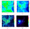 |
Fig. 1 Aquila maps of the intensities of (a) 12CO (1−0), (b) 13CO (1−0), and (c) C 18O (1−0) integrated from 2 to 12 km s−1. White filled circles in the bottom-right corner of each panel illustrate the beam size of 60′′. (d) The Herschel 250 μm image (the beam size is 18.2′′) taken from André et al. (2010). The circle and star mark the locations of the W 40 H II region (radius ∽ 3′) and the Serpens South, respectively. |
3.5 Far-infrared distribution
The peak flux density at the prestellar and protostellar cores at 70 and 250 μm is presented versus the column density of C18O(1−0) diagrams in Fig. 4. The 70 μm diagram (panel a) shows a clear separation indicated with a dotted line between the prestellar and protostellar core distributions; most of prestellar cores have a lower flux density while most of the protostellar cores have a higher flux that may increase slightly at higher column densities. However, excluding the uncertainty on the N(C18O) emission, the 250 μm distribution in panel b shows an increasing trend with column density suggesting that star formation is more advanced athigher column densities and that an increasing volume is affected by the ongoing star formation. Star formation processes are slower in regions of lower column density and more time is required to heat the surrounding environment. In addition, the number of protostellar (or prestellar) cores may be larger because of fragmentation which will accelerate the heating process. The number of cores with very high column density is much smaller than for low-column-density cores, which agrees with the histogram of the stellar core number versus the C18O column density in Fig. 3.
3.6 Selective photodissociation
A map of the abundance ratio  /
/ is presentedin Fig. 5. The contours show the value of
  /
/ = 4. We selected nine unique regions (A–I) in the map where the abundance ratio has a lower value (A, B, C, E, F, and G), one region with a much higher value (region D), and two regions on the outskirts with medium values (H and I). The abundance ratio located in region D next to the W 40 H II region is as high as 42, which is significantly higher than the value of 5.5 seen in the Solar System (Anders & Grevesse 1989). Region D is located next to the W 40 (northwest side), region B is Serpens South, and region G was identified as a distinct star formation region by Komesh et al. (2019). The far-ultraviolet (FUV) emission with sufficient energy to photo-dissociate 12CO promptly becomes optically thick as it penetrates molecular clouds. On the contrary, C18O self-shielding is relatively less significant because of its low abundance and the shift of its absorption lines. Hence, this infers that the FUV emission with higher energy than the C18O dissociation level will penetrate deeper into a molecular cloud and will also increase the abundance ratio of 13CO and C18O,
  /
/ , at the instance when C18O self-shielding is not yet dominant. When both self-shielding effects of 13CO and C18O become significant, the abundance ratio will decrease towards its intrinsic value, which is derived from 12C,13C, 16O, and 18C abundances (van Dishoeck & Black 1988; Liszt 2007; Shimajiri et al. 2014). We can therefore confirm that selective FUV photodissociation of C 18 O indeed occurs.
Figure 6 presents the averaged spectra of 12CO(1−0), 13CO(1−0), and C 18O(1−0) emission in the nine selected regions. The central component of the broader 12CO can clearly be seen to be depleted by self-absorption. However, the spectrum shapes of 13CO and C18O appear different from that of 12CO.
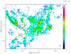 |
Fig. 2 Map of the column density of C18O(1− 0). The black stars and triangles present the locations of protostellar and prestellar cores, respectively. The coordinates of the protostellar and prestellar cores were taken from Könyves et al. (2015). The black circle marks the location of the W 40 H II region (radius ∽ 3′) and the black filled circle in the bottom-right corner illustrates the beam size of 60′′. The clippinglevel for the 13CO and C18O data corresponds to a signal-to-noise ratio greater than five. Gaussian fitting to each pixel was done. |
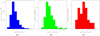 |
Fig. 3 Histograms of the distributions of (a) the number of pixels with certain column density of C18O(1−0), (b) the number of prestellar cores with this density, and (c) the protostellar cores with this column density. The prestellar and protostellar sources clearly sample the larger C18O column densities. |
3.7 Integrated properties of the distinct regions
The molecular hydrogen gas masses ( ) of the selected regions A to I were derived using equations from Tan et al. (2013). In order to estimate the original mass of the selected regions, we fitted the profile of the 12CO emission line with a Gaussian using the line wings of the self-absorbed 12CO lines (see Fig. 7).
We compute the 12CO luminosity as follows:
 (6)
(6)
where LCO is the 12CO luminosity in K km s−1 pc2, Iavg is the average 12CO intensity (K km s−1) obtained from the integrated intensity map on a main-beam temperature scale, Npix is the number of pixels included, D is the distance to the sources in megaparsec, and Δpix is the pixel size in arcseconds. The mass of the molecular gas is computed using:
 (7)
(7)
where  (Strong et al. 1988).
The average fluxes of the infrared 70 and 250 μm images of the selected regions (see Table 1) were obtained from the Herschel Gould Belt Survey Archive. The average 70 μm flux is higher in regions A, B, C, D, E, F, and G, with the highest flux being ∽ 2172 MJy sr−1 in region D next to the W 40 HII region. However, the average 70 μm flux is significantly lower in regions H and I. This means that regions A, B, C, D, E, F, and G are enhanced, and that the star-forming processes therein are more active than those in regions H and I. The integrated properties of the distinct regions are summarised in Table 1. The columns have the following meaning: Col. 1: the distinct region, Cols. 2 and 3: the right ascension and declination (J2000) of the centre position, Col. 4: the radius of the region, Col. 5: the average flux of Herschel 70 μm image, Col. 6: the average flux of Herschel 250 μm image, Col. 7: the original mass based on the best Gaussian fitting, and Col. 8: the original luminosity of the 12CO based on the best Gaussian fitting.
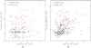 |
Fig. 4 Column density of C18O vs. the peak flux densities of protostellar (red triangles) and prestellar (black triangles) cores at (a) 70 μm and (b) 250 μm selected from Könyves et al. (2015). The number of prestellar cores in panel a is less than the total number because some have no 70 μm flux. A clear separation is found between prestellar and protostellar cores in panel a (shown with a dotted line). Panel b: increasing trend of the 250 μm flux density with the C18O column density suggesting that star formation is more advanced at higher column densities and that an increasing volume is affected by the ongoing star formation. |
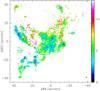 |
Fig. 5 Map of the abundance ratio |


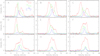 |
Fig. 6 Averaged spectra of 12CO(1−0) (red), 13CO(1−0) (green), and C18O(1−0) (blue) emission at the selected regions from Fig. 5. The name of the selected region is presented in the top-left corner of each panel. |
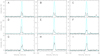 |
Fig. 7 Examples of the 12CO self-absorption correction. The blue dashed line presents the best single Gaussian fitting for the original 12CO profile using the remaining wings of the emission line. The name of the selected region is presented in the top-left corner of each panel. |
Integrated properties of the distinct regions.
3.8 Correlating the infrared and photo-dissociation data
The heating of the interstellar dust by the star formation processes first results in 250 μm infrared emission and at a later stage produces 70 μm emission (e.g. Bendo et al. 2015). Therefore, the 70/250 μm ratio could be an indicator of the evolutionary age of the star formation process and the state of the interstellar dust. On the other hand, photo-dissociation is clearly a time-dependent effect resulting from the UV exposure of the molecular gas and the photo-dissociation rate also reflects the evolutionary age of the selected distinct regions.
The peak flux density at the prestellar and protostellar cores at a wavelength of 70 μm versus the column density of C18O(1−0) reveals a separationbetween the prestellar and protostellar core distributions (Fig. 4a). The variation of the 250 μm emission data suggests a flux density increase at higher C18O column densities, such that the more intense star formation is able to heat a larger volume of the surrounding dust, which is also time dependent (Fig. 4b). Figure 8 displays the column density of C18O versus the peak flux density ratio F70μm∕F250μm of protostellar and prestellar cores. Excluding some improperly distributed stellar cores, most evolved protostellar cores are in the upper part, and the youthfulprestellar cores are in the lower part in the diagram. However, the dividing line between the flux ratio decreases with an increasing C18O column density because at higher C18O columns the star formation has time and energy to heat larger volumes of dust. The flux ratio F70μm∕F250μm diagram confirms that the C18O column density is related to the evolutionary age of the cores.
The abundance ratio of  /
/ for the prestellar and protostellar locations plotted against the C18O column density shows a similar distribution for prestellar and protostellar cores, which indicates that the effects of photodissociation only depend on the presence of star formation at this C18O column density (Fig. 9). The
  /
/ abundance ratio decreases with increasing C18O column density indicating an enhancement of C18O in the interstellar medium. The strong variation of the abundance ratio with the C18O column density shows that the more massive and fragmented star formation has a strong effect on the surrounding area.
The actual mass of the star formation region containing young stellar objects plays a critical role in distinguishing between evolutionary paths and their timescales. In order to depict the evolutionary path of star formation regions in the AMC, the original mass estimated from the reconstructed 12CO emission line in the nine selected regions is plotted against the 70 μm flux density in Fig. 10a. This diagram shows that the regions lie along a string of points indicating five stages of evolution. Region D, next to the W 40 HII, belongs to the oldest evolutionary stage with the highest amount of photo-dissociated mass (∽ 74 M⊙), and with the highest 70 μm flux density. The regions B and E form the next oldest stage of evolution, where region B is the Serpens South region and region E is a filament located southeast of the W 40 HII. Region E has lost more mass to photo-dissociation than region B. Regions G, F, A, and C resemble regions of an earlier stage of evolution, where region C has lost a little more mass than the others because it is larger. The youngest star formation region H is just starting to show up in 70 μm images. Region I is the youngest region located on the outskirts of the cloud; it does not yet show any 70 μm flux and has the least estimated mass of all the selected regions.
As UV radiation selectively dissociates less-abundant CO isotopologues more effectively than more-abundant ones (van Dishoeck & Black 1988; Liszt 2007; Shimajiri et al. 2014) the ratio  is equivalent to the dissociation rate of the C 18O. A similar evolutionary sequence is found when plotting the ratio
  against the flux ratio F70μm∕F250μm of the selected regions in Fig. 10b. However, the mid-range evolutionary regions cluster together in this case, possibly because of inaccuracies in estimating the abundance ratio. The two diagrams of Fig. 10 present the original mass, and the rate of photodissociation combined with the infrared properties are useful to determine the evolutionary age of the star-forming regions.
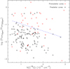 |
Fig. 8 Column density of C18O vs. the peak fluxdensity ratio of the bandwidth of 70 and 250 μm of the protostellar (red triangles) and prestellar (black triangles) cores selected from Könyves et al. (2015). The dotted line indicates the dividing line between prestellar and protostellar cores and shows the gradual change of the ratio. |
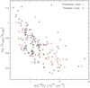 |
Fig. 9 Column density of C18O vs. the abundance ratio |


3.9 Uncertainties on the abundance ratio X13CO/XC18O introduced by the excitation temperature and the beam-filling factor
C18O and 13CO beam-filling factors were assumed to be unity when estimating their column densities and optical depths in Sect. 3.4. Also, the excitation temperatures (Tex) for all three lines C18O, 13CO, and 12CO were presumed to have the same values, as derived from the optically thick line 12CO.
Calculation of the beam-filling factor is obtained through Eq. (8):
 (8)
(8)
where θbeam is the beam size and θs is source diameter. The 13CO and C18O data have an effective beam size of 60′′ corresponding to 0.124 pc at the distance of the AMC. C18O emission is deemed as a tracer of dense cores, filaments, and clumps. In comparison, the 13CO emission will additionally trace extended components which could be seen via integrated intensity maps (Shimajiri et al. 2014). The nearest low-mass star forming region observations toward the Taurus cloud traced via C18O have dense cores of 0.1 pc in diameter (Onishi et al. 1996). Moreover, the constant encounter of parsec-scale filaments with narrow widths of typically 0.1 pc within molecular clouds were discovered through Herschel micrometre emission observations (Arzoumanian et al. 2011; Palmeirim et al. 2013). This infers that traced 13CO and C18O sources will have dimensions of over 0.1 pc. Assuming θsource > 0.1 pc and θbeam = 0.124 pc, we anticipate the beam to exceed 0.6. The affects of the beam filling factor on the abundance ratios and column densities are summarised in Table 2. The column density values for both C18O and 13CO are higher with the assumption of ϕ = 0.6 compared to those when ϕ = 1 is assumed. Nevertheless, the beam filling factor corrections play a insignificant role in estimating  /
/ .
.
As 12CO emission is affected by self-absorption, C18O and 13CO column densities are affected by underestimates of Tex from the 12CO data. The influence of uncertainties related to the excitation temperature on the derived physical properties is investigated assuming Tex (C18O) = 20 K and  = 30 K. This is further illustrated in Table 2. The column density values for both 13CO and C18O with the assumption of Tex(C18O) = 20 K and
  = 30 K increase compared with those where
  = Tex(C18O) =
  . However, the range of
  /
/ with Tex(C18O) = 20 K and
  = 30 K is slightly narrower compared with those of
  = Tex(C18O) =
  . The higher abundance ratios (
 /
/ ) in all assumptions correspond to region D next to the W 40 HII.
When including uncertainties on excitation temperatures and beam filling factors of 13CO and C18O, we are convinced that the abundance ratio  /
/ is lower towards more actively star-forming regions in the AMC, with the exception of one region showing a particularly high abundance ratio (next to the W 40 HII).
3.10 Comparison with H2CO absorption
As regions B, D, and G have been identified as distinct star formation regions in the H2 CO absorption map of the AMC, a comparison may be made between the C18O distribution and the H2CO absorption (Komesh et al. 2019). Figure 11 shows a map of the C 18O(1−0) integrated intensity superposed on the integrated absorption contours of H2 CO. The C18O(1−0) and H2 CO data were smoothed to the same effective resolution and cell size of 10′ and 2.5′, respectively. The outer edges of the C18O emission (∽0.7 K km s−1) follow the lower contours of H2CO (∽0.4 K km s−1) and the contours encompass all identified star formation regions in the C18O data. The stronger C18O emission surrounding W 40 does not correspond to the H2CO absorption, because the H2CO absorption is related to the radio continuum of the H II region while the enhanced C18O emission results from heating by the H II region. The C18O emission map at Serpens South shows several elongated structures that only partially follow the H2 CO absorption structure. On a large scale the H2CO absorption structure is similar to the C18O(1−0) distribution but does not identify all active star formation regions.
4 Conclusion
Archival data of wide-field OTF observations of 12CO, 13CO, and C18O (J = 1–0) emission lines of the AMC were used to study star formation activity in the region and its influence on the surrounding areas. In the AMC, the distribution of protostellar and prestellar cores are a first indication of the locations of active star formation and their distribution is well correlated with the highest column densities within the structure of the extended C 18O(1−0) emission. This extended star formation structure is also found within the contours of the H2 CO absorption against the continuum of the region.
The abundance ratio  /
/ in our observations confirms that selective FUV photodissociation of C18O indeed occurs. As photo-dissociation results from FUV exposure of the surrounding molecular gas, photo-dissociation is a time-dependent process that may serve as an indicator of the evolutionary age of star formation. This effect is confirmed by a strong reduction in the abundance ratio
  /
/ with increasing C18O column density.
To evaluate how the beam filling factor affects the  /
/ abundance ratio, we consider the beam filling factor to exceed 0.6 for both C18O and 13CO gas. The abundance ratio
  /
/ distribution in the AMC was found to be similar even after the consideration of uncertainties on the beam filling factor. The beam filling factor corrections play a insignificant role in estimating
  /
/ .
.
As the 12CO emission is affected by self-absorption, C18O and 13CO column densities are effected by underestimates of Tex (3.6–23.6 K)from the 12CO data. To study the affects of uncertainties related to excitation temperature measurements on derived physical properties,we used the assumption of Tex(C18O) = 20 K and  = 30 K. Even if we consider higher excitation temperatures for the 13CO and C18O lines, we come to the same conclusion, namely that with the exception of one region of high abundance ratio (next to the W 40 HII), the abundance ratio
  /
/ is lower toward more actively star forming regions in the AMC.
The FUV radiation field originating at the location of massive and even fragmented star formation will also heat the surrounding molecular regions. This heating process will increasingly result in 250 μm FIR emission and also 70 μm emission after a certain evolutionary period. The 70/250 μm flux density ratio can therefore also serve as an evolutionary age indicator and this ratio is indeed found to vary with the C18O column density.
We tested these evolutionary indicators with a number of selected star-formation and non-star-formation regions for which we estimated the dissociation rate using the ratio  . We find a clear sequence for these selected regions when correlating the 70 μm flux density with the estimated original mass of the regions. Similarly, we find a clear sequence when correlating the 70/250 μm flux density ratio with the estimated photo-dissociation rate. These observed parameters of the molecular medium surrounding the star formation provide a measure of the intensity of the star formation process as well as a measure of the evolutionary age of the region.
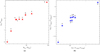 |
Fig. 10 (a) Mass-corrected self-absorption vs. 70 μm flux, and (b) the ratio |
Column densities and abundance ratio  /
/ of 13CO and C 18O.
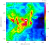 |
Fig. 11 Map of the C18O(1−0) integrated intensity superposed on the contours of H2CO absorption toward the AMC. The C18O(1−0) and H2 CO data were smoothed to the same effective resolution and cell size of 10′ and 2.5′, respectively. Contour levels of the H2CO intensity map are −0.4 to − 1.8 in steps of −0.15 K km s−1. The white circle presents the location of the W 40 H II region (radius ∽3′) and the black circle in the bottom-right illustrates the resolution of 10′. |
Acknowledgements
This work was sponsored by CAS-TWAS President’s Fellowship for International Doctoral Students, and The National Natural Science foundation of China under grants 11433008, 11973076, 11703074, 11703073 and 11603063. W.A.B. has been funded by Chinese Academy of Sciences President’s International Fellowship Initiative under grants 2021VMA0008 and 2019VMA0040. Collaboration between Z.R. and the main author was supported by the University of Malaya grant UMRG FG033-017AFR. This publication makes use of data products from the 13.7 m telescope of the Qinghai observation station of the Purple Mountain Observatory and the millimeter wave radio astronomy database, and the data from the Herschel Gould Belt survey (HGBS) project (http://gouldbelt-herschel.cea.fr). The HGBS is a Herschel Key Programme jointly carried out by SPIRE Specialist Astronomy Group 3 (SAG 3), scientists of several institutes in the PACS Consortium (CEA Saclay, INAF-IFSI Rome and INAF-Arcetri, KU Leuven, MPIA Heidelberg), and scientists of the Herschel Science Center (HSC).
References
- Anders, E., & Grevesse, N. 1989, Geochim. Cosmochim. Acta, 53, 197 [Google Scholar]
- André, P., Men’shchikov, A., Bontemps, S., et al. 2010, A&A, 518, L102 [NASA ADS] [CrossRef] [EDP Sciences] [Google Scholar]
- Arzoumanian, D., André, P., Didelon, P., et al. 2011, A&A, 529, L6 [Google Scholar]
- Bendo, G. J., Baes, M., Bianchi, S., et al. 2015, MNRAS, 448, 135 [NASA ADS] [CrossRef] [Google Scholar]
- Bontemps, S., André, P., Könyves, V., et al. 2010, A&A, 518, L85 [NASA ADS] [CrossRef] [EDP Sciences] [Google Scholar]
- Glassgold, A. E., Huggins, P. J., & Langer, W. D. 1985, ApJ, 290, 615 [NASA ADS] [CrossRef] [Google Scholar]
- Gutermuth, R. A., Bourke, T. L., Allen, L. E., et al. 2008, ApJ, 673, L151 [NASA ADS] [CrossRef] [Google Scholar]
- Kawamura, A., Onishi, T., Yonekura, Y., et al. 1998, ApJS, 117, 387 [NASA ADS] [CrossRef] [Google Scholar]
- Kim, S.-J., Kim, H.-D., Lee, Y., et al. 2006, ApJS, 162, 161 [NASA ADS] [CrossRef] [Google Scholar]
- Komesh, T., Esimbek, J., Baan, W., et al. 2019, ApJ, 874, 172 [CrossRef] [Google Scholar]
- Kong, S., Lada, C. J., Lada, E. A., et al. 2015, ApJ, 805, 58 [NASA ADS] [CrossRef] [Google Scholar]
- Könyves, V., André, P., Men’shchikov, A., et al. 2015, A&A, 584, A91 [NASA ADS] [CrossRef] [EDP Sciences] [Google Scholar]
- Lada, C. J., Lada, E. A., Clemens, D. P., et al. 1994, ApJ, 429, 694 [NASA ADS] [CrossRef] [Google Scholar]
- Liszt, H. S. 2007, A&A, 476, 291 [NASA ADS] [CrossRef] [EDP Sciences] [Google Scholar]
- Lin, S.-J., Shimajiri, Y., Hara, C., et al. 2016, ApJ, 826, 193 [NASA ADS] [CrossRef] [Google Scholar]
- Onishi, T., Mizuno, A., Kawamura, A., et al. 1996, ApJ, 465, 815 [NASA ADS] [CrossRef] [Google Scholar]
- Ortiz-León, G. N., Dzib, S. A., Kounkel, M. A., et al. 2017, ApJ, 834, 143 [NASA ADS] [CrossRef] [Google Scholar]
- Palmeirim, P., André, P., Kirk, J., et al. 2013, A&A, 550, A38 [NASA ADS] [CrossRef] [EDP Sciences] [Google Scholar]
- Pineda, J. L., Goldsmith, P. F., Chapman, N., et al. 2010, ApJ, 721, 686 [NASA ADS] [CrossRef] [Google Scholar]
- Shimajiri, Y., Kitamura, Y., Saito, M., et al. 2014, A&A, 564, A68 [NASA ADS] [CrossRef] [EDP Sciences] [Google Scholar]
- Smith, J., Bentley, A., Castelaz, M., et al. 1985, ApJ, 291, 571 [NASA ADS] [CrossRef] [Google Scholar]
- Strong, A. W., Bloemen, J. B. G. M., Dame, T. M., et al. 1988, A&A, 207, 1 [NASA ADS] [Google Scholar]
- Su, Y., Yang, J., Yan, Q.-Z., et al. 2020, ApJ, 893, 91 [CrossRef] [Google Scholar]
- Tan, B.-K., Leech, J., Rigopoulou, D., et al. 2013, MNRAS, 436, 921 [NASA ADS] [CrossRef] [Google Scholar]
- Tielens, A. G. G. M., & Hollenbach, D. 1985, ApJ, 291, 722 [NASA ADS] [CrossRef] [Google Scholar]
- Ulich, B. L., & Haas, R. W. 1976, ApJS, 30, 247 [NASA ADS] [CrossRef] [Google Scholar]
- van Dishoeck, E. F., & Black, J. H. 1988, ApJ, 334, 771 [NASA ADS] [CrossRef] [Google Scholar]
- Yurimoto, H., & Kuramoto, K. 2004, Science, 305, 1763 [NASA ADS] [CrossRef] [PubMed] [Google Scholar]
All Tables
All Figures
|
Fig. 1 Aquila maps of the intensities of (a) 12CO (1−0), (b) 13CO (1−0), and (c) C 18O (1−0) integrated from 2 to 12 km s−1. White filled circles in the bottom-right corner of each panel illustrate the beam size of 60′′. (d) The Herschel 250 μm image (the beam size is 18.2′′) taken from André et al. (2010). The circle and star mark the locations of the W 40 H II region (radius ∽ 3′) and the Serpens South, respectively. |
| In the text | |
|
Fig. 2 Map of the column density of C18O(1− 0). The black stars and triangles present the locations of protostellar and prestellar cores, respectively. The coordinates of the protostellar and prestellar cores were taken from Könyves et al. (2015). The black circle marks the location of the W 40 H II region (radius ∽ 3′) and the black filled circle in the bottom-right corner illustrates the beam size of 60′′. The clippinglevel for the 13CO and C18O data corresponds to a signal-to-noise ratio greater than five. Gaussian fitting to each pixel was done. |
| In the text | |
|
Fig. 3 Histograms of the distributions of (a) the number of pixels with certain column density of C18O(1−0), (b) the number of prestellar cores with this density, and (c) the protostellar cores with this column density. The prestellar and protostellar sources clearly sample the larger C18O column densities. |
| In the text | |
|
Fig. 4 Column density of C18O vs. the peak flux densities of protostellar (red triangles) and prestellar (black triangles) cores at (a) 70 μm and (b) 250 μm selected from Könyves et al. (2015). The number of prestellar cores in panel a is less than the total number because some have no 70 μm flux. A clear separation is found between prestellar and protostellar cores in panel a (shown with a dotted line). Panel b: increasing trend of the 250 μm flux density with the C18O column density suggesting that star formation is more advanced at higher column densities and that an increasing volume is affected by the ongoing star formation. |
| In the text | |
|
Fig. 5 Map of the abundance ratio |
| In the text | |
|
Fig. 6 Averaged spectra of 12CO(1−0) (red), 13CO(1−0) (green), and C18O(1−0) (blue) emission at the selected regions from Fig. 5. The name of the selected region is presented in the top-left corner of each panel. |
| In the text | |
|
Fig. 7 Examples of the 12CO self-absorption correction. The blue dashed line presents the best single Gaussian fitting for the original 12CO profile using the remaining wings of the emission line. The name of the selected region is presented in the top-left corner of each panel. |
| In the text | |
|
Fig. 8 Column density of C18O vs. the peak fluxdensity ratio of the bandwidth of 70 and 250 μm of the protostellar (red triangles) and prestellar (black triangles) cores selected from Könyves et al. (2015). The dotted line indicates the dividing line between prestellar and protostellar cores and shows the gradual change of the ratio. |
| In the text | |
|
Fig. 9 Column density of C18O vs. the abundance ratio |
| In the text | |
|
Fig. 10 (a) Mass-corrected self-absorption vs. 70 μm flux, and (b) the ratio |
| In the text | |
|
Fig. 11 Map of the C18O(1−0) integrated intensity superposed on the contours of H2CO absorption toward the AMC. The C18O(1−0) and H2 CO data were smoothed to the same effective resolution and cell size of 10′ and 2.5′, respectively. Contour levels of the H2CO intensity map are −0.4 to − 1.8 in steps of −0.15 K km s−1. The white circle presents the location of the W 40 H II region (radius ∽3′) and the black circle in the bottom-right illustrates the resolution of 10′. |
| In the text | |
Current usage metrics show cumulative count of Article Views (full-text article views including HTML views, PDF and ePub downloads, according to the available data) and Abstracts Views on Vision4Press platform.
Data correspond to usage on the plateform after 2015. The current usage metrics is available 48-96 hours after online publication and is updated daily on week days.
Initial download of the metrics may take a while.