| Issue |
A&A
Volume 643, November 2020
|
|
|---|---|---|
| Article Number | A38 | |
| Number of page(s) | 9 | |
| Section | Planets and planetary systems | |
| DOI | https://doi.org/10.1051/0004-6361/202038567 | |
| Published online | 29 October 2020 | |
Physical and dynamical characterization of the Euphrosyne asteroid family
1
European Southern Observatory (ESO), Alonso de Cordova 3107,
1900
Casilla Vitacura,
Santiago, Chile
e-mail: This email address is being protected from spambots. You need JavaScript enabled to view it.
2
Institute of Astronomy, Faculty of Mathematics and Physics, Charles University,
V Holešovičkách 2,
18000
Prague, Czech Republic
3
Institute for Astronomy, University of Hawaii,
34‘Õhi‘a Kũ St.
Pukalani,
USA
4
Jet Propulsion Laboratory, California Institute of Technology,
4800 Oak Grove Drive,
Pasadena,
CA
91109, USA
5
Department of Physics and Astronomy, University of Hawaii at Hilo,
481 W Lanikaula St,
Hilo, USA
Received:
2
June
2020
Accepted:
19
August
2020
Abstract
Aims. The Euphrosyne asteroid family occupies a unique zone in orbital element space around 3.15 au and may be an important source of the low-albedo near-Earth objects. The parent body of this family may have been one of the planetesimals that delivered water and organic materials onto the growing terrestrial planets. We aim to characterize the compositional properties as well as the dynamical properties of the family.
Methods. We performed a systematic study to characterize the physical properties of the Euphrosyne family members via low-resolution spectroscopy using the NASA Infrared Telescope Facility. In addition, we performed smoothed-particle hydrodynamics (SPH) simulations and N-body simulations to investigate the collisional origin, determine a realistic velocity field, study the orbital evolution, and constrain the age of the Euphrosyne family.
Results. Our spectroscopy survey shows that the family members exhibit a tight taxonomic distribution, suggesting a homogeneous composition of the parent body. Our SPH simulations are consistent with the Euphrosyne family having formed via a reaccumulation process instead of a cratering event. Finally, our N-body simulations indicate that the age of the family is 280−80+180 Myr, which is younger than previous estimates.
Key words: minor planets, asteroids: general / minor planets, asteroids: individual: (31) Euphrosyne / methods: observational / methods: numerical
© ESO 2020
1 Introduction
The asteroid belt is a living relic leftover from the planet-formation epoch of our Solar System. However, traces of primordial conditions have been gradually obscured by ongoing collisional and dynamical evolution processes (Bottke et al. 2015). Physical observations and dynamical models of the main asteroid belt allow us to constrain the planet-formation scenarios and gain understanding of how the main belt reached its current state (Bottke et al. 2015). Asteroid families, products of collisional events, serve as a powerful tool to investigate the collisional and dynamical evolution of the asteroid belt (Milani et al. 2014).
Among a few large low-albedo families, the Euphrosyne asteroid family uniquely occupies a highly inclined region in the outer main belt, bisected by the ν6 secular resonance (Carruba et al. 2014). Asteroids in circulating orbits and aligned librating states of the ν6 resonance are unstable on short timescales because of close encounters with planets. In contrast, asteroids in anti-aligned librating states of the ν6 resonance, such as the Euphrosyne family members, may be stable on timescales up to hundreds of millions of years (Machuca & Carruba 2012; Carruba et al. 2014). The Euphrosyne family is one of the largest families, with more than 2600 associated members and may be an important contributor to the low-albedo subpopulations of the near-Earth objects (Mainzer et al. 2011; Masiero et al. 2015). Given the low number density in the phase space for proper inclination sinip > 0.3, the remarkably large number of members in the Euphrosyne family may be due to the relatively high collisional velocities (Milani et al. 2014) in the Euphrosyne region. Dynamical analysis suggests that the cratering event that formed the Euphrosyne family most likely occurred between 560 and 1160 Myr ago (Carruba et al. 2014).
Using the method introduced by DeMeo & Carry (2013), Carruba et al. (2014) analyzed the photometric data from the Sloan Digital Sky Survey (SDSS) Moving Object Catalog to investigate the taxonomical distribution in the Euphrosyne region. Similar to other regions in the outer belt, the Euphrosyne region is overwhelmingly dominated by primitive materials, with ~68% C-type, 20% X-type, and 7% B-type asteroids. The family shows an average albedo of pV = 0.056 ± 0.016, with only 1.5% of members having an albedo >0.1 (Masiero et al. 2013).
In this paper, we present the physical and dynamical characterization of the properties of the Euphrosyne family. We obtain low-resolution spectra of 19 suggested family members with NASA Infrared Telescope Facility (IRTF)/SpeX (Sect. 3). We identify members associated with this family using the hierarchical clustering method and construct the size–frequency distribution of this family (Sect. 4). We further constrain the family-forming event by smoothed-particle hydrodynamics (SPH) simulations (Sect. 5), study the orbital evolution of the family, and constrain its age using N-body simulations (Sect. 6). An additional discussion related to the observed shape of (31) Euphrosyne using disk-resolved images obtained with the Very Large Telescope (VLT) can be found in Yang et al. (2020).
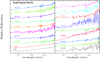 |
Fig. 1 Relative reflectance spectra of the Euphrosyne family members. All the spectra are normalized at 1.1 μm and are offset vertically for clarification. |
2 Observations and data reduction
The near infrared (NIR) spectra of the Euphrosyne family members were obtained using the IRTF 3-m telescope atop Mauna Kea, Hawaii. The observed family members (n = 19), including (31) Euphrosyne, are selected based on the dynamical study of Novaković et al. (2011), targeting the best observables in terms of their brightness and on-sky placement. An upgraded medium-resolution 0.7–5.3 μm spectrograph (SpeX) was used, equipped with a Raytheon 1024 × 1024 InSb array that has a spatial scale of 0.′′ 10 pixel−1 (Rayner et al. 2003). The low-resolution prism mode was used to cover an overall wavelength range from 0.7 to 2.5 μm for all of our observations. We used a 0.8′′× 15′′ slit that provided an average spectral resolving power of ~130. To correct for strong telluric absorption features from atmospheric oxygen and water vapor, we used G2V-type stars that are close to the scientific target both in time and sky position as telluric calibration standard stars as well as solar analogs for computing relative reflectance spectra of scientific targets. During our observations, the slit was always oriented along the parallactic angle to minimize effects from differential atmospheric refraction. The SpeX data were reduced using the SpeXtool reduction pipeline (Cushing et al. 2004). A journal of observations is provided in Table 1.
Journal of the IRTF observations.
3 Spectroscopy survey of the Euphrosyne family
The reflectance spectra of the Euphrosyne family members are shown in Fig. 1. The physical properties of these asteroids are listed in Table 2. Our observations show that the family members exhibit neutral to slightly red spectral slopes in the NIR. We classified 17 family members for the first time using their NIR reflectance spectra from 0.80 to 2.45 μm based on the Bus-DeMeo (BD) taxonomic system (DeMeo et al. 2009). To classify these objects, we resampled and normalized all the spectra at 1.5 μm, which is free of intrinsic absorption features as well as atmospheric absorptions, and calculated χ2 difference between the asteroid spectrum and the mean spectrum of each taxonomy class taken from DeMeo et al. (2009). We compared our classification results with the results based on the principal component analysis performed with the Bus-DeMeo Taxonomy Classification Web tool1 and found that the two methods are consistent for most cases. Using the NIR-only spectra, the BD classification system returned unique classification for less than half of the family members. For members with non-unique taxonomic classifications, we list the two types with the lowest χ2 values in Table 2. The majority of the family members belong to the C-types, as shown in Fig. 2, indicating a homogeneous composition of the parent body for the Euphrosyne family. Our finding is consistent with the previous study using the SDSS data (Carruba et al. 2014).
Physical properties of studied Euphrosyne family members.
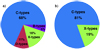 |
Fig. 2 Relative taxonomic distributions of the Euphrosyne family based on the BD taxonomic system: (a) with all the objects (n = 19); (b) with the interlopers (895, 66360, and 79478) removed (n = 16). |
3.1 Detection of 1-μm absorption feature
The largest member, asteroid 31, shows a broad but shallow absorption feature, centered near 1.0- μm; see Fig. 3. Such a rounded absorption feature near 1.0-μm has also been observed on other large C-type asteroids, e.g. (1) Ceres and (10) Hygiea (Takir & Emery 2012). Compared to the two larger asteroids, the absorption features of Euphrosyne, in both the 1- μm region and the 3-μm region, appear weaker in terms of the band depth.
We detected the broad 1-μm feature in 8 of the 19 objects. Among these eight asteroids, seven are C-types with one exception, which is 79478, a D-type based on its very red spectral slope. The band centers of these absorption features vary from 0.84 to 1.05 μm. It is well known that some silicates and hydrated minerals show a diagnostic absorption band around 1.0- μm, such as pyroxene, olivine, and magnetite. Magnetite is a product of aqueous alteration and has been detected on some B-type asteroids (Yang & Jewitt 2010) and on the dwarf planet Ceres (de Sanctis et al. 2015). To further explore the compositional origin of this absorption feature, we searched for spectral analogs for the Euphrosyme family members among meteorites and silicate minerals. We present the results in Sect. 3.2.
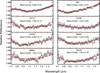 |
Fig. 3 Illustration of the profile of the 1-μm absorption band observed among the Euphrosyne family members. The reflectance spectra are shown as open triangles and the best-fit Gaussian models are shown as the red lines. |
3.2 Spectral analogs
We selected four asteroids that have high-quality spectra and are representative of the spectral diversity of the family for further analysis. We excluded 79478 from the spectral modeling because its spectrum is rather noisy beyond 1.5 μm. We combined the IRTF data with the available optical data to cover a wider range of wavelengths. We searched for spectral analogs for the Euphrosyne family among the collections of the RELAB spectral library (Hiroi et al. 2001) and the USGS spectral library (Survey et al. 2017).
As shown in Fig. 4, the shape of the absorption band of asteroid 31 is different from that of magnetite (shown in green), where the magnetite band has a narrower profile and the band center is at a longer wavelength. Instead, the round feature on 31 is similar to the 1.0-μm band of hedenbergite (shown in blue), which is an iron-rich end member of the pyroxene group. However, discrepancies are observed both at the shorter and the longer end of the spectra between the asteroid and hedenbergite. The best spectral match, from 0.9 to 2.5 μm, is a mixture of the Ivuna meteorite and the Murchison meteorite.
When combining with the optical spectrum, the difference between asteroid 31 and asteroid 895 in terms of the 1.0- μm feature appears more prominent. Compared to the feature of 31, the latter is broader with a band center at shorter wavelength and it cannot be fit with either carbonaceous meteorites or with olivine. Except for the wavelengths below 0.6- μm, the spectrum of hedenbergite fits the overall spectral profile of 895 adequately well including the 1.0 μm feature.
The spectrum of 16712 shows a marginal absorption feature between 0.7 and 1.5 μm, which can be fit with the heated Murchison or with the heated olivine spectrum. However, the optical colors of 16712 obtained by the SDSS (Ivezić et al. 2001) show a downturn below 0.7 μm, which is not observed in the olivine spectrum. A mixture of heated Murchison with a small amount of heated Ivuna fits the spectrum of 16712 better, especially when taking into account the optical part.
Among all the observed family members, asteroid 66360 is one of the reddest objects in the NIR and has the steepest spectral slope in the optical. The spectrum of 66360 is very different from those of C-type asteroids; instead it is more similar to D-type asteroids or Trojan asteroids. As suggested in Yang et al. (2013), the red Trojan asteroid spectra can be fitted with a mixture of fine-grained silicates and iron. The spectrum of metallic iron can fit the 66360 spectrum well but discrepancies were observed at wavelengths longwards of 1.5 μm. The similarity between the D-type asteroids and the Tagish Lake meteorite was previously noted by Hiroi et al. (2001). Consistently, we found the best spectral analog for 66360 is the Tagish Lake meteorite.
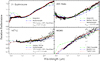 |
Fig. 4 Spectral analogs for the Euphrosyne family asteroids. The NIR spectra are indicated with plus symbols and the optical spectra are shown as open diamond symbols. The optical spectra of 31 and 895 are taken from the SMASSII survey (Bus & Binzel 2002) and the optical colors of 16712 and 66360 are taken from the SDSS-MOC4 catalog (Ivezić et al. 2001)following the method in DeMeo & Carry (2013). For three objects that show an absorption band in the 1-μm region, we present the wavelength coverage of the absorption band in the parenthesis. |
3.3 Possible interlopers
The second largest body in the Euphrosyne region, (895) Helio, is identified as a family member by Masiero et al. (2013) but is considered a dynamical interloper by Carruba et al. (2014). Our IRTF observation combined with the optical datareveal notable differences between Euphrosyne and Helio, especially at wavelengths shortwards of 1.0− μm. Also, spectral modeling shows that the best spectral analog for Helio is hedenbergite instead of carbonaceous meteorites, which are the best match for Euphrosyne as well as other Cb-type members. Therefore, 895 is likely an interloper. In addition, 66360 and 79478 have much redder spectral slopes than others, indicating that these objects have substantially different compositions, in contrast to other family members. Therefore, 66360 and 79478 are also likely interlopers.
 |
Fig. 5 Euphrosyne family in the space of proper elements (ap, ep, sinIp). Family members were determined using the HCM method, with the cutoff velocity vcut = 120 m s−1. Colors correspond to the geometric albedo pV (blue → yellow). Symbol sizes are proportional to diameters. Likely interlopers are also indicated (green crosses). There are numerous mean-motion resonances, namely J9/4, J11/5, J13/6, J15/7, J17/8, J2/1, as well as three-body resonances, 5J − 2S − 2, 7J − 2S − 3 (dotted or hatched) and the secular resonance ν6 (gray). The ellipses (orange) are constant velocity curves with respect to (31) Euphrosyne, equal to the escape velocity vesc ≐ 135 m s−1 from the parent body; they were only slightly shifted in eccentricity to 0.19 and in inclination to 0.45. Their shape is also determined by the true anomaly f, and the argument of perihelion ω at the time of breakup. We show the values f = 0°, 30°, 60° (top panel); ω + f = 30°, 60°, and 90° (bottom panel). |
4 Identification of the Euphrosyne family
In order to study the origin of the Euphrosyne family, we first identified the family members around (31) Euphrosyne with the hierarchical clustering method (HCM; Zappalà et al. 1995) and then removed interlopers based on the albedo data (Tedesco et al. 2002; Mainzer et al. 2016; Usui et al. 2011) and the color indices (Ivezić et al. 2002). The interloper removal procedure was not included in the membership identification in the previous study by Nesvorný et al. (2015). We also used more recent catalogs of proper elements (Knežević & Milani 2003) than previous works (Carruba et al. 2014; Nesvorný et al. 2015) to obtain a more reliable slope of the size–frequency distribution (SFD). We adopted the velocity cutoff vcut = 100–120 m s−1, the albedo range pV = 0–0.15, and the color index range a⋆ = −0.3 to 0.1. Depending on vcut, we identified 2603–2858 members and excluded 32–37 interlopers using their physical properties. We did not apply the (ap, H) criterion (Vokrouhlický et al. 2006) because the V-shape is not well defined due to the lack of intermediate-sized fragments. The distribution of family members in the space of proper elements is shown in Fig. 5.
The SFD of the family was constructed using known albedos. For objects with unknown albedos, we assumed pV = 0.056, corresponding to the median albedo of the family (Masiero et al. 2013). The slope is γ = − 4.7 ± 0.2 in the range of D = 7 to 30 km (see Fig. 6). A preliminary estimate of the parent body size is DPB = 280 km and the mass ratio of the largest remnant to the parent body MLR∕MPB = 0.960, which implies a cratering or reaccumulation event. For the density ρ = 1665 ± 242 kg m−3 (taken from Yang et al. 2020), this means the escape speed vesc = 135 m s−1, which is an important parameter for further modeling. The asteroid (895) Helio appears as an intermediate-size outlier. If we include 895 in the SFD, the parent body related parameters changes slightly to DPB = 289 km, MLR∕MPB = 0.876; we discuss its membership further in Sect. 5.
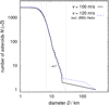 |
Fig. 6 Cumulative SFD of the Euphrosyne family for two values of the cutoff velocity, vcut = 100 and 120 m s−1. The latter one also includes (895) Helio, an intermediate-size object which is considered to be a possible interloper. In the interval of sizes D ∈ (7;25) km, the SFD can be fitted by a power-law with the slope − 4.7, with the uncertainty ±0.2. |
5 Collisional formation of the family
We coupled the observational data of the Euphrosyne family with hydrodynamical simulations to study the family-formation event. The simulations were used to constrain the impact parameters, such as the impact angle and the diameter of the impactor. We further estimated the initial speed distribution of the fragments. The simulations were performed using code OpenSPH (Sevecek 2019) with varying impact parameters. In these simulations, the impactor diameters ranged from dimg = 50 to 100 km and the impact angles from ϕimp = 15° to 60°. The impact speed was vimp = 5 km s−1 in all simulations, which roughly corresponds to the mean relative velocity in the main belt. We assumed a monolithic carbonaceous material with initial density ρ0 = 1600 kg m−3 for both thetarget and the impactor (consistent with the measurement presented in Yang et al. 2020).
The numerical model is described in detail in Ševeček et al. (2019). We modeled the family formation using a hybrid SPH/N-body approach. The impact, fragmentation, and initial reaccumulation were carried out using an SPH solver, which ran up to tfrag = 24 h. We then passed the results to a simple N-body solver with collision handling instead of hydrodynamics. The N-body reaccumulation phase ran for another treac = 10 days, at which point the resulting SFD was almost stationary.
During the fragmentation phase, we solved the continuity equation, the equation of motion, the energy equation, and the Hooke’s equation for the evolution of the stress tensor. For the equation of state, we used the Tillotson equation with the material parameters of basalt. To account for plasticity and fragmentation of the material, the von Mises rheology together with the Grady–Kippfragmentation model were used. This implies that completely fractured material is frictionless and essentially behaves likea fluid. To assess the plausibility of such a model for the studied impact, we also performed several simulations with the Drucker–Prager rheology, which – unlike the von Mises rheology – also includes cohesion and dry friction, meaning that even completely fractured material has non-negligible strength, determined by the coefficient μd of dry friction. The equations were integrated using a predictor–corrector scheme and the time-step was limited by the Courant–Friedrichs–Lewy (CFL) criterion with the Courant number C = 0.2. Figure 7 shows several snapshots of one of the performed SPH simulations.
At the end of the SPH phase, each SPH particle was converted into a sphere of equal volume and these spheres were used as inputs for an N-body solver. The N-body approach allowed us to use significantly larger time-steps, thus obtaining the final SFD much faster. We further merged collided fragments into larger spheres, provided their relative speed was lower than the escape speed vesc and the spin rate of the formed merger was lower than the critical spin rate ωcrit.
From the set of performed SPH/N-body simulations, we selected a few that are the most consistent with the SFD of the observed family. The synthetic SFDs as well as the observed SFD for reference are plotted in Fig. 8. Generally, impacts at low impact angles (ϕ ≃ 15°) tend to produce an intermediate-sized body originating from the antipode of the target. More oblique impacts (ϕ ≳ 30°) create no such fragments. This effect was previously recognized by Vernazza et al. (2020). However, even the largest intermediate body obtained in our simulations (D = 66 km) is still considerably smaller than asteroid (895) Helio with a diameter D ≃ 148 km (Carry 2012). Since no single fragment with similar size was created in the simulations, we conclude that (895) Helio is indeed an interloper, consistent with the spectroscopic arguments laid out above.
The lack of intermediate-sized bodies in the observed family suggests that the impact angle was likely in the mid-range values; a head-on impact would produce a large body which is not observed and a highly oblique impact would not have enough energy to eject the observed fragment mass. The probable size of the impactor is dimp ≃ 70–80 km. Naturally, a higher impact angle also implies a larger impactor to deliver the same kinetic energy into the target. Regardless of the impact angle, the SFDs of synthetic families have slightly steeper slopes compared to the observed SFD, suggesting the family has been modified by orbital evolution since its origin.
In addition to the SFDs, we plot the speed distribution of fragments in Fig. 9, since they were subsequently used as an input for the evolution simulations (Sect. 6). The distributions are similar in all performed simulations. The maximum value is approximately located at the escape speed vesc ≃ 109.7 m s−1 of the largest remnant. The impacts at larger impact angles generally produce flatter tails of the distribution, that is, faster fragments compared to head-on impacts.
6 Evolution and age of the family
Using the results of Sect. 5, we revisit here the question of the family age. For this purpose, we performed an N-body integration of a synthetic family. The integration was carried out with the symplectic Regularized Mixed Variable Symplectic 3 (RMVS3) scheme of the SWIFT package (Levison & Duncan 1994; Laskar & Robutel 2001). Our dynamical model contained (i) the gravitational influence of the Sun, six planets (from Earth to Neptune), and (31) Euphrosyne (M31 = 1.7 × 10¹⁹ kg, Yang et al. 2020); (ii) the Yarkovsky diurnal and seasonal effects (Vokrouhlický 1998; Vokrouhlický & Farinella 1999); and (iii) the YORP effect (Čapek & Vokrouhlický 2004) with collisional reorientations (Farinella et al. 1998) and random period changes for critically rotating asteroids, as described in Brož et al. (2011).
The synthetic family was initially comprised of ntp = 5712 test particles (i.e. twice as many as the observed family). Their initial orbits and parameters are described in detail in Appendix A. The family was integrated over 1 Gyr with a time-step of Δt = 1∕20 yr. We performed an on-line computation of proper orbital elements using the method discussed in Appendix A.
Figure 10 shows several snapshots of the evolving synthetic family in the (ap, ep) plane. At t = 50 Myr, the family is clearly insufficiently dispersed in ep. The asymmetry of the mean eccentricity between the inner and outer part of the family (Milani et al. 2019) is inherited from the mapping of the initial conditions (depending on the orbital configuration at the time of impact) to the proper element space (see Fig. A.2). Similarly, the considered ejection velocities were high enough to populate the region between 9:4 and 11:5 mean-motion resonances with Jupiter.
After the next ≃200 Myr of evolution,the family dynamically spreads due to combined effects of the Yarkovsky drift and resonant perturbations. Strong diffusion is observed close to the family center where the mean-motion resonances overlap with the ν6 secular resonance2 and the family members are located in the anti-aligned states (Machuca & Carruba 2012; Carruba et al. 2014; Huaman et al. 2018; Milani et al. 2019). For objects that are temporarily captured in the ν6 resonance, their ep can be pumped up significantly and subsequently be implanted into Jupiter-crossing, Mars-crossing, and even near-Earth orbits (Masiero et al. 2015). Therefore, including Mars and Earth together with other massive bodies in our simulations is essential to properly model the dynamical decay of the population. Comparing the synthetic and observed family, the distributions appear to be qualitatively the same except for the region at ap > 3.2 au, ep < 0.17 (which is underpopulated by synthetic asteroids), and the family halo (which is truncated from the observed population by the HCM).
At t = 600 Myr, the synthetic family seems to be strongly dispersed, especially towards low eccentricities. This suggests that the Euphrosyne family might be considerably younger than previous estimates (between 560 and 1160 Myr, Carruba et al. 2014).
To determine the age of the family, we analyzed our N-body simulation using the “black-box” method which was extensively described and tested in Brož & Morbidelli (2019). We split the intervals ap ∈ (3.03;3.258) au, ep ∈ (0;0.45), sin ip ∈ (0.41;0.475) into a grid of 10 × 9 × 3 boxes. In order to extend our statistical test to the family halo as well, we combined the observed family with all C-type asteroids in the given range of the orbital element space. The observed asteroids in the individual boxes were counted to obtain Nobs,i and we also determined the respective SFD.
For a given t, we randomly selected a subset of test particles from our synthetic family. The selection was always performed in given size bins to match the synthetic SFD with the observed SFD. The total number of test particles was exactly the same as the number of observed asteroids. Regarding the background population, we simply assumed that it is negligible because Euphrosyne is located in a highly inclined part of the main belt. The test particles were counted to obtain Nsyn,i. We constructed a statistical metric (Press et al. 1992):
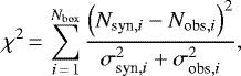 (1)
(1)
where Nbox is the number of boxes with nonzero N; with Poisson uncertainties  . This way we compare the distributions in the orbital element space.
Figure 11 shows the results of our χ2 test as a function of t. The global minimum at t = 281 Myr can be characterized by the ratio χ2∕Nbox = 2.4 which we consider low enough for the observed distributions to be equivalent. By calculating the 3- σ confidence levels of our test, we determined the age of the Euphrosyne family 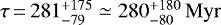 .
.
Figure 11 also shows the result of the χ2 test at t = 281 Myr in individual boxes (for a single selected section in inclinations). One can see that the largest difference between the observed and synthetic population surprisingly arises in the central region of the family.
 |
Fig. 7 Snapshots of the SPH simulation with the impactor diameter dimp = 70 km and the impact angle ϕimp = 30°. The images were captured at times t = 0, 4, 8, 12, 16, 20, 24 h after the impact. The color palette is given by the specific internal energy of the particles. |
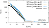 |
Fig. 8 Size–frequency distribution of three selected SPH simulations compared with the distribution of the observed Euphrosyne family. The diameter of a probable interloper (895) Helio is plotted as a black circle. |
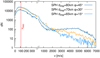 |
Fig. 9 Differential histogram of fragment speeds at the end of the reaccumulation phase. The velocities were evaluated in the reference frame of the largest remnant. |
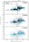 |
Fig. 10 Orbital evolution of the synthetic family (black circles) compared to the orbital distribution of the observed members of the actual Euphrosyne family (blue crosses) in the proper (ap, ep) plane. Dotted vertical lines are centers of several two-body and three-body mean-motion resonances located in the region of interest. The red dashed curve shows the approximate position of the ν6 secular resonance (adapted from Carruba et al. 2014; Milani et al. 2019). Individual snapshots, labeled with a corresponding integration time t, map the progress of our N-body simulation. They depict a compact family, the “best-fit” solution, and a dynamically dispersed family. |
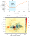 |
Fig. 11 Top: χ2 metric (orange curve) as a function of the simulation time t. The thick dashed line shows the evolution of Nbox, and the thin dashed lines are 1-σ and 3- σ confidence levels, the latter of which determines the interval of relevant ages of the family (light blue rectangle). The minimal ratio χ2∕Nbox is attained at t = 281 Myr. Bottom: a box-by-box map of the χ2 values at t = 281 Myr. The displayed (ap, ep) plane corresponds to the inclination range sinip ∈ (0.43;0.453). Black points and blue crosses are synthetic and observed asteroids, respectively. |
7 Discussion
In the NIR, the spectra of the Euphrosyne family members resemble those of the carbonaceous chondrite meteorites, and in particular, the CI and CM chondrites. Takir et al. (2015) report that CM and CI chondrites are possible meteorite analogs for asteroids with the sharp 3- μm features but do not match the rounded 3-μm feature observed on outer belt asteroids including (52) Europa and (31) Euphrosyne. In addition, recent studies at longer wavelengths show that the spectra of heated carbonaceous chondrites failed to fit the spectra of the C-type asteroids in the mid-infrared (Vernazza et al. 2015, 2017). The emission features in the 10- μm region of large asteroids can be reproduced using interplanetary dust particles (IDPs, Vernazza et al. 2015, 2017) or fine grained silicates entrained in a transparent matrix (Emery et al. 2006; Yang et al. 2013). At present, there is no natural material or synthetic mixture that can simultaneously fit both the NIR and the mid-IR spectra of primitive asteroids to a satisfactorily level. In order to gain a deeper and more comprehensive understanding of the intrinsic composition of an object, it is important to obtain observations over a wide range of wavelength coverage. To date, the thermal properties of intermediate and small asteroids remain largely unknown. The James Webb Space Telescope will be launched in 2021, which will offer an unprecedented opportunity to study small asteroids (Rivkin et al. 2016), such as the Euphrosyne family members in the 3- μm region and beyond.
The properties of the Euphrosyne family and our SPH simulations indicate that the family formed via a reaccumulative event. This means that the original shape of the parent body as well as the impact crater were not preserved, which is in agreement with AO observations (see the related discussion in Yang et al. 2020). Moreover, our orbital evolution model indicates that the age of the Euphrosyne family is τ ≃ 280 Myr. This is substantially younger than the previous estimates (Carruba et al. 2014) which were based on the evolution of the size–frequency distribution (with the assumed initial cumulative slope of − 3.8). The main goal of the previous work by Carruba et al. (2014) was to check the effect of the ν6 secular resonance on the size distribution of the family and on its evolution. Therefore, several simplified assumptions were used, such as the value of the initial cumulative slope and the assumption that secular dynamics dominated the evolution of the size distribution. In this paper, our model adopts a more realistic velocity field (with velocities of the order of vesc) than the previous assumption. The dynamical age is then constrained by the observed distribution of proper semimajor axis and eccentricity. We consider our estimate robust because the density of (31) Euphrosyne is well constrained (Yang et al. 2020) and the remaining uncertainty is solely related to possible porosity of smaller family members.
As discussed in Yang et al. (2020), a large fraction of water ice is needed to account for the low bulk density of (31) Euphrosyne. One problem that needs to be addressed is the survival of the water ice through the fragmentation and reaccumulation processes. Wakita & Genda (2019) studied the status of hydrous minerals in large planetesimals during collisional processes and pointed out that an oblique impact may enhance the effect of frictional heating because the leading side of the impact point can experience strong shear. Given the large size of the impactor and the impact velocity of 5 km s−1, it is inevitable that at least part of the original water ice was heated up and vaporized during the impact. For the surviving icy fragments, the lifetime of the exposed water ice depends on the impurity of the ice grains. The semi-major axis of the orbit of (31) Euphrosyne is 3.15 au. At this heliocentric distance, the lifetime of 10 μm-sized dirty icy grains is about a day (105 s, Beer et al. 2006). In contrast, μm-sized pure water ice grains can remain in solid form for over 1 Myr (Beer et al. 2006). Since the excavated water ice is from the interior of the parent body, it is likely to be free of impurities as observed in the ejecta of 9P/Temple 1 by Deep Impact (Sunshine et al. 2007). If a fraction of the original water ice could survive the impact heating, then it would easily remain solid during the reaccumulation phase.
In this paper, our SPH simulations only deal with rocky materials without adding an ice component. For future work, we will model SPH particles that are mixtures of basaltic material and water ice to check how much of the original water ice could be vaporized during the impact. In this model, we will also add radiative cooling to study if we can retain enough ice post-impact. If no water ice can be retained, then we have to consider alternatives for the low density of (31) Euphrosyne, such as the possibility that the majority of the disrupted fragments eventually reaccumulate into a rubble pile as suggested in Arakawa (1999) or that the parent body of the Euphrosyne family was a rubble pile to begin with Benavidez et al. (2018).
8 Conclusions
In this paper, we present the characterization of the physical as well as the dynamical properties of the Euphrosyne family. Our main findings are briefly summarized as follows:
- 1.
the spectroscopy survey of 16 family members shows that the family has a tight distribution of the spectral slopes, suggesting a homogeneous composition of the parent body;
- 2.
using a more realistic initial velocity field and the observed distribution of proper elements, our N-body simulations find the age of the Euphrosyne family to be τ =
 ;
; - 3.
the SPH simulations show that the family formed via a recent violent impact, in which the parent body was fragmented and subsequently reaccumulated into a spherical body.
This work is closely related to the ESO Large Program that is surveying large asteroids (ID: 199.C-0074, PI: Vernazza). We emphasize the need for a re-interpretation of asteroid-family models in the context of new adaptive-optics observations.
Acknowledgements
B.Y. and H.K. are visiting Astronomers at the Infrared Telescope Facility, which is operated by the University of Hawaii under contract NNH14CK55B with the National Aeronautics and Space Administration. This work has been supported by the Czech Science Foundation through grant 18-09470S (J. Hanuš, J. Ďurech, O. Chrenko, P. Ševeček) and by the Charles University Research program No. UNCE/SCI/023. M.B. was supported by the Czech Science Foundation grant 18-04514J. Computational resources were supplied by the Ministry of Education, Youth and Sports of the Czech Republic under the projects CESNET (LM2015042) and IT4Innovations National Supercomputing Centre (LM2015070).
Appendix A: Technical details of the N-body simulation
For the sake of completeness, we provide some details regarding our dynamical model which is used in Sect. 6 to derive the family age.
A.1 Computation of proper elements
In order to compute the proper orbital eccentricity ep and inclination ip, we usually apply the frequency-modified Fourier transform of Šidlichovský & Nesvorný (1996). However, we realized in our preparatory integrations that the method fails for some asteroids in the vicinity of overlapping resonances. These asteroids exhibited a splitting of the maximum of the power spectrum in g and s frequencies and then it became difficult to find a unique and time-stable solution for such cases.
Therefore, we replaced our routines for computation of proper elements with the approach of Knežević & Milani (2000). We proceeded as follows:
- (i)
we filtered the time series of osculating orbital elements by a sequence of digital low-pass filters (Quinn et al. 1991) to suppress fast oscillations with periods shorter than 1500 kyr;
- (ii)
we removed secular planetary forced terms from filtered equinoctal elements k = ecosϖ, h = esinϖ and q = sini∕2cosΩ, p = sini∕2sinΩ;
- (iii)
we translated the oscillating phase angles ϖ and Ω into linearized time series by adding multiples of 2π; and
- (iv)
we resampled the equinoctal elements into unequally spaced datasets (k(ϖ), h(ϖ)) and (q(Ω), p(Ω)) in which we searched for the amplitude of the Fourier mode with period 2π (see Ferraz-Mello 1981), thus obtaining the proper elements ep and sinip∕2, respectively. For the purposes of an off-line analysis, all proper elements (including ap) were further smoothed out by a running average with a window range of 1 Myr.
A.2 Initial conditions and parameters
Initial orbital data of planets were taken from the JPL DE405 ephemeris and the osculating elements of (31) Euphrosyne were adapted from the AstOrb database (version October 2019), choosing JD = 2 458 700.5 as the initial time t0. We applied a barycentric correction and a conversion to the Laplace plane. To generate synthetic family members, we created a collisional swarm of ntp = 5712 test particles (i.e. twice the number of the observed family members, excluding (31) Euphrosyne). We placed a synthetic parent body on an osculating orbit a = 3.155 au, e = 0.145, i = 27.5°, ω + f = 160°, f = 30° and we assigned ejection velocities vej to individual test particles. We chose vej pseudo-randomly from a merged ejection field of one of our SPH simulations (Sect. 5), as shown in Fig. A.1, but we randomized the orientations of velocity vectors, thus obtaining an isotropic collisional cluster.
The diameters of synthetic asteroids were taken from the observed SFD: each D (except for (31) Euphrosyne) was randomly assigned to two test particles. Initial spins were chosen uniformly from the interval of periods P ∈(2;10) h. The thermal parameters were chosen as follows:
- (i)
the bulk and surface densities were set to the value derived for (31) Euphrosyne ρbulk = ρsurf = ρ31 = 1665 kg m−3 (Yang et al. 2020);
- (ii)
the Bondalbedo A = 0.015 and IR emissivity ϵ = 0.9 were both chosen based on in situ observations of primitive C-type asteroids (101955) Bennu (DellaGiustina et al. 2019) and (162173) Ryugu (Grott et al. 2019);
- (iii)
the thermal capacity C = 460 J kg−1 K−1 was calculated following Wada et al. (2018) and assuming the approximate sub-solar temperature of (31) Euphrosyne Tss ≈ 160 K; and
- (iv)
the conductivity was set to K = 0.01 W m−1 K−1. These parameters lead to the thermal inertia
 , which is comparable, for example, to the mean value observed for ~101 km-sized main-belt asteroids (Hanuš et al. 2018).
Figure A.2 shows the first record of the proper orbital elements which is closest to the initial state of the synthetic family. The early occurrence of the inner/outer asymmetry of the proper eccentricity ep is simply a result of the chosen impact geometry.
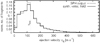 |
Fig. A.1 Histogram of ejection velocities vej used to generate initial orbits of test particles in our N-body simulation (solid line). The distribution was calculated by generating vej pseudo-randomly from an ejection velocity field of an SPH simulation (dashed line; see also Fig. 9). For reference, the dotted vertical line shows the escape velocity vesc from (31) Euphrosyne. |
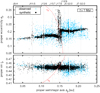 |
Fig. A.2 Orbital distribution of proper elements of the synthetic family (black circles) compared to the observed family (blue crosses). We plot the first record of proper elements obtained after 1 Myr of our N-body simulation –the distribution reflects the initial conditions. |
References
- Arakawa, M. 1999, Icarus, 142, 34 [NASA ADS] [CrossRef] [Google Scholar]
- Beer, E. H., Podolak, M., & Prialnik, D. 2006, Icarus, 180, 473 [NASA ADS] [CrossRef] [Google Scholar]
- Benavidez, P. G., Durda, D. D., Enke, B., et al. 2018, Icarus, 304, 143 [NASA ADS] [CrossRef] [Google Scholar]
- Bottke, W. F., Vokrouhlický, D., Walsh, K. J., et al. 2015, Icarus, 247, 191 [NASA ADS] [CrossRef] [Google Scholar]
- Brož, M., & Morbidelli, A. 2019, Icarus, 317, 434 [CrossRef] [Google Scholar]
- Brož, M., Vokrouhlický, D., Morbidelli, A., Nesvorný, D., & Bottke, W. F. 2011, MNRAS, 414, 2716 [NASA ADS] [CrossRef] [Google Scholar]
- Bus, S. J., & Binzel, R. P. 2002, Icarus, 158, 146 [NASA ADS] [CrossRef] [Google Scholar]
- Čapek, D., & Vokrouhlický, D. 2004, Icarus, 172, 526 [NASA ADS] [CrossRef] [Google Scholar]
- Carruba, V., Aljbaae, S., & Souami, D. 2014, ApJ, 792, 46 [NASA ADS] [CrossRef] [Google Scholar]
- Carry, B. 2012, Planet. Space Sci., 73, 98 [NASA ADS] [CrossRef] [Google Scholar]
- Cushing, M. C., Vacca, W. D., & Rayner, J. T. 2004, PASP, 116, 362 [NASA ADS] [CrossRef] [Google Scholar]
- de Sanctis, M. C., Ammannito, E., Raponi, A., et al. 2015, Nature, 528, 241 [NASA ADS] [CrossRef] [Google Scholar]
- DellaGiustina, D. N., Emery, J. P., Golish, D. R., et al. 2019, Nat. Astron., 3, 341 [Google Scholar]
- DeMeo, F. E., & Carry, B. 2013, Icarus, 226, 723 [NASA ADS] [CrossRef] [Google Scholar]
- DeMeo, F. E., Binzel, R. P., Slivan, S. M., & Bus, S. J. 2009, Icarus, 202, 160 [NASA ADS] [CrossRef] [Google Scholar]
- Emery, J. P., Cruikshank, D. P., & Van Cleve, J. 2006, Icarus, 182, 496 [NASA ADS] [CrossRef] [Google Scholar]
- Farinella, P., Vokrouhlický, D., & Hartmann, W. K. 1998, Icarus, 132, 378 [NASA ADS] [CrossRef] [Google Scholar]
- Ferraz-Mello, S. 1981, AJ, 86, 619 [NASA ADS] [CrossRef] [Google Scholar]
- Grott, M., Knollenberg, J., Hamm, M., et al. 2019, Nat. Astron., 3, 971 [NASA ADS] [CrossRef] [Google Scholar]
- Hanuš, J., Delbo’, M., Ďurech, J., & Alí-Lagoa, V. 2018, Icarus, 309, 297 [NASA ADS] [CrossRef] [Google Scholar]
- Hiroi, T., Zolensky, M. E., & Pieters, C. M. 2001, Science, 293, 2234 [NASA ADS] [CrossRef] [PubMed] [Google Scholar]
- Huaman, M., Roig, F., Carruba, V., Domingos, R. C., & Aljbaae, S. 2018, MNRAS, 481, 1707 [CrossRef] [Google Scholar]
- Ivezić, Ž., Tabachnik, S., Rafikov, R., et al. 2001, AJ, 122, 2749 [NASA ADS] [CrossRef] [Google Scholar]
- Ivezić, Ž., Lupton, R. H., Jurić, M., et al. 2002, AJ, 124, 2943 [NASA ADS] [CrossRef] [Google Scholar]
- Knežević, Z., & Milani, A. 2000, Celest. Mech. Dyn. Astron., 78, 17 [NASA ADS] [CrossRef] [Google Scholar]
- Knežević, Z., & Milani, A. 2003, A&A, 403, 1165 [NASA ADS] [CrossRef] [EDP Sciences] [Google Scholar]
- Laskar, J., & Robutel, P. 2001, Celest. Mech. Dyn. Astron., 80, 39 [NASA ADS] [CrossRef] [Google Scholar]
- Levison, H. F., & Duncan, M. J. 1994, Icarus, 108, 18 [NASA ADS] [CrossRef] [Google Scholar]
- Machuca, J. F., & Carruba, V. 2012, MNRAS, 420, 1779 [NASA ADS] [CrossRef] [Google Scholar]
- Mainzer, A., Bauer, J., Grav, T., et al. 2011, ApJ, 731, 53 [NASA ADS] [CrossRef] [Google Scholar]
- Mainzer, A. K., Bauer, J. M., Cutri, R. M., et al. 2016, NASA Planetary Data System, 247 [Google Scholar]
- Masiero, J. R., Mainzer, A. K., Bauer, J. M., et al. 2013, ApJ, 770, 7 [NASA ADS] [CrossRef] [Google Scholar]
- Masiero, J. R., Carruba, V., Mainzer, A., Bauer, J. M., & Nugent, C. 2015, ApJ, 809, 179 [NASA ADS] [CrossRef] [Google Scholar]
- Milani, A., Cellino, A., Knežević, Z., et al. 2014, Icarus, 239, 46 [NASA ADS] [CrossRef] [Google Scholar]
- Milani, A., Knežević, Z., Spoto, F., & Paolicchi, P. 2019, A&A, 622, A47 [CrossRef] [EDP Sciences] [Google Scholar]
- Nesvorný, D., Brož, M., & Carruba, V. 2015, Asteroids IV, eds. P. Michel, F. E. DeMeo, & W. F. Bottke (Tucson, AZ: University of Arizona Press), 297 [Google Scholar]
- Novaković, B., Cellino, A., & Knežević, Z. 2011, Icarus, 216, 69 [NASA ADS] [CrossRef] [Google Scholar]
- Press, W. H., Teukolsky, S. A., Vetterling, W. T., & Flannery, B. P. 1992. Numerical Recipes in FORTRAN. The Art of Scientific Computing, 2nd edn. (Cambridge, UK: Cambridge University Press) [Google Scholar]
- Quinn, T. R., Tremaine, S., & Duncan, M. 1991, AJ, 101, 2287 [NASA ADS] [CrossRef] [Google Scholar]
- Rayner, J. T., Toomey, D. W., Onaka, P. M., et al. 2003, PASP, 115, 362 [NASA ADS] [CrossRef] [Google Scholar]
- Rivkin, A. S., Marchis, F., Stansberry, J. A., et al. 2016, PASP, 128, 018003 [CrossRef] [Google Scholar]
- Ševeček, P. 2019, OpenSPH: Astrophysical SPH and N-body Simulations and Interactive Visualization Tools. Astrophysics Source Code Library [record ascl:1911.003] [Google Scholar]
- Ševeček, P., Brož, M., & Jutzi, M. 2019, A&A, 629, A122 [NASA ADS] [CrossRef] [EDP Sciences] [Google Scholar]
- Šidlichovský, M., & Nesvorný, D. 1996, Celest. Mech. Dyn. Astron., 65, 137 [NASA ADS] [CrossRef] [Google Scholar]
- Sunshine, J. M., Groussin, O., Schultz, P. H., et al. 2007, Icarus, 190, 284 [NASA ADS] [CrossRef] [Google Scholar]
- Survey, U. S. G., Kokaly, R. F., Clark, R. N., et al. 2017, USGS Spectral Library Version 7, Tech. rep., Reston, VA [Google Scholar]
- Takir, D., & Emery, J. P. 2012, Icarus, 219, 641 [NASA ADS] [CrossRef] [Google Scholar]
- Takir, D., Emery, J. P., & McSween, H. Y. 2015, Icarus, 257, 185 [NASA ADS] [CrossRef] [Google Scholar]
- Tedesco, E. F., Noah, P. V., Noah, M., & Price, S. D. 2002, AJ, 123, 1056 [Google Scholar]
- Usui, F., Kuroda, D., Müller, T. G., et al. 2011, PASJ, 63, 1117 [NASA ADS] [CrossRef] [Google Scholar]
- Vernazza, P., Marsset, M., Beck, P., et al. 2015, ApJ, 806, 204 [NASA ADS] [CrossRef] [Google Scholar]
- Vernazza, P., Castillo-Rogez, J., Beck, P., et al. 2017, AJ, 153, 72 [NASA ADS] [CrossRef] [Google Scholar]
- Vernazza, P., Jorda, L., Ševeček, P., et al. 2020, Nat. Astron., 4, 136 [CrossRef] [Google Scholar]
- Vokrouhlický, D. 1998, A&A, 335, 1093 [Google Scholar]
- Vokrouhlický, D., & Farinella, P. 1999, AJ, 118, 3049 [NASA ADS] [CrossRef] [Google Scholar]
- Vokrouhlický, D., Brož, M., Morbidelli, A., et al. 2006, Icarus, 182, 92 [NASA ADS] [CrossRef] [Google Scholar]
- Wada, K., Grott, M., Michel, P., et al. 2018, Prog. Earth Planet. Sci., 5, 82 [CrossRef] [Google Scholar]
- Wakita, S., & Genda, H. 2019, Icarus, 328, 58 [CrossRef] [Google Scholar]
- Yang, B., & Jewitt, D. 2010, AJ, 140, 692 [NASA ADS] [CrossRef] [Google Scholar]
- Yang, B., Lucey, P., & Glotch, T. 2013, Icarus, 223, 359 [CrossRef] [Google Scholar]
- Yang, B., Hanuš, J., Carry, B., et al. 2020, A&A, 641, A80 [CrossRef] [EDP Sciences] [Google Scholar]
- Zappalà, V., Bendjoya, P., Cellino, A., Farinella, P., & Froeschlé, C. 1995, Icarus, 116, 291 [NASA ADS] [CrossRef] [Google Scholar]
Besides ν6, the family is also affected by ν5 and ν16 secular resonances (Machuca & Carruba 2012; Carruba et al. 2014).
All Tables
All Figures
|
Fig. 1 Relative reflectance spectra of the Euphrosyne family members. All the spectra are normalized at 1.1 μm and are offset vertically for clarification. |
| In the text | |
|
Fig. 2 Relative taxonomic distributions of the Euphrosyne family based on the BD taxonomic system: (a) with all the objects (n = 19); (b) with the interlopers (895, 66360, and 79478) removed (n = 16). |
| In the text | |
|
Fig. 3 Illustration of the profile of the 1-μm absorption band observed among the Euphrosyne family members. The reflectance spectra are shown as open triangles and the best-fit Gaussian models are shown as the red lines. |
| In the text | |
|
Fig. 4 Spectral analogs for the Euphrosyne family asteroids. The NIR spectra are indicated with plus symbols and the optical spectra are shown as open diamond symbols. The optical spectra of 31 and 895 are taken from the SMASSII survey (Bus & Binzel 2002) and the optical colors of 16712 and 66360 are taken from the SDSS-MOC4 catalog (Ivezić et al. 2001)following the method in DeMeo & Carry (2013). For three objects that show an absorption band in the 1-μm region, we present the wavelength coverage of the absorption band in the parenthesis. |
| In the text | |
|
Fig. 5 Euphrosyne family in the space of proper elements (ap, ep, sinIp). Family members were determined using the HCM method, with the cutoff velocity vcut = 120 m s−1. Colors correspond to the geometric albedo pV (blue → yellow). Symbol sizes are proportional to diameters. Likely interlopers are also indicated (green crosses). There are numerous mean-motion resonances, namely J9/4, J11/5, J13/6, J15/7, J17/8, J2/1, as well as three-body resonances, 5J − 2S − 2, 7J − 2S − 3 (dotted or hatched) and the secular resonance ν6 (gray). The ellipses (orange) are constant velocity curves with respect to (31) Euphrosyne, equal to the escape velocity vesc ≐ 135 m s−1 from the parent body; they were only slightly shifted in eccentricity to 0.19 and in inclination to 0.45. Their shape is also determined by the true anomaly f, and the argument of perihelion ω at the time of breakup. We show the values f = 0°, 30°, 60° (top panel); ω + f = 30°, 60°, and 90° (bottom panel). |
| In the text | |
|
Fig. 6 Cumulative SFD of the Euphrosyne family for two values of the cutoff velocity, vcut = 100 and 120 m s−1. The latter one also includes (895) Helio, an intermediate-size object which is considered to be a possible interloper. In the interval of sizes D ∈ (7;25) km, the SFD can be fitted by a power-law with the slope − 4.7, with the uncertainty ±0.2. |
| In the text | |
|
Fig. 7 Snapshots of the SPH simulation with the impactor diameter dimp = 70 km and the impact angle ϕimp = 30°. The images were captured at times t = 0, 4, 8, 12, 16, 20, 24 h after the impact. The color palette is given by the specific internal energy of the particles. |
| In the text | |
|
Fig. 8 Size–frequency distribution of three selected SPH simulations compared with the distribution of the observed Euphrosyne family. The diameter of a probable interloper (895) Helio is plotted as a black circle. |
| In the text | |
|
Fig. 9 Differential histogram of fragment speeds at the end of the reaccumulation phase. The velocities were evaluated in the reference frame of the largest remnant. |
| In the text | |
|
Fig. 10 Orbital evolution of the synthetic family (black circles) compared to the orbital distribution of the observed members of the actual Euphrosyne family (blue crosses) in the proper (ap, ep) plane. Dotted vertical lines are centers of several two-body and three-body mean-motion resonances located in the region of interest. The red dashed curve shows the approximate position of the ν6 secular resonance (adapted from Carruba et al. 2014; Milani et al. 2019). Individual snapshots, labeled with a corresponding integration time t, map the progress of our N-body simulation. They depict a compact family, the “best-fit” solution, and a dynamically dispersed family. |
| In the text | |
|
Fig. 11 Top: χ2 metric (orange curve) as a function of the simulation time t. The thick dashed line shows the evolution of Nbox, and the thin dashed lines are 1-σ and 3- σ confidence levels, the latter of which determines the interval of relevant ages of the family (light blue rectangle). The minimal ratio χ2∕Nbox is attained at t = 281 Myr. Bottom: a box-by-box map of the χ2 values at t = 281 Myr. The displayed (ap, ep) plane corresponds to the inclination range sinip ∈ (0.43;0.453). Black points and blue crosses are synthetic and observed asteroids, respectively. |
| In the text | |
|
Fig. A.1 Histogram of ejection velocities vej used to generate initial orbits of test particles in our N-body simulation (solid line). The distribution was calculated by generating vej pseudo-randomly from an ejection velocity field of an SPH simulation (dashed line; see also Fig. 9). For reference, the dotted vertical line shows the escape velocity vesc from (31) Euphrosyne. |
| In the text | |
|
Fig. A.2 Orbital distribution of proper elements of the synthetic family (black circles) compared to the observed family (blue crosses). We plot the first record of proper elements obtained after 1 Myr of our N-body simulation –the distribution reflects the initial conditions. |
| In the text | |
Current usage metrics show cumulative count of Article Views (full-text article views including HTML views, PDF and ePub downloads, according to the available data) and Abstracts Views on Vision4Press platform.
Data correspond to usage on the plateform after 2015. The current usage metrics is available 48-96 hours after online publication and is updated daily on week days.
Initial download of the metrics may take a while.