| Issue |
A&A
Volume 643, November 2020
|
|
|---|---|---|
| Article Number | A93 | |
| Number of page(s) | 10 | |
| Section | Cosmology (including clusters of galaxies) | |
| DOI | https://doi.org/10.1051/0004-6361/202038541 | |
| Published online | 06 November 2020 | |
Testing cosmic anisotropy with Pantheon sample and quasars at high redshifts
1
School of Astronomy and Space Science, Nanjing University, Nanjing 210093, PR China
e-mail: This email address is being protected from spambots. You need JavaScript enabled to view it.
2
Key Laboratory of Modern Astronomy and Astrophysics (Nanjing University), Ministry of Education, Nanjing 210093, PR China
Received:
31
May
2020
Accepted:
24
August
2020
Abstract
In this paper, we investigate the cosmic anisotropy from the SN-Q sample, consisting of the Pantheon sample and quasars, by employing the hemisphere comparison (HC) method and the dipole fitting (DF) method. Compared to the Pantheon sample, the new sample has a larger redshift range, a more homogeneous distribution, and a larger sample size. For the HC method, we find that the maximum anisotropy level is ALmax = 0.142 ± 0.026 in the direction (l, b) = (316.08°−129.48+27.41, 4.53°−64.06+26.29). The magnitude of anisotropy is A = (−8.46−5.51+4.34) × 10−4 and the corresponding preferred direction points toward (l, b) = (29.31°−30.54+30.59, 71.40°−9.72+9.79) for the quasar sample from the DF method. The combined SN and quasar sample is consistent with the isotropy hypothesis. The distribution of the dataset might impact the preferred direction from the dipole results. The result is weakly dependent on the redshift from the redshift tomography analysis. There is no evidence of cosmic anisotropy in the SN-Q sample. Though some results obtained from the quasar sample are not consistent with the standard cosmological model, we still do not find any distinct evidence of cosmic anisotropy in the SN-Q sample.
Key words: cosmological parameters / supernovae: general / quasars: general
© ESO 2020
1. Introduction
The Λ cold dark matter model (ΛCDM) is consistent with most astronomical observations (Reid et al. 2010; Trujillo-Gomez et al. 2011; Bennett et al. 2013; Hinshaw et al. 2013; Planck Collaboration XXVI 2014). The basis of the ΛCDM model assumes that the universe is homogeneous and isotropic on a large scale (Weinberg 1972, 2008). This hypothsis is known as the cosmological principle, and Clarkson & Maartens (2010) discuss the requirements in order to probe it. But several analyses of observations indicate that the universe may be anisotropic, for instance, these include quasar polarization vectors (Hutsemékers et al. 2005), the fine-structure constant (Webb et al. 2011; King et al. 2012), the direct measure of the Hubble parameter (Bonvin et al. 2006), the anisotropic dark energy (Koivisto & Mota 2008), the cosmic microwave background (CMB; Tegmark et al. 2003; Bielewicz et al. 2004; Eriksen et al. 2004; Kim & Naselsky 2010; Gruppuso et al. 2011; Zhao 2014; Copi et al. 2015; Planck Collaboration VII 2020), the large dipole of radio source counts (Singal 2011; Gibelyou & Huterer 2012; Rubart & Schwarz 2013; Tiwari & Nusser 2016; Colin et al. 2017; Bengaly et al. 2018b; Singal 2019), the quasar vector polarization alignment (Pelgrims & Hutsemékers 2016; Tiwari & Jain 2019), and the galaxy number counts in optical and IR wavelengths (Alonso et al. 2015; Javanmardi & Kroupa 2017; Bengaly et al. 2018a). These works hint that the universe may have a preferred expanding direction (Perivolaropoulos 2014).
In recent years, type Ia supernovae (SNe Ia; Amanullah et al. 2010; Suzuki et al. 2012; Betoule et al. 2014; Scolnic et al. 2018) have been widely employed to test cosmic isotropy. Antoniou & Perivolaropoulos (2010) searched for the preferred direction of anisotropy for the Union2 sample by adopting the hemisphere comparison (HC) method (Schwarz & Weinhorst 2007). They found a maximum accelerating expansion rate, which corresponds to a preferred direction of anisotropy. After that, Mariano and Perivolaropoulos (Mariano & Perivolaropoulos 2012) found a possible preferred anisotropic direction at the 2σ level using the Union2 sample, but by employing the dipole fitting (DF) method. Since then, these two methods have been widely used to explore the cosmic anisotropy (Cai & Tuo 2012; Cai et al. 2013; Zhao et al. 2013; Li et al. 2013; Heneka et al. 2014; Bengaly et al. 2015; Andrade et al. 2018; Sun & Wang 2019) by investigating observational data of, for instance, the Union2.1 sample (Yang et al. 2014; Javanmardi et al. 2015; Lin et al. 2016a), the Joint Light-Curve Analysis (JLA) sample (Lin et al. 2016b; Chang et al. 2018a; Wang & Wang 2018), the Pantheon sample (Sun & Wang 2018), gamma-ray bursts (GRBs; Wang & Wang 2014), galaxies (Zhou et al. 2017), as well as gravitational wave and fast radio bursts (Qiang et al. 2019; Cai et al. 2019). Using HC and DF methods, Zhao et al. (2019) studied the cosmic anisotropy via the Pantheon sample. They found that the SDSS sample plays a decisive role in the Pantheon sample. It may imply that the inhomogeneous distribution has a significant effect on the cosmic anisotropy (Chang et al. 2018b). This opinion was also presented by Sun & Wang (2019). Their conclusions show that the effect of redshift on the result is weak and there is a negligible anisotropy when making a redshift tomography. Deng & Wei (2018a) tested the cosmic anisotropy with the Pantheon sample, but by using the following three methods: the HC method, the DF method, and Healpix1 (Górski et al. 2005). They also performed a cross check. There are two preferred directions from the HC method. In adopting the DF method and Healpix, they found no noticeable anisotropy. They also compared the HC method with the DF method by using the JLA sample (Deng & Wei 2018b) and found that the results of these two methods have not always been approximately coincident with each other. In order to better test the cosmic isotropy, the best way would be to add new samples with a relatively homogeneous distribution.
Quasars can be regarded as quasi-standard candles (Lusso & Risaliti 2017; Salvestrini et al. 2019) by using the nonlinear relation (Avni & Tananbaum 1986; Lusso & Risaliti 2016) between the UV and X-ray monochromatic luminosities. Thus, the nonlinear relation can be used for cosmological purposes (Khodyachikh 1989; Qin 1997; Risaliti & Lusso 2015; Bisogni et al. 2017; Melia 2019; Khadka & Ratra 2020; Velten & Gomes 2020; Wei & Melia 2020; Lusso 2020). The quasar sample that consists of 1598 sources was built by Risaliti & Lusso (2019). They employed this sample to verify cosmological constraints and found that a deviation from the standard cosmological model emerges, with a statistical significance of 4σ (Lusso et al. 2019). Whether this deviation will appear in cosmic isotropy is unclear. In this paper, we test the cosmological anisotropy from the SN-Q sample, which consists of the Pantheon sample and the quasar sample, by adopting the HC and DF methods. A fiducial value of H0 = 70 km s−1 Mpc−1 is adopted in this paper. The structure of the paper is as follows. In Sect. 2, we present the quasar sample and discuss the advantages of the SN-Q sample over the single Pantheon sample. The best-fitting values of the quasar and SN-Q samples are obtained by using the Markov chain Monte Carlo (MCMC) method. In Sect. 3, the HC and DF methods are given. By using these two methods, we investigate the cosmic anisotropy by employing the SN-Q sample. Finally, a brief summary is presented in the last section.
2. The observational data and MCMC fitting
2.1. The SNe Ia sample and the quasar sample
In this paper, we adopt the MCMC method provided by emcee2 to explore the whole parameter space and investigate the cosmic anisotropy by using the Pantheon and quasar samples. The Pantheon sample, which was compiled by Scolnic et al. (2018), contains 1048 SNe Ia covering the redshift range of 0.01 < z < 2.30. The quasar sample consists of 1598 quasar sources (Risaliti & Lusso 2019): 1403 sources from SDSS DR7 (Shen et al. 2011) and DR12 (Pâris et al. 2017), 102 from XMM-COSMOS (Lusso et al. 2010; Brusa et al. 2010), 19 from ChaMP (Kalfountzou et al. 2014), and 74 from other quasars (Shen et al. 2011; Kalfountzou et al. 2014; Vagnetti et al. 2013). Compared with the Pantheon sample, the quasar sample has a wider range of redshifts from 0.04 < z < 5.10 and a larger size. Since some quasars have no coordinate information, we selected 1421 quasars as the final quasar sample, which covers a redshift of 0.11 < z < 4.13. Combining the Pantheon and quasar samples, we obtain a new sample named the SN-Q sample. In Fig. 1, the redshift cumulative distributions of the Pantheon, quasar, and SN-Q samples are given. In assessing the curve behaviors in Fig. 1, we find that supernovae and quasars occupy forty-two percent and fifty-eight percent in the total sample, respectively. Ninety-five percent of the SN-Q sample distributes within z = 2.3. The distributions and corresponding densities of these three samples in the galactic coordinates are illustrated in Fig. 2.
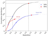 |
Fig. 1. Redshift cumulative distributions. Red, blue, and black lines correspond to the Pantheon, quasar, and SN-Q samples, respectively. The SNe Ia account for 42% of the SN-Q sample and the quasars for 58%. |
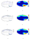 |
Fig. 2. Distributions and density contours in the galactic coordinate system. Panels a, c, and e: are the coordinate distributions of the Pantheon, quasar, and SN-Q samples in the galactic coordinate system, respectively. The corresponding density contours are described in panels b, d, and f. |
The cosmic anisotropy obtained from the SNe sample might rely on the inhomogeneous distribution of SNe Ia. The distributions of SNe Ia from the Pantheon sample are shown in panel a of Fig. 2. It is obvious that the belt part (the SDSS sample) plays a major role in the full Pantheon sample. To make it easier to comprehend this focus, we plotted the density distribution of the Pantheon sample, which is shown in panel b of Fig. 2. Zhao et al. (2019) analyzed the effect of the inhomogeneous distribution of the Pantheon sample on the cosmic anisotropy and found that the SDSS sample plays the most important role in the Pantheon sample. From panels c and d of Fig. 2, we find that the distribution of the quasar sample is more homogeneous and its maximum density value is smaller than that of the Pantheon sample. Compared with the Pantheon sample, adding the quasar sample reduces the unevenness of the overall sample and weakens the decisive role of the SDSS subsample as shown in panels e and f of Fig. 2. By combining Figs. 1 and 2, we find that the SN-Q sample is better than the Pantheon sample in terms of quantity, redshift range, and the uniform of distribution. However, the unevenness may not have been eliminated. It is obvious that the data number of the North Galactic Hemisphere is larger than the South Galactic Hemisphere in the quasar sample. Through statistics, the data number of the South and North Galactic Hemispheres in the Pantheon sample, quasar sample, and SN-Q sample are (644, 404), (438, 983), and (1082, 1387), respectively. The same case also appears in the SN-Q sample. In order to neutralize the inhomogeneous Pantheon sample, it might be necessary to obtain a larger and more homogeneous sample.
2.2. The MCMC method
For the standard cosmological model, the theoretical distance modulus can be written as
 (1)
(1)
where dL is the luminosity distance. In the flat ΛCDM model, dL can be calculated from
 (2)
(2)
where c is the speed of light, H0 is the Hubble constant, and Ωm is the matter density. For SNe Ia, the best fitting value of Ωm is achieved by minimizing the value of χ2
 (3)
(3)
where σi(zi) is the observational uncertainty of the distance modulus.
For quasars, the relation between UV and X-ray luminosities can be parameterized as (Avni & Tananbaum 1986)
 (4)
(4)
where LX is the rest-frame monochromatic luminosity at 2 keV and LUV is the luminosity at 2500 Å. We note that γ and β are two free parameters. Considering  , Eq. (4) can be written as
 (5)
(5)
From Eq. (5), we derive the theoretical X-ray flux (Khadka & Ratra 2020),
![Mathematical equation: $$ \begin{aligned} \phi ([F_{\rm UV}]_{i},d_{\rm L}[z_{i}])&=\log _{10}(F_{\rm X}) \nonumber \\&= \gamma (\log {F_{\rm UV}}) +(\gamma -1)\log {4\pi } \nonumber \\&\quad + 2(\gamma -1)\log _{10}{d_{\rm L}} + \beta . \end{aligned} $$](/articles/aa/full_html/2020/11/aa38541-20/aa38541-20-eq12.gif) (6)
(6)
For the quasar sample, the form of  related to the X-ray flux FX of the quasar is given as
![Mathematical equation: $$ \begin{aligned} \chi ^{2}_{\rm Q} =&\sum _{i=1}^{1421}\left(\frac{(\log _{10}(F_{\rm X})_{i}-\phi ([F_{\rm UV}]_{i},d_{\rm L}[z_{i}]))^{2}}{s_{i}^{2}} + \ln (2\pi s_{i}^{2})\right), \end{aligned} $$](/articles/aa/full_html/2020/11/aa38541-20/aa38541-20-eq14.gif) (7)
(7)
where the variance  consists of the global intrinsic δ and the measurement error σi in (FX)i, that is,
  . The function ϕ corresponds to the theoretical X-ray flux (Eq. (4)). Compared to δ and
  , the error of (FUV)i is negligible.
In substituting Eq. (6) for Eq. (7) and minimizing the value of  , we obtain the best-fit parameters: Ωm = 0.74
 , δ = 0.23
 , γ = 0.62
 , and β = 7.53
 . It is important to note that Ωm is in 4σ tension with the ΛCDM model (Risaliti & Lusso 2019). By combining Eqs. (1), (3), (6), and (7), the χ2 statistic for the SN-Q sample is
![Mathematical equation: $$ \begin{aligned} \chi ^{2}_{\rm Total}&= \chi ^{2}_{\rm SN} + \chi ^{2}_{\rm Q} \nonumber \\&=\sum _{i=1}^{1048}\frac{(\mu _{\rm obs}(z_{i}) - \mu _{\rm th}(\Omega _{\rm m},z_{i}))^{2}}{\sigma ^{2}} \nonumber \\&\quad +\sum _{i=1}^{1421}\left(\frac{(\log _{10}(F_{\rm X})_{i}-\phi ([F_{\rm UV}]_{i},d_{\rm L}[z_{i}]))^{2}}{s_{i}^{2}} + \ln (2\pi s_{i}^{2})\right). \end{aligned} $$](/articles/aa/full_html/2020/11/aa38541-20/aa38541-20-eq23.gif) (8)
(8)
By using Eq. (8), the best-fit parameters are Ωm = 0.29 , δ = 0.23
 , γ = 0.64
 , and β = 6.98
 from the SN-Q sample, which is shown in Fig. 3. The result is consistent with the ΛCDM model.
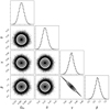 |
Fig. 3. Confidence contours (1σ, 2σ, and 3σ) and the marginalized likelihood distributions for the space of the parameters (Ωm, δ, γ, β) from the SN-Q sample in the spatially flat ΛCDM model. |
From the best-fit parameters for the quasar and SN-Q samples, we find that when only considering the quasar sample, the matter density Ωm = 0.74 . This is a significant departure from the Ωm given by the standard cosmological model. But Ωm = 0.29
 from the SN-Q sample is consistent with the standard cosmological model. This may imply that the quasars could not be used for the cosmological probe independently at present (Velten & Gomes 2020). It can be combined with others probes, for instance, SNe Ia, CMB, GRBs (Wang et al. 2015), and fast radio bursts (Yu & Wang 2017).
3. Testing the cosmic anisotropy with the HC and DF methods
3.1. The HC method and results
The HC method was first proposed by Schwarz & Weinhorst (2007); it is widely used to investigate the cosmic anisotropy. For example, the anisotropy of cosmic expansion, the temperature anisotropy of the CMB (Bennett et al. 2013; Eriksen et al. 2004; Planck Collaboration XXIII 2014; Akrami et al. 2014; Hansen et al. 2004; Quartin & Notari 2015), and the acceleration scale of modified Newtonian dynamics (Zhou et al. 2017; Chang et al. 2018b; Chang & Zhou 2019). Firstly, we briefly introduce this approach. Its goal is to identify the direction, which corresponds to the axis of maximal asymmetry from the dataset, by comparing the accelerating expansion rate. In the spatially flat ΛCDM model, it is convenient to employ Ωm to replace the accelerating expansion rate considering the relationship between the deceleration parameter q0 and Ωm. The most important step is to produce random directions  (l, b), which are used to split the dataset into two parts (defined as “up” and “down”), where l ∈ (0°, 360° ) and b ∈ ( − 90°, 90° ) are the longitude and latitude in the galactic coordinate system, respectively. According to “up” and “down” subdatasets, the corresponding best-fit values of Ωm, u and Ωm, d are obtained adopting the MCMC method. The nuisance parameters (δ, γ and β) are marginalized along with Ωm in the MCMC process. The anisotropy level (AL) made up of Ωm, u and Ωm, d can be used to describe the accelerating expansion rate.
In this section, we adopt the HC method and use the SN-Q sample to study the cosmic anisotropy. The AL is defined as
 (9)
(9)
where Ωm, u and Ωm, d are the best-fit Ωm of the “up” subset and “down” subset, respectively. These two subsets are distinguished from the full SN-Q sample by a random direction  . The 1σ uncertainty σAL is
 (10)
(10)
During the calculation, we repeated 3000 random directions  for the HC method and the results are
  = 0.407 and
  = 0.422, and the corresponding errors are
  = 0.0149 and
  = 0.0156. Then, we obtain the 1σ uncertainty σAL = 0.026. The anisotropic level with 1σ uncertainty is
 (11)
(11)
and the corresponding direction is
 (12)
(12)
The distribution of AL(l, b) is shown in Fig. 4. This preferred direction is inconsistent with the previous results with the Pantheon sample from the HC method. For instance, by employing the HC method, Deng & Wei (2018b) obtained two preferred directions (138.8°, −6.8°) and (102.36°, −28.58°) from the Pantheon sample. In using the same sample, Sun & Wang (2018) and Zhao et al. (2019) achieved the HC preferred direction (l, b) = (37°, 33°) and (l, b) = (123.05°, 4.78°), respectively. These four directions are plotted in Fig. 5. From the result of the HC method, it shows that the quasar sample has an obvious impact on the HC results.
 |
Fig. 4. Distribution of the AL in the galactic coordinate system. The triangle marks the direction of the largest of the AL in the sky. |
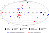 |
Fig. 5. Distribution of the preferred directions (l, b) in the various observational datasets. The blue color and red color correspond to the HC method and the DF method, respectively. |
We also assessed statistical significance of the results found by means of this test with simulated datasets. The simulated SN-Q datasets have the same direction in the sky as real data, but a different distance modulus (SNe Ia) and X-ray flux (quasar). Then the corresponding distance modulus and X-ray flux were constructed by the Gaussian function with the mean determined by Eq. (8), where Ωm = 0.29, δ = 0.23, γ = 0.64, β = 6.98 is the best-fitting value to the SN-Q sample and the standard deviation equal to the corresponding real datapoint 1σ error. Therefore, we constructed 200 simulated datasets and obtain the corresponding ALmax by employing the HC method. The distribution of ALmax in these datasets was fitted by a Gaussian function with the mean value 0.104 and the standard deviation 0.032, as shown in Fig. 6. From Fig. 6, we can find that the statistical significance of the maximum anisotropy level of ALmax, which is about 1.23σ and 14% of ALmax obtained from the simulated datasets, is greater than that of the real data. Therefore, the value of ALmax is not large enough. In addition, it is necessary to examine whether the maximum AL from the SN-Q sample is consistent with statistical isotropy. In order to determine this, we evenly redistributed the original data-sets across the sky and repeated it 200 times. The result of the simulated isotropic datasets is shown in Fig. 7. The mean value is 0.099 and the standard deviation is 0.024. We note that 7% of ALmax obtained from the simulated isotropic datasets is larger than that of the real data. The statistical significance of ALmax is about 1.65σ. The results of the random and isotropic datasets are smaller than 2σ, which still supports the absence of significant anisotropy.
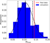 |
Fig. 6. Distribution of ALmax in 200 simulated datasets. The black curve is the best fitting result to the Gaussian function. The solid black and vertical dashed lines are commensurate with the mean and the standard deviation, respectively. The vertical red line shows the maximum AL derived from the actual SN-Q sample. |
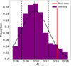 |
Fig. 7. Distribution of ALmax in 200 simulated isotropic datasets. The black curve is the best fitting result to the Gaussian function. The solid black and vertical dashed lines are commensurate with the mean and the standard deviation, respectively. The vertical red line shows the maximum AL derived from the actual SN-Q sample. |
In the end of this subsection, we compare the HC preferred direction of the SN-Q sample with those derived in various observational datasets. In Fig. 5, we plotted the preferred directions (l, b) found from various observational datasets by the HC method in the galactic coordinate system. From Fig. 5, we find that the HC preferred direction in this paper is the deviation from that of the Pantheon sample and the SPARC galaxies sample, but it is generally consistent with those in the Union2 sample (Antoniou & Perivolaropoulos 2010; Cai & Tuo 2012; Chang & Lin 2015), the Union2.1 sample (Sun & Wang 2019; Lin et al. 2016a), the Constitution sample (Sun & Wang 2019; Kalus et al. 2013), and the JLA sample (Deng & Wei 2018b). Overall, the distribution of the HC preferred direction obtained from a different sample is diffuse. As discussed by Sun & Wang (2019) and Zhao et al. (2019), the cosmic anisotropy found in the supernova sample significantly relies on the inhomogeneous distribution of SNe Ia in the sky. The preferred directions in various observational datasets are also shown in Table 1. From Table 1, we find that the HC preferred direction in this paper is also in agreement with the results of the CMB dipole (Lineweaver et al. 1996), velocity flows (Watkins et al. 2009; Feldman et al. 2010), quasar alignment (Hutsemékers et al. 2005; Hutsemékers 2011; Hutsemékers & Lamy 2001), the CMB quadrupole (Bielewicz et al. 2004; Frommert & Enßlin 2010), the CMB octopole (Bielewicz et al. 2004), △α/α (Webb et al. 2011; King et al. 2012), and infrared galaxies (Yoon et al. 2014; Bengaly et al. 2017).
Preferred directions (l, b) found in different cosmological models using different methods and observational datasets.
3.2. The DF method and results
The DF method is also used to test the cosmic anisotropy. Considering the dipole magnitude A and monopole term B, the theoretical distance modulus should be rewritten as
 (13)
(13)
where  and
and  correspond to the dipole direction and the unit vector pointing to the position of the SN Ia or quasar, respectively. In the galactic coordinate,
  is written as
 (14)
(14)
For any ith(li, bi) data points,  is given by
 (15)
(15)
We were able to obtain the best-fit dipole direction (l, b) by substituting Eq. (13) for Eq. (3) and minimizing χ2. Equation (13) can be directly used for the SNe Ia sample. For the quasars, according to Eq. (1), the theoretical distance modulus can also be written as
 (16)
(16)
In substituting Eq. (16) for Eq. (13), we obtain
 (17)
(17)
Thus the theoretical X-ray flux with dipole and monopole corrections is given by
![Mathematical equation: $$ \begin{aligned} \tilde{\phi }([F_{\rm UV}]_{i}, d_{\rm L}[z_{i}]) =&\gamma (\log {F_{\rm UV}}) +(\gamma -1)\log {4\pi } + \beta \nonumber \\& + 2(\gamma -1)\left(\log _{10} \frac{d_{\rm L}}{\mathrm{Mpc}} + 5\right) \nonumber \\& \times (1+A(\hat{\boldsymbol{n}}\cdot \hat{\boldsymbol{p}}) + B) - 5. \end{aligned} $$](/articles/aa/full_html/2020/11/aa38541-20/aa38541-20-eq102.gif) (18)
(18)
Adding Eqs. (13) and (18) to (8) and minimizing the value of  , the marginalized posterior distribution for the SN-Q sample is shown in Fig. 8. In total, there are eight parameters in the DF method, four of which are used to describe the universal anisotropy, that is, l, b, A, and B. The results show that the dipole direction (l, b) is (
 ,
,  ), the dipole magnitude A = (−4.36
 ) × 10−4 and the monopole term B = (−6.60
 ) × 10−5. The dipole direction is generally consistent with the preferred direction
  ,
,  of the HC method. Both the dipole magnitude A and monopole term B are approximately equal to zero, indicating that there is no significant anisotropy in the SN-Q sample. Next, we carry out a redshift tomography analysis to discuss the effect of redshift. The results of the redshift tomography analysis were calculated, as shown in Table 2. Based on analyses of Fig. 1, the number of low redshift sources is relatively large, so the redshift intervals are not uniform in the redshift tomography analysis. From the results of redshift tomography, it can be found that the dipole directions are distributed in a relatively small range. The maximum of monopole term A and the dipole magnitude B are near zero. There is no significant change in the dipole direction and anisotropic level with different redshift ranges. We note that |A| and |B| of the first bin are larger than that of others bins. This indicates that the anisotropy level of the low redshift range might be relatively higher.
 |
Fig. 8. Confidence contours (1σ, 2σ, and 3σ) and marginalized likelihood distributions for the parameters space (Ωm, δ, γ, β, l, b, A, B) to the SN-Q sample in the dipole-modulated ΛCDM model. |
Redshift tomography results using dipole fitting method for the SN-Q sample.
At the end of this section, we make a comparison between the dipole directions of the SN-Q sample with that derived from other samples and compare the results between the HC method and the DF method for the same sample. At first, we marked the dipole directions obtained from different samples in the galactic coordinate system, as shown in Fig. 5. The dipole directions obtained from different samples are mostly located in a relatively small part of the South Galactic Hemisphere. The dipole direction in this paper is inconsistent with them. The longitude l is close, but the deviation of latitude b is large. It might be caused by the inhomogeneous distribution of SNe Ia, as discussed in Sect. 2.1. The data number of the SN-Q sample in the North Galactic Hemisphere is larger than that in the South Galactic Hemisphere. But the dipole direction is in agreement with the results derived for the CMB dipole, velocity flows, quasar alignment, the CMB quadrupole, the CMB octopole, and △α/α. For the same sample, we find that the results of these two methods are not always consistent with each other. For instance, these two preferred directions obtained by the HC and DF methods in the SPARC galaxies sample (Zhou et al. 2017; Chang et al. 2018b), the Union2 sample (Antoniou & Perivolaropoulos 2010; Mariano & Perivolaropoulos 2012; Cai & Tuo 2012; Cai et al. 2013; Chang & Lin 2015), and the JLA sample (Bengaly et al. 2015; Sun & Wang 2019; Lin et al. 2016b; Deng & Wei 2018b), are consistent. However, the HC and DF preferred directions obtained from the Constitution sample (Sun & Wang 2019; Kalus et al. 2013) are inconsistent. The same case is also exhibited in the Pantheon sample (Sun & Wang 2018; Zhao et al. 2019; Deng & Wei 2018a). This may be due to the sensitivity of the two methods (Chang & Lin 2015).
In Table 1, we summarize the preferred directions (l, b) found in different cosmological models using different methods and observational datasets. The parts of the DF method and HC method have been discussed at the beginning of this section. In addition, we also summarize the research results obtained by various methods for different models (ΛCDM, wCDM, and CPL). Looking through the results from the same sample, we find that the results are almost independent of these three models.
4. Summary
The cosmic principle assumes that the universe is homogeneous and isotropic on cosmic scales. The research on cosmic anisotropy from SNe Ia also shows that there is no obvious anisotropy. In this work, we test the cosmic anisotropy with a new sample, which consists of SNe Ia and the quasars, by using the HC and DF methods. Nevertheless, the results show that there is no obvious anisotropy.
Firstly, we briefly investigate the Pantheon sample and quasar sample. By assessing the results, we find that adding the quasar sample reduces the unevenness of the overall sample. Compared with the Pantheon sample, the new sample (SN-Q sample) has a larger size, wider range of redshift, and a more uniform distribution. But the distribution of the SN-Q sample is still inhomogeneous in the North Galactic Hemisphere and South Galactic Hemisphere. We also briefly discuss the effect of inhomogeneous distribution on the dipole preferred in the SN-Q sample. By adopting the MCMC method, we obtain the best fitting values of Ωm, δ, γ, and β and find that 4σ tensions exist between the best-fit value of Ωm from the quasar sample and that of the ΛCDM model. Then, by adding the Pantheon sample into the quasar sample, the 4σ tension disappears.
For the HC method, the preferred direction that corresponds to the maximum accelerating expansion is  ,
,  . The anisotropy level ALmax is equal to 0.142 ± 0.026. By using the simulated datasets, we assess the HC result and determine that the statistical significance is about 1.23σ. In addition, we also examine whether the ALmax from the SN-Q sample is consistent with statistical isotropy by employing the simulated isotropic datasets. The statistical significance is about 1.65σ. The results show that it is hardly reproduced by simulated datasets or isotropy simulated datastes. For the DF method, we find that the preferred direction in the SN-Q sample points toward (
 ,
,  ) with an anisotropy level of A = (−4.36
 ) × 10−4, which is marginally consistent with the result of the HC method. There is a considerable deviation for the latitude direction l from those obtained from other SNe Ia samples, which may be caused by including the quasar sample. The preferred directions obtained by using the HC method and the DF method from the SN-Q sample are both in agreement with the results of the CMB dipole, velocity flows, quasar alignment, the CMB quadrupole, the CMB octopole, and △α/α. The results of the redshift tomographic analysis show that the dipole direction is weakly dependent on redshift. Comparing this with previous studies of the Pantheon sample, the preferred directions in the SN-Q sample have an obvious divergence. There does not exist an obvious anisotropy from the SN-Q sample.
Although the SN-Q sample is better than the Pantheon sample in some aspects, such as the quantity, redshift range, and uniform of distribution, there are still some shortcomings. For example, the distribution of the SN-Q sample is not uniform in the whole sky. Next-generation X-ray surveys, such as eROSITA, will provide us with larger and more precise luminosity distance determinations of quasars, so that we should be able to reduce the uncertainties obtained in our analysis. By employing a simulated e-ROSITA quasar sample, predictions for e-ROSITA from a quasar Hubble diagram have been made by Lusso (2020). Colin et al. (2019) point out that the cosmic acceleration is due to a non-negligible dipole anisotropy by analyzing the JLA sample. We think that the same research can be performed by a combined sample of SNe Ia and quasars, considering the quasar sample enables us to talk about this study in a higher redshift range and to test whether the same result will still be obtained. This will be pursued in future work.
Acknowledgments
We thank the anonymous referee for valuable comments. This work is supported by the National Natural Science Foundation of China (grant U1831207).
References
- Akrami, Y., Fantaye, Y., Shafieloo, A., et al. 2014, ApJ, 784, L42 [NASA ADS] [CrossRef] [Google Scholar]
- Alonso, A. I., Salvador, A. I., Sánchez, F. J., et al. 2015, MNRAS, 449, 670 [NASA ADS] [CrossRef] [Google Scholar]
- Amanullah, R., Lidman, C., Rubin, D., et al. 2010, ApJ, 716, 712 [NASA ADS] [CrossRef] [Google Scholar]
- Andrade, U., Bengaly, C. A. P., Alcaniz, J. S., & Santos, B. 2018, Phys. Rev. D, 97, 083518 [CrossRef] [Google Scholar]
- Antoniou, I., & Perivolaropoulos, L. 2010, JCAP, 2010, 012 [NASA ADS] [CrossRef] [Google Scholar]
- Avni, Y., & Tananbaum, H. 1986, ApJ, 305, 83 [NASA ADS] [CrossRef] [Google Scholar]
- Bengaly, C. A. P., Bernui, A., & Alcaniz, J. S. 2015, ApJ, 808, 39 [NASA ADS] [CrossRef] [Google Scholar]
- Bengaly, C. A. P., Alcaniz, J. S., Xavier, H. S., et al. 2017, MNRAS, 464, 768 [NASA ADS] [CrossRef] [Google Scholar]
- Bengaly, C. A. P., Novaes, C. P.,Xavier, H. S., et al. 2018a, MNRAS, 475, L106 [CrossRef] [Google Scholar]
- Bengaly, C. A. P., Maartens, R., & Santos, M. G. 2018b, JCAP, 04, 031 [Google Scholar]
- Bennett, C. L., Larson, D., Weiland, J. L., et al. 2013, ApJS, 208, A20 [Google Scholar]
- Betoule, M., Kessler, R., Guy, J., et al. 2014, A&A, 568, A22 [NASA ADS] [CrossRef] [EDP Sciences] [Google Scholar]
- Bielewicz, P., Górski, K. M., & Banday, A. J. 2004, MNRAS, 355, 1283 [NASA ADS] [CrossRef] [Google Scholar]
- Bisogni, S., Risaliti, G., & Lusso, E. 2017, Front. Astron. Space Sci., 4, 68 [NASA ADS] [CrossRef] [Google Scholar]
- Bonvin, C., Durrer, R., & Kunz, M. 2006, Phys. Rev. Lett., 96, 191302 [NASA ADS] [CrossRef] [Google Scholar]
- Brusa, M., Civano, F., Comastri, A., et al. 2010, ApJ, 716, 348 [NASA ADS] [CrossRef] [Google Scholar]
- Cai, R.-G., & Tuo, Z.-L. 2012, JCAP, 2012, 004 [NASA ADS] [CrossRef] [Google Scholar]
- Cai, R.-G., Ma, Y.-Z., Tang, B., & Tuo, Z.-L. 2013, Phys. Rev. D, 87, 123522 [CrossRef] [Google Scholar]
- Cai, R.-G., Liu, T.-B., Wang, S.-J., & Xu, W.-T. 2019, JCAP, 2019, 016 [CrossRef] [Google Scholar]
- Chang, Z., & Lin, H.-N. 2015, MNRAS, 446, 2952 [CrossRef] [Google Scholar]
- Chang, Z., & Zhou, Y. 2019, MNRAS, 486, 1658 [CrossRef] [Google Scholar]
- Chang, Z., Lin, H.-N., Sang, Y., & Wang, S. 2018a, MNRAS, 478, 3633 [CrossRef] [Google Scholar]
- Chang, Z., Lin, H.-N., Zhao, Z.-C., & Zhou, Y. 2018b, Chin. Phys. C, 42, 115103 [CrossRef] [Google Scholar]
- Clarkson, C., & Maartens, R. 2010, Class. Quant. Grav., 27, 124008 [NASA ADS] [CrossRef] [Google Scholar]
- Colin, J., Mohayaee, R., Sarkar, S., & Shafieloo, A. 2011, MNRAS, 414, 264 [NASA ADS] [CrossRef] [Google Scholar]
- Colin, J., Mohayaee, R., Rameez, M., & Sarkar, S. 2017, MNRAS, 471, 1045 [NASA ADS] [CrossRef] [Google Scholar]
- Colin, J., Mohayaee, R., Rameez, M., & Sarkar, S. 2019, A&A, 631, L13 [NASA ADS] [CrossRef] [EDP Sciences] [Google Scholar]
- Copi, C. J., Huterer, D., Schwarz, D. J., & Starkman, G. D. 2015, MNRAS, 449, 3458 [NASA ADS] [CrossRef] [Google Scholar]
- Deng, H.-K., & Wei, H. 2018a, Eur. Phys. J. C, 78, 755 [CrossRef] [EDP Sciences] [Google Scholar]
- Deng, H.-K., & Wei, H. 2018b, Phys. Rev. D, 97, 123515 [CrossRef] [Google Scholar]
- Eriksen, H. K., Hansen, F. K., Banday, A. J., et al. 2004, ApJ, 605, 14 [NASA ADS] [CrossRef] [Google Scholar]
- Feindt, U., Kerschhaggl, M., Kowalski, M., et al. 2013, A&A, 560, A90 [NASA ADS] [CrossRef] [EDP Sciences] [Google Scholar]
- Feldman, H. A., Watkins, R., & Hudson, M. J. 2010, MNRAS, 407, 2328 [NASA ADS] [CrossRef] [Google Scholar]
- Frommert, M., & Enßlin, T. A. 2010, MNRAS, 403, 1739 [NASA ADS] [CrossRef] [Google Scholar]
- Gibelyou, C., & Huterer, D. 2012, MNRAS, 427, 1994 [NASA ADS] [CrossRef] [Google Scholar]
- Górski, K. M., Hivon, E., Banday, A. J., et al. 2005, ApJ, 622, 759 [NASA ADS] [CrossRef] [Google Scholar]
- Gruppuso, A., Finelli, F., Natoli, P., et al. 2011, MNRAS, 411, 1445 [NASA ADS] [CrossRef] [Google Scholar]
- Hansen, F. K., Banday, A. J., & Górski, K. M. 2004, MNRAS, 354, 641 [NASA ADS] [CrossRef] [Google Scholar]
- Heneka, C., Marra, V., & Amendola, L. 2014, MNRAS, 439, 1855 [NASA ADS] [CrossRef] [Google Scholar]
- Hinshaw, G., Larson, D., Komatsu, E., et al. 2013, ApJS, 208, A19 [NASA ADS] [CrossRef] [Google Scholar]
- Hutsemékers, D., & Lamy, H. 2001, A&A, 367, 381 [NASA ADS] [CrossRef] [EDP Sciences] [Google Scholar]
- Hutsemékers, D., Cabanac, R., Lamy, H., & Sluse, D. 2005, A&A, 441, 915 [NASA ADS] [CrossRef] [EDP Sciences] [Google Scholar]
- Hutsemékers, D., Payez, A., Cabanac, R., et al. 2011, ASP Conf. Ser., 449, 441 [Google Scholar]
- Javanmardi, B., & Kroupa, P. 2017, A&A, 597, A120 [NASA ADS] [CrossRef] [EDP Sciences] [Google Scholar]
- Javanmardi, B., Porciani, C., Kroupa, P., & Pflamm-Altenburg, J. 2015, ApJ, 810, 47 [NASA ADS] [CrossRef] [Google Scholar]
- Kalfountzou, E., Civano, F., Elvis, M., et al. 2014, MNRAS, 445, 1430 [NASA ADS] [CrossRef] [Google Scholar]
- Kalus, B., Schwarz, D. J., Seikel, M., & Wiegand, A. 2013, A&A, 553, A56 [NASA ADS] [CrossRef] [EDP Sciences] [Google Scholar]
- Kazantzidis, L., & Perivolaropoulos, L. 2020, Phys. Rev. D, 102, 023520 [CrossRef] [Google Scholar]
- Khadka, N., & Ratra, B. 2020, MNRAS, 492, 4456 [CrossRef] [Google Scholar]
- Khodyachikh, M. F. 1989, Sov. Sci. Astron. Obs., 61, 101 [Google Scholar]
- Kim, J., & Naselsky, P. 2010, ApJ, 714, L265 [NASA ADS] [CrossRef] [Google Scholar]
- King, J. A., Webb, J. K., Murphy, M. T., et al. 2012, MNRAS, 422, 3370 [NASA ADS] [CrossRef] [Google Scholar]
- Koivisto, T., & Mota, D. F. 2008, JCAP, 2008, 018 [NASA ADS] [CrossRef] [Google Scholar]
- Li, X., Lin, H.-N., Wang, S., & Chang, Z. 2013, Eur. Phys. J. C, 73, 2653 [CrossRef] [EDP Sciences] [Google Scholar]
- Lin, H.-N., Li, X., & Chang, Z. 2016a, MNRAS, 460, 617 [NASA ADS] [CrossRef] [Google Scholar]
- Lin, H.-N., Wang, S., Chang, Z., & Li, X. 2016b, MNRAS, 456, 1881 [NASA ADS] [CrossRef] [Google Scholar]
- Lineweaver, C. H., Tenorio, L., Smoot, G. F., et al. 1996, ApJ, 470, 38 [NASA ADS] [CrossRef] [Google Scholar]
- Lusso, E. 2020, Front. Astron. Space Sci., 7, 8 [CrossRef] [Google Scholar]
- Lusso, E., & Risaliti, G. 2016, ApJ, 819, 154 [NASA ADS] [CrossRef] [Google Scholar]
- Lusso, E., & Risaliti, G. 2017, A&A, 602, A79 [NASA ADS] [CrossRef] [EDP Sciences] [Google Scholar]
- Lusso, E., Comastri, A., Vignali, C., et al. 2010, A&A, 512, A34 [NASA ADS] [CrossRef] [EDP Sciences] [Google Scholar]
- Lusso, E., Piedipalumbo, E., Risaliti, G., et al. 2019, A&A, 628, L4 [NASA ADS] [CrossRef] [EDP Sciences] [Google Scholar]
- Mariano, A., & Perivolaropoulos, L. 2012, Phys. Rev. D, 86, 083517 [NASA ADS] [CrossRef] [Google Scholar]
- Melia, F. 2019, MNRAS, 489, 517 [CrossRef] [Google Scholar]
- Migkas, K., Schellenberger, G., Reiprich, T. H., et al. 2020, A&A, 636, A15 [CrossRef] [EDP Sciences] [Google Scholar]
- Pâris, I., Petitjean, P., Ross, N. P., et al. 2017, A&A, 597, A79 [NASA ADS] [CrossRef] [EDP Sciences] [Google Scholar]
- Pelgrims, V., & Hutsemékers, D. 2016, A&A, 590, A53 [NASA ADS] [CrossRef] [EDP Sciences] [Google Scholar]
- Perivolaropoulos, L. 2014, Galaxies, 2, 22 [NASA ADS] [CrossRef] [Google Scholar]
- Planck Collaboration XXIII. 2014, A&A, 571, A23 [NASA ADS] [CrossRef] [EDP Sciences] [MathSciNet] [PubMed] [Google Scholar]
- Planck Collaboration XXVI. 2014, A&A, 571, A26 [CrossRef] [EDP Sciences] [Google Scholar]
- Planck Collaboration VII. 2020, A&A, 641, A7 [CrossRef] [EDP Sciences] [Google Scholar]
- Qiang, D. C., Deng, H. K., & Wei, H. 2019, Class. Quant. Grav., 37, 185022 [CrossRef] [Google Scholar]
- Qin, Y. P., Xie, G. Z., Wang, J. C., et al. 1997, Ap&SS, 253, 19 [CrossRef] [Google Scholar]
- Quartin, M., & Notari, A. 2015, JCAP, 2015, 008 [NASA ADS] [CrossRef] [Google Scholar]
- Reid, B. A., Percival, W. J., Eisenstein, D. J., et al. 2010, MNRAS, 404, 60 [NASA ADS] [CrossRef] [Google Scholar]
- Risaliti, G., & Lusso, E. 2015, ApJ, 815, 33 [NASA ADS] [CrossRef] [Google Scholar]
- Risaliti, G., & Lusso, E. 2019, Nat. Astron., 3, 272 [NASA ADS] [CrossRef] [Google Scholar]
- Rubart, M., & Schwarz, D. J. 2013, A&A, 555, A117 [NASA ADS] [CrossRef] [EDP Sciences] [Google Scholar]
- Salvestrini, F., Risaliti, G., Bisogni, S., et al. 2019, A&A, 631, A120 [CrossRef] [EDP Sciences] [Google Scholar]
- Schwarz, D. J., & Weinhorst, B. 2007, A&A, 474, 717 [NASA ADS] [CrossRef] [EDP Sciences] [Google Scholar]
- Scolnic, D. M., Jones, D. O., Rest, A., et al. 2018, ApJ, 859, 101 [NASA ADS] [CrossRef] [Google Scholar]
- Shen, Y., Richards, G. T., Strauss, M. A., et al. 2011, ApJS, 194, A45 [NASA ADS] [CrossRef] [Google Scholar]
- Singal, A. K. 2011, ApJ, 742, L23 [NASA ADS] [CrossRef] [Google Scholar]
- Singal, A. K. 2019, Phys. Rev. D, 100, 063501 [CrossRef] [Google Scholar]
- Sun, Z. Q., & Wang, F. Y. 2018, MNRAS, 478, 5153 [NASA ADS] [CrossRef] [Google Scholar]
- Sun, Z. Q., & Wang, F. Y. 2019, Eur. Phys. J. C, 79, 783 [CrossRef] [EDP Sciences] [Google Scholar]
- Suzuki, N., Rubin, D., Lidman, C., et al. 2012, ApJ, 746, 85 [NASA ADS] [CrossRef] [Google Scholar]
- Tegmark, M., de Oliveira-Costa, A., & Hamilton, A. J. 2003, Phys. Rev. D, 68, 123523 [NASA ADS] [CrossRef] [Google Scholar]
- Tiwari, P., & Nusser, A. 2016, JCAP, 03, 062 [Google Scholar]
- Tiwari, P., & Jain, P. 2019, A&A, 622, A113 [NASA ADS] [CrossRef] [EDP Sciences] [Google Scholar]
- Trujillo-Gomez, S., Klypin, A., Primack, J., & Romanowsky, A. J. 2011, ApJ, 742, 16 [NASA ADS] [CrossRef] [Google Scholar]
- Vagnetti, F., Antonucci, M., & Trevese, D. 2013, A&A, 550, A71 [NASA ADS] [CrossRef] [EDP Sciences] [Google Scholar]
- Velten, H., & Gomes, S. 2020, Phys. Rev. D, 101, 043502 [CrossRef] [Google Scholar]
- Wang, J. S., & Wang, F. Y. 2014, MNRAS, 443, 1680 [NASA ADS] [CrossRef] [Google Scholar]
- Wang, Y.-Y., & Wang, F. Y. 2018, MNRAS, 474, 3516 [CrossRef] [Google Scholar]
- Wang, F.-Y., Dai, Z. G., & Liang, E. W. 2015, New Astron. Rev., 67, 1 [NASA ADS] [CrossRef] [Google Scholar]
- Watkins, R., Feldman, H. A., & Hudson, M. J. 2009, MNRAS, 392, 743 [NASA ADS] [CrossRef] [Google Scholar]
- Webb, J. K., King, J. A., Murphy, M. T., et al. 2011, Phys. Rev. Lett., 107, 191101 [NASA ADS] [CrossRef] [Google Scholar]
- Wei, J.-J., & Melia, F. 2020, ApJ, 888, 99 [CrossRef] [Google Scholar]
- Weinberg, S. 1972, Gravitation and Cosmology (New York: Wiley) [Google Scholar]
- Weinberg, S. 2008, Cosmology (Oxford: Oxford University Press) [Google Scholar]
- Yang, X., Wang, F. Y., & Chu, Z. 2014, MNRAS, 437, 1840 [NASA ADS] [CrossRef] [Google Scholar]
- Yoon, M., Huterer, D., Gibelyou, C., et al. 2014, MNRAS, 445, L60 [NASA ADS] [CrossRef] [Google Scholar]
- Yu, H., & Wang, F. Y. 2017, A&A, 606, A3 [NASA ADS] [CrossRef] [EDP Sciences] [Google Scholar]
- Zhao, W. 2014, Phys. Rev. D, 89, 023010 [NASA ADS] [CrossRef] [Google Scholar]
- Zhao, W., Wu, P., & Zhang, Y. 2013, Int. J. Mod. Phys. D, 22, 1350060 [CrossRef] [Google Scholar]
- Zhao, D., Zhou, Y., & Chang, Z. 2019, MNRAS, 486, 5679 [CrossRef] [Google Scholar]
- Zhou, Y., Zhao, Z.-C., & Chang, Z. 2017, ApJ, 847, 86 [CrossRef] [Google Scholar]
All Tables
Preferred directions (l, b) found in different cosmological models using different methods and observational datasets.
All Figures
|
Fig. 1. Redshift cumulative distributions. Red, blue, and black lines correspond to the Pantheon, quasar, and SN-Q samples, respectively. The SNe Ia account for 42% of the SN-Q sample and the quasars for 58%. |
| In the text | |
|
Fig. 2. Distributions and density contours in the galactic coordinate system. Panels a, c, and e: are the coordinate distributions of the Pantheon, quasar, and SN-Q samples in the galactic coordinate system, respectively. The corresponding density contours are described in panels b, d, and f. |
| In the text | |
|
Fig. 3. Confidence contours (1σ, 2σ, and 3σ) and the marginalized likelihood distributions for the space of the parameters (Ωm, δ, γ, β) from the SN-Q sample in the spatially flat ΛCDM model. |
| In the text | |
|
Fig. 4. Distribution of the AL in the galactic coordinate system. The triangle marks the direction of the largest of the AL in the sky. |
| In the text | |
|
Fig. 5. Distribution of the preferred directions (l, b) in the various observational datasets. The blue color and red color correspond to the HC method and the DF method, respectively. |
| In the text | |
|
Fig. 6. Distribution of ALmax in 200 simulated datasets. The black curve is the best fitting result to the Gaussian function. The solid black and vertical dashed lines are commensurate with the mean and the standard deviation, respectively. The vertical red line shows the maximum AL derived from the actual SN-Q sample. |
| In the text | |
|
Fig. 7. Distribution of ALmax in 200 simulated isotropic datasets. The black curve is the best fitting result to the Gaussian function. The solid black and vertical dashed lines are commensurate with the mean and the standard deviation, respectively. The vertical red line shows the maximum AL derived from the actual SN-Q sample. |
| In the text | |
|
Fig. 8. Confidence contours (1σ, 2σ, and 3σ) and marginalized likelihood distributions for the parameters space (Ωm, δ, γ, β, l, b, A, B) to the SN-Q sample in the dipole-modulated ΛCDM model. |
| In the text | |
Current usage metrics show cumulative count of Article Views (full-text article views including HTML views, PDF and ePub downloads, according to the available data) and Abstracts Views on Vision4Press platform.
Data correspond to usage on the plateform after 2015. The current usage metrics is available 48-96 hours after online publication and is updated daily on week days.
Initial download of the metrics may take a while.