| Issue |
A&A
Volume 643, November 2020
|
|
|---|---|---|
| Article Number | A61 | |
| Number of page(s) | 32 | |
| Section | Interstellar and circumstellar matter | |
| DOI | https://doi.org/10.1051/0004-6361/202038457 | |
| Published online | 03 November 2020 | |
Mapping the H2D+ and N2H+ emission toward prestellar cores. Testing dynamical models of the collapse using gas tracers★
1
School of Physics & Astronomy, University of Leeds,
Woodhouse Lane,
LS2 9JT
Leeds, UK
e-mail: This email address is being protected from spambots. You need JavaScript enabled to view it.
2
IRAP, Université de Toulouse, CNRS, UPS, CNES,
31400
Toulouse, France
3
INAF-Osservatorio Astrofisico di Arcetri,
Largo E. Fermi 5,
50125
Florence, Italy
4
Herzberg Astronomy and Astrophysics Research Centre, National Research Council of Canada,
Victoria,
BC, Canada
5
SRON Netherlands Institute for Space Research,
Landleven 12,
9747 AD
Groningen, The Netherlands
6
Kapteyn Astronomical Institute, University of Groningen,
Groningen, The Netherlands
Received:
20
May
2020
Accepted:
18
September
2020
Abstract
Context. The study of prestellar cores is critical as they set the initial conditions in star formation and determine the final mass of the stellar object. To date, several hypotheses have described their gravitational collapse. Deriving the dynamical model that fits both the observed dust and the gas emission from such cores is therefore of great importance.
Aims. We perform detailed line analysis and modeling of H2D+ 110–111 and N2H+ 4–3 emission at 372 GHz, using 2′ × 2′ maps (James Clerk Maxwell Telescope; JCMT). Our goal is to test the most prominent dynamical models by comparing the modeled gas kinematics and spatial distribution (H2D+ and N2H+) with observations toward four prestellar (L1544, L183, L694-2, L1517B) and one protostellar core (L1521f).
Methods. We fit the line profiles at all offsets showing emission using single Gaussian distributions. We investigate how the line parameters (VLSR, FWHM and TA*) change with offset to examine the velocity field, the degree of nonthermal contributions to the line broadening, and the distribution of the material in these cores. To assess the thermal broadening, we derive the average gas kinetic temperature toward all cores using the non-LTE radiative transfer code RADEX. We perform a more detailed non-LTE radiative transfer modeling using RATRAN, where we compare the predicted spatial distribution and line profiles of H2D+ and N2H+ with observations toward all cores. To do so, we adopt the physical structure for each core predicted by three different dynamical models taken from literature: quasi-equilibrium Bonnor–Ebert sphere (QE-BES), singular isothermal sphere (SIS), and Larson–Penston (LP) flow. In addition, we compare these results to those of a static sphere, whose density and temperature profiles are based on the observed dust continuum. Lastly, we constrain the abundance profiles of H2D+ and N2H+ toward each core.
Results. We find that variable nonthermal contributions (variations by a factor of 2.5) are required to explain the observed line width of both H2D+ and N2H+, while the nonthermal contributions are found to be 50% higher for N2H+. The RADEX modeling results in average core column densities of ~9 × 1012 cm−2 for H2D+ and N2H+. The LP flow seems to be the dynamical model that can reproduce the observed spatial distribution and line profiles of H2D+ on a global scale of prestellar cores, while the SIS model systematically and significantly overestimates the width of the line profiles and underestimates the line peak intensity. We find similar abundance profiles for the prestellar cores and the protostellar core. The typical abundances of H2D+ vary between 10−9 and 10−10 for the inner 5000 au and drop by about an order of magnitude for the outer regions of the core (2 × 10⁻¹⁰–6 × 10⁻¹¹). In addition, a higher N2H+ abundance by about a factor of 4 compared to H2D+ is found toward the two cores with detected emission. The presence of N2H+ 4–3 toward the protostellar core and toward one of the prestellar cores reflects the increasing densities as the core evolves.
Conclusions. Our analysis provides an updated picture of the physical structure of prestellar cores. Although the dynamical models account for mass differences by up to a factor of 7, the velocity structure drives the shape of the line profiles, allowing for a robust comparison between the models. We find that the SIS model can be clearly excluded in explaining the gas emission toward the cores, but a larger sample is required to differentiate clearly between the LP flow, the QE-BES, and the static models. All models of collapse underestimate the intensity of the gas emission by up to several factors toward the only protostellar core in our sample, indicating that different dynamics take place in different evolutionary core stages. If the LP model is confirmed toward a larger sample of prestellar cores, it would indicate that they may form by compression or accretion of gas from larger scales. If the QE-BES model is confirmed, it means that quasi-hydrostatic cores can exist within turbulent ISM.
Key words: stars: formation / ISM: clouds / ISM: kinematics and dynamics / submillimeter: ISM
The reduced H2D+ and N2H+ JCMT data cubes of all cores are only available at the CDS via anonymous ftp to cdsarc.u-strasbg.fr (130.79.128.5) or via http://cdsarc.u-strasbg.fr/viz-bin/cat/J/A+A/643/A61
© ESO 2020
1 Introduction
Star formation begins within molecular clouds, where magnetic fields and turbulence dominate the dynamics, leading to the formation of filamentary structures of gas (Arzoumanian et al. 2011; Pudritz & Kevlahan 2013; André 2017). In particular, Herschel observations have revealed that prestellar cores and protostellar objects form in thermally critical and supercritical filaments (André et al. 2010; Tafalla & Hacar 2015). Understanding the physical and chemical processes that take place in these very early stages of star formation is of high importance. Not only do such cores set the initial conditions of star formation and determine the final mass of the star (Bergin & Tafalla 2007), but they also have a strong influence on the multiplicity (Pineda et al. 2015). Although low-mass star formation is better understood than high-mass star formation, the initial conditions of the collapse remain uncertain. Prestellar cores are known to contract under gravitational forces (Krumholz et al. 2005), while thermal and magnetic pressure and the presence of turbulence prevent the core from collapsing (Goodman et al. 1998).
The most broadly known dynamical models of a spherically symmetric collapsing core are: i) the Larson–Penston flow (LP flow; Larson 1969; Penston 1969), where at t ~0 the inflow velocity at large radii reaches supersonic values (~3.3 × speed of sound), and therefore is far from equilibrium, and the density profile follows a power-law; ii) the singular isothermal sphere (SIS) evolving via an “inside-out” collapse (Shu 1977); and iii) the hydrostatic Bonnor–Ebert sphere (BES) supported by turbulence, which, when disturbed, can lead to a contraction in quasi-equilibrium (QE; Broderick & Keto 2010). Constraining the dynamical structure of prestellar cores observationally is very challenging. Hence, detailed studies focusing on the gas emission, as well as the age determination of observed prestellar cores, are crucial to distinguish between the proposed models.
Ward-Thompson et al. (1994) presented the first submillimeter continuum survey of a sample of cores without associated infrared emission shortward of 100 μm, therefore presumably starless cores, reporting their first detection using longer wavelengths (>450 μm). The lifetime of prestellar cores has been observationally estimated to be ~ 104–106 yr (e.g., L1544, L694-2, L183 Beichman et al. 1986; Caselli et al. 2008; Enoch et al. 2008). The prestellar cores are characterized by very low temperatures (T ≈ 10 K) that increase outward, and high densities (>105 cm−3; Keto & Caselli 2008) that show a flattened density profile in the center, resulting in the unique gas chemistry presented in the current paper. Various studies have shown a strong correlation between CO depletion and the degree of deuteration of hydrogen-based species in prestellar cores (Caselli et al. 2003; Vastel et al. 2006). Below the critical temperature of T ≈ 25 K, gas-phase species, including almost all CNO species, are frozen out (≳98% Caselli et al. 2003)to dust grains and therefore are depleted (Caselli et al. 2008). The enrichment in H2D+ and N2H+ under those conditions can be understood if one takes a closer look at the production and destruction mechanisms of the relevant species (Eq. (1) to (4)):
 (1)
(1)
 (2)
(2)
 (3)
(3)
 (4)
(4)
As soon as CO returns to the gas-phase (T > 20–30 K, i.e., after the formation of a protostar), the abundance of both H2D+ and N2H+ will subsequently decrease. We note, however, that N2H+ survives with an abundance independent of the distance from the center (Pagani et al. 2012; Lique et al. 2015) and appears to remain longer (Tafalla et al. 2006).
Given the scarcity of available molecular tracers originating from prestellar cores, previous studies have naturally focused on H2D+ (Caselli et al. 2002, 2008; van der Tak et al. 2005; Vastel et al. 2006; Harju et al. 2006) and N2H+ (Tafalla et al. 2004; Pagani et al. 2007; Lique et al. 2015), using high resolution ground-based submm observatories (14′′ –22′′; JCMT, CSO). Those studies provided important constraints on the temperature structure of such cores and the column densities and abundances of molecular species at individual cores. Since then, the collisional data for both H2D+ (Hugo et al. 2009) and N2H+ (Lique et al. 2015) have been revised and therefore the reported properties of those clouds also need to be revised.
In the past decade, there have been several attempts to trace substructure via the dust continuum and molecular line emission within the central 1000 au of prestellar cores using interferometers, but mostly without positive results. There have been no fruitful detections of dust continuum at mm wavelengths toward single objects or toward a sample of cores in Perseus or Ophiuchusin the past (CARMA, IRAM, SMA; Schnee et al. 2012, 2010; Crapsi et al. 2007), explained by the shallow density profiles of prestellar cores at less than few thousand astronomical units. Due to the spatial capabilities and high sensitivity of the Atacama Large Millimeter and submillimeter Array (ALMA), a few studies have been able to detect some compact emission but without resolving the substructure (Friesen et al. 2014, 2018; Kirk et al. 2017). Only very recently have the inner regions of a single prestellar core been resolved for the first time (L1544 with ALMA; Caselli et al. 2019). Given the very challenging nature of the continuum observations at those high angular resolutions (50–100 au), it is no surprise that H2D+ detection with ALMA is limited to a single low-mass prestellar core (SM1N; Friesen et al. 2014). Therefore, the analysis and modeling of single-dish observations of dust and gas toward prestellar cores is still a powerful approach to probe these enigmatic stages of star formation.
In this paper, we present the first dedicated study to test the proposed dynamical models using advanced non-LTE radiative transfer modeling to simulate the gas emission, making use of the optically thin H2D+ 110 –111 and N2H+ 4–3 line emission mapped with the James Clerk Maxwell Telescope (JCMT) toward a sample of prestellar cores (4) and one protostellar core. In Sect. 2, we describe the target selection, observations and data reduction. In Sect. 3, we present the observed spatial distributions and line analyses of H2D+ and N2H+ toward all cores and we also investigated the thermal and nonthermal contributions to the observed line width. In Sect. 4, we present the average column densities of H2D+ and N2H+ as determined using a non-LTE radiative transfer code to fit the line emission at the central submm peak position toward all cores. In Sect. 5, we used a detailed radiative transfer model to simulate the 2′ × 2′ maps of the H2D+ and N2H+ line emission toward the cores, adopting three different dynamical models: quasi-equilibrium Bonnor–Ebert sphere (QE-BES), singular isothermal sphere (SIS), and Larston–Penston (LP) flow, and a static sphere. Our main results and conclusions are presented in Sect. 7.
2 Observations
2.1 Targets
In this study, we present the analysis of five cores. Their coordinates, distances and continuum brightnesses at 850 μm and the core masses (4–10 M⊙) based on dust and gasmm observations are presented in Table 1. These cores have been previously observed by Crapsi et al. (2005) in lines of N2H+ and N2D+ to explore the use of deuterium enrichment to constrain the evolutionary status of starless cores. The five cores of the present sample werespecifically selected from the 31 cores presented in Crapsi et al. (2005) to provide a sample whereby detection of H2D+ could be considered favorable, typically by a high ratio of N(N2D+/N2H+) (see Table 7; Crapsi et al. 2005). The present sample consists of four cores that are considered to be more evolved based on a variety of chemical and kinematical probes (L1544, L1521f, L694-2, L183) and one less evolved core (L1517B).
Of the five cores in Table 1, four contain no known young stellar objects and, therefore, can be considered starless. Only toward one core, L1521f, a very low luminosity object (VELLO) was identified by Bourke et al. (2006), and therefore it is considered to be protostellar (see also, Tokuda et al. 2016, 2017).
Source sample: positions, continuum brightness, and distance.
2.2 Submillimeter single-dish observations
The five cores in this study were observed from January 2007 to January 2008 as part of three semesters of queue-mode observing at the JCMT1 on Mauna Kea, Hawaii, under observing programs M06BC11, M07AC15, and M07BC06. All observations were made under very dry weather conditions (i.e., τ225 < 0.05), to ensure maximum sensitivity to the ortho-H2D+ 110 –111 line and the N2H+ 4–3 line (at 372.42 and 372.67 GHz, respectively; Pickett et al. 1998), which are adjacent to a broad atmospheric H2O feature. JCMT has a beamwidth of 14′′ at the relevant frequency band (350 GHz).
The observations were made using the 16-element Heterodyne Array Receiver Programme (HARP) focal-plane array that operates over 325–375 GHz and the AutoCorrelation Spectrometer Imaging System (ACSIS) back-end (Buckle et al. 2009). HARP was tuned to 372.5 GHz, and ACSIS configured to provide nominally 500 MHz total bandwidth with 61 kHz wide channels or 0.048 km s−1 spacing. This setup allowed both the H2D+ 110 –111 and N2H+ 4–3 lines to be observed simultaneously in the same spectral window. The velocity resolution of ACSIS data is a factor of ~1.2 less than the configured channel spacing, or in this case, 0.058 km s−1.
The observations were defined in minimum schedulable blocks (MSBs) and were preceded by standard focus calibration observations at 345 GHz on nearby bright objects like R Aql. Additionally, pointing calibrations at 345 GHz were conducted on objects such as CRL618, both before the program MSBs and every ~60–90 min. Flux calibration was monitored by observing when possible spectral line standards, like W75N, at a variety of frequencies. The aperture efficiency, ηα, of HARP at 372.5 GHz is ~0.5.
HARP consists of 16 receptors arranged in a 4 × 4 square pattern with an on-sky spacing between receptors of 30′′. Program MSBs were executed by pointing one of the inner four HARP receptors at the target positions of the cores (Table 1). Data were obtained by pointing HARP at the target positions, and integrating using a “stare-mode” fashion, through chopping between the target positions and positions 180′′ distant in azimuth at 7.8125 Hz. Each MSB consisted of five repeats of 300 s. Each target was observed for ~4 h in total. When H2D+ 110 –111 was detected at the target position by at levels ≥ ~5σ, the telescope was shifted diagonally in position by ~22.5′′, namely, the target position was centered in the array between the center four receptors, and further staring observations were to be executed for up to another ~4 h. This strategy allowed the acquisition of high sensitivity data of faint lines in a “checkerboard” pattern across each core at a spatial sampling better than given by a single HARP footprint. Observing each core with HARP in a jiggle pattern would have resulted in better spatial sampling but at the cost of sensitivity in each source. Since HARP is aligned on the JCMT in azimuth and elevation, the final data per pointing sometimes include samples of more than 16 positions on the sky due to field rotation. Additionally, the total integration duration varies from core to core, given the nature of queue-mode observing and the scarcity of very dry weather conditions.
2.3 Data reduction
The data were reduced using standard routines and procedures in the STARLINK reduction package2 (Currie et al. 2014). Each integration was visually checked for baseline ripples, absent detectors, or large spikes, and specific integrations where these occurred were removed from the data ensemble. In particular, receptor H03 was unavailable during most of the observations; at various times, no more than two other receptors were also unavailable. Less strong spikes were identified and removed using a standard methodology created by developers at the Joint Astronomy Centre. Spectral baselines were subtracted, frequency axes converted to velocities and spectra trimmed using STARLINK scripts. To increase the signal-to-noise ratio (S/N), we re-binned the velocity axes of all the data by applying a factor of 2, resulting in a spectral resolution of ~0.12 km s−1.
3 Observational results
3.1 Spatial distribution of H2D+ and N2H+
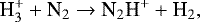
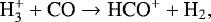
The observed spatial distributions of H2D+ 110 –111 emission toward all cores are presented in Fig. 1. H2D+ in emission is clearly seen toward each core of the sample. In all cases, the peak line brightness is found at the position of the 850 μm peak continuum emission (i.e., within a ~ 14′′ beam width). The line in emission is also clearly detected at several positions offset from the central position toward all cores. The observations of N2H+ 4–3 from the cores where it was clearly detected (L1521f and L1544) are presented in Fig. 2. The detection of this emission is spatially limited to two peaks toward L1521f and possibly L1544, and in particular, the second peak is at a location ~ 15′′ offset from the local peak of the submillimeter continuum emission.
 |
Fig. 1 Spatial distribution of H2D+ line emission as observed with JCMT toward the cores L1521f, L183, L1517B, L694-2, and L1544. The red cross indicates the peak of the 850 μm emission. The area filled with light green indicates the clear (>3σ) detections and the possible detections (~2σ) based on the line shape and peak velocity position. |
 |
Fig. 2 Spatial distribution of N2H+ 4–3 as observed with JCMT toward L1544 and L1521f. These two are the only cores with N2H+ 4–3 line emission detections. The area filled with light green indicates the clear (>3σ) detections and the possible detections (~2σ) based on the line shape and peak velocity position. |
3.2 Line profiles
We fit single Gaussians to the H2D+ 110 –111 and N2H+ 4–33 lines observed for each core and at each position where the emission is detected ( rms). Table 2 lists the peak brightness (
 ), central line velocity (VLSR), and the line width (FWHM) with the associated positions expressed in offsets from the local peak of the submillimeter 850 μm continuum emission.
Figures 3–7 show the derived line properties, VLSR, FHWM, and  of H2D+ and N2H+ emission with respect to their offsets from the 850 μm dust peak. Firstly, we plot the VLSR versus offsets and compare these to the known source velocities taken from the literature (e.g., Caselli et al. 2008). The upper plots in Figs. 3–7 show that the measured VLSR at the central position is in very good agreement and mostly within the errors when compared to the values reported by Caselli et al. (2008) toward most of the cores. Caselli et al. (2008) observed H2D+ with CSO and got measurements of the emission at the central position of those cores at a similar spectral resolution to the current study but a lower angular resolution (22′′ compared to our 14′′). In contrast, the source core velocity of L1544 reported by Ho et al. (1978) using NH3 measurements is systematically lower than those measured in our study and in Caselli et al. (2008) for the central positions. Instead, the measured velocities reported in Ho et al. (1978) come to a better agreement with those we find at offsets further out in the cloud. We should note that the angular resolution in the 1978 study was larger by a factor of >4. Taking all the above into consideration, we conclude that our measurements are consistent with previous work.
The FWHMs of the lines are of interest since they can provide information on whether the broadening of the emission is a result of only a thermal contribution or if nonthermal motions are also present at those very early stages of star formation. The line profiles of all five cores are characterized by narrow emission (0.2–0.6 km s−1). The thermal broadening (ΔVTHERM) is estimated using:
 (5)
(5)
where T is the gas kinetic temperature we determine for each individual core (6–9 K; see RADEX analysis in Sect. 4, Table 3), and m is the mass of the ion.
ΔVTHERM was thus found to be within 0.26–0.32 km s−1 for H2D+ and 0.09–0.11 km s−1 for N2H+. By determining the ΔVTHERM and measuring the observed line width of the species at each position in the maps, we can quantify how much of the observed line broadening is due to nonthermal contributions ( ; Myers et al. 1991) for each source (i.e., turbulence and magnetic fields). To address the significance of nonthermal contributions, we approached the temperature errors such that the temperature is within the range 5–12 K (typical values for dense cores).
Here, we present our findings regarding the entire sample, while more details on each individual core can be found in Appendix A. The middle plots in Figs. 3–7 show that thermal broadening alone is insufficient to explain the observed line widths toward most of the offset positions toward all cores. In particular, there is an indication that the nonthermal contributions become less significant for both H2D+ and N2H+ as one moves outward from the central position for three out of five cores. This finding contradicts the theory and what was previously observed toward molecular clouds, where the velocity dispersion increases with scale as the density decreases (e.g., Maloney 1988).
For the two cores for which both H2D+ and N2H+ measurements are available, we compared the nonthermal contribution at the central position. In particular, we find nonthermal contributions for H2D+ to be  km s−1 and
  km s−1 for L1544 and L1521f, respectively, while for N2H+ we find these to be
  km s−1 and 0.6 ± 0.1 km s−1, respectively.For L1544, the regions traced by the two species are characterized by similar nonthermal contributions (within the uncertainties) and, therefore, originate from regions with similar internal motions. For the more evolved, L1521f core, the nonthermal contributions are higher by a factor of 3 for the N2H+ line compared to the H2D+, which is beyond the uncertainties. This latter difference indicates that even though both lines are observed at a central position of the protostellar core, the H2D+ emission originates from more quiescent gas than the N2H+ emission does. This difference can be explained by the more complex structure of protostellar cores (i.e., outflow, disk) compared with prestellar cores.
Lastly, the  at each offset can provide valuable information regarding the gas density and temperature properties toward the cores. The lower plots in Figs. 3–7 suggest that
  generally decreases with increasing offset. This behavior can be explained by the decreasing density or decreasing excitation temperature, Tex (i.e., sub-thermal excitation), as one moves outward from the center of the core, and it is suggestive of the low optical depth of the line (see also Sect. 5.3). We note that the kinetic temperature in prestellar cores generally increases outward (up to 5 K difference) and therefore it cannot be behind the observed decrease in
  . The observed small change in temperature does not seem to be the one driving the brightness of the emitting line. Fluctuations in the
  values of the lines either at the same offsets (see, e.g., L1544) or at increasing offsets (see, e.g., L183) indicate the presence of a nonhomogeneous medium (e.g., clumps, cavities).
Line measurements at all offsets with clear detections for each core: JCMT data.
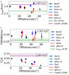 |
Fig. 3 VLSR, FWHM, and |

4 Column densities and gas temperatures
4.1 Radiative transfer modeling
The determination of the temperature and column densities of the targeted species is a first step to help us study the chemistry, and, therefore, evolutionary status of the cores. We estimated the column density of H2D+ and N2H+ and kinetic temperature toward all cores by modeling the velocity-integrated main beam temperature at the peak/central position using the non-LTE radiative transfer code RADEX (van der Tak et al. 2007). We assumed an isothermal homogeneous sphere. RADEX predicts the line intensities of the molecular transitions of interest for a given set of physical parameters: kinetic temperature, H2 density, molecular column density, Rayleigh-Jeans equivalent background temperature of a black body shaped radiation field (in this case, the cosmic microwave background (CMB) temperature of 2.73 K was adopted), and the observed line width. To convert to the main beam temperature, we adopted the main beam efficiency, ηmb, of 0.6 (ηα ∕ηmb ~ 0.8) measured by Buckle et al. (2009).
4.1.1 H2D+
The observed spatial distribution of the H2D+ emission is extended for all cores, and therefore the implicit assumption of unit beam filling factor is proper. The most recent available collisional properties of the H –H2 system and all its isotopic variations were studied and presented in Hugo et al. (2009). To determine the excitation of H2D+, we adopted the rates presented in Hugo et al. (2009) with two simplifications. First, our calculations only consider the lowest two energy levels of o-H2D+, the 111 ground state, and the 110 excited state which lies 17 K above the ground. This two-level approximation is valid at the low temperatures of prestellar cores (T ~ 10 K), and therefore for the present sample, since the next highest level, 212, lies at 109 K above the ground and its excitation is therefore negligible. The second simplification is that our calculations ignore reactive collisions. We note that in general the collisions between H
 and H2 may lead to reaction (i.e., the fully elastic case), excitation (i.e., the fully inelastic case), or both. Our assumption is justified by the work of Hugo et al. (2009), who show that at the low temperatures of interest here, the reactive collision rates are factors > 100 lower than the inelastic ones.
Our calculations include inelastic collisions of o-H2D+ with o-H2 and p-H2. Since we are dealing with very low temperatures, the ortho-to-para ratio of H2 is assumed to be equal to its thermal value (~10−4 in our case) instead of the high-temperature limit of 3. In several previous studies (van der Tak et al. 2005; Vastel et al. 2006; Caselli et al. 2008), the H2D+ abundances toward the cores of our sample (when studied) were calculated using scaled radiative rates adopted by Black et al. (1990), and therefore the column densities and abundances derived in those studies should be updated with the most recent rates, as we did here.
Column density (Nmol) and gas kinetic temperature (TKIN) estimates for the adopted volume density ( ) at the central position of core using RADEX.
4.1.2 N2H+
In this work, we used the newest available collisional data of N2H+ (Lique et al. 2015). As opposed to former collisional data, where the collisional partner was Helium (He), the new ones are calculated based on collisions with the most abundant partner in the interstellar medium, which is H2, and are found to be significantly different (Lique et al. 2008).
4.2 RADEX results
Table 3 presents the adopted gas densities n(H2) of the cores along with their derived column densities (N(H2D+) and N(N2H+)), and derived temperatures (TKIN) at the central position of each core. The average volume density, at least at the core center where we are focusing in this part of the analysis, was adopted as the values presented in Caselli et al. (2008). In particular for this sample, we report low kinetic temperatures between 6 and 9 K, and column densities for both species lying within the range of 0.4–2 × 1013 cm−2. The derived kinetic temperatures are used to assess the line thermal broadening per core presented in Sect. 3.2.
Comparing our observables with those presented in Caselli et al. (2008), we see that the reported Tmb values are similar in both studies, which indicates that the difference in beam size between JCMT and CSO plays a minor role, supporting our conclusion that the emission is extended and the beam is filled. The line widths are also similar except for L1521f and L1544. The observed difference is likely due to the more limited spectral resolution of the CSO backends. The column densities among the studies are consistent (mostly within a factor of 2), given the differences in adopted kinetic temperatures (up to 3 K), observed line fluxes, and molecular data. Increasing the number of observed transitions per species, and at multiple offsets, would allow the accurate determination of the kinetic gas temperature, column, and volume density, and the production of the column and gas kinetic temperature maps of the cores.
5 Modeling the spatial distribution of H2D+ and N2H+
A primary goal of this paper is to distinguish between dynamical models that turn a prestellar core into a protostar that have been proposed in the literature. To do so, we modeled the spatial distribution and line profiles of H2D+ and N2H+ (detected toward only two cores) for each core, as predicted from each dynamical model using advanced radiative transfer modeling, and compare the predicted emission with our observed maps.
5.1 RATRAN: initializing the model
To model the spatial distribution and line profiles of H2D+ and N2H+ (where present) emission from the cores, we ran the Monte Carlo radiative transfer code RATRAN (Hogerheijde & van der Tak 2000). RATRAN calculates synthetic line emission for the species of interest, taking into account the temperature and density gradients of the source, the dust emission and absorption properties, and the small-scale (e.g., thermal motions, turbulence) and large-scale (e.g., infall motions) source kinematics. We fix the physical structure of the sources by adopting the corresponding predicted temperature, density, and velocity structure from proposed dynamical models in the literature. The dynamical models examined in this study are described in Sect. 5.2. For our models, we assumed that the dust temperature is equal to the gas temperature, which is valid for environments of high volume density (>104 cm−3), and a gas-to-dust ratio of 100.
For our calculations, and to simulate the 2′ × 2′ observations, we defined a grid of 13 logarithmically spaced shells for each core, extending to an outer radius of 10 000 au for all cores except L694-2, which was extended to 15 000 au due to its larger distance (see Table 1). The density and velocity structures are shown in Fig. 8 and were adopted by Keto et al. (2015) for the different models which are described in more detail in Sects. 5.2.1–5.2.3.
The temperature profiles were adopted from the literature (L183, L694-2, L1517B, L1544, L1521f Pagani et al. 2007; Redaelli et al. 2018; Maret et al. 2013; Chacón-Tanarro et al. 2019; Crapsi et al. 2004). These profiles were derived using radiative transfer models to fit the observed gas (e.g., N2H+) or dust emission (e.g., mm IRAM observations), and are specific for each core. The LP and SIS models are by definition isothermal, while the QE-BES model predicts a range of temperatures, and is more consistent with the observed temperature variations (~5 K). Our approach to adopting the same temperature profile in all dynamical models may affect the brightness of the line, but not the dynamics (Keto & Caselli 2010). In this study, we examined the line morphology, which is highly dependent on the dynamics, meaning, the distribution of the velocities of the gas, rather than the small variations in the gas kinetic temperature; therefore, our general conclusions are robust.
The Doppler parameter, b, was calculated for each shell as equal to 0.6 × FWHM, where FWHM is the result of the Gaussian fitting process for each core and position presented in Table 2. In Table 4, we present the initial abundance profiles adopted during the modeling process for H2D+ and N2H+ for each core with the associated references, and the relevant modifications per model to achieve a good fit. In particular, we proceed to a more accurate determination of the abundance profiles by fitting the emission at the central position and expand the solution to the entire map (see Sect. 5.3). Lastly, to compare the modeled emission with observations, the resulting modeled spatial distribution is convolved to the beam size of the JCMT (14′′ at 372 GHz).
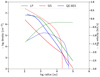 |
Fig. 8 Density (solid line) and velocity (dashed line) profiles of a prestellar core predicted by thethree dynamical models: LP flow (green), SIS (red), and QE-BES (blue), as presented in Keto et al. (2015). Each of the modeled profiles was adopted to model the H2D+ emission using RATRAN. |
5.2 Physical structure: dynamical models
Multiple hypotheses exist about the dynamical processes that take place for a prestellar core to collapse. To date, the determination of the most accurate model has been challenging. In this study, we examined three different dynamical models based on spherical symmetry that result in similar density profiles but very different velocity profiles across the cores. These models are the QE contraction of a BES, the LP flow (LP), and the inside-out collapse of the SIS.
We note that despite the similarity of the slopes in the density distribution, the different density profiles account for a total cloud mass of ~ 10 M⊙ for the QE-BES model, ~ 27 M⊙ for the LP model, and ~4 M⊙ for the SIS model, for a radius up to 30 000 au. Based on mass estimations alone, the SIS and QE-BES models appear to be the most suitable in reproducing the estimated mass for the cores in our sample (based on dust continuum observations; see Table 1). Here, we investigate the behavior of the gas. The quite distinct velocity profiles resulting from the different dynamical models are shown in Fig. 8. Gas emission observations in the optically thin regime that can trace those kinematics are therefore crucial. The models of interest are described below.
H2D+ and N2H+ abundances estimated with RATRAN for each core based on the JCMT observations.
5.2.1 LP flow
Larson (1969) attempted to solve numerically the dynamical equations concerning the collapse of a spherically symmetric isothermal core, known as Larson core, which is gravitationally unstable, yet all rotational, magnetic, and turbulent motions are neglected (free-fall collapse). The collapse, in this case, is nonhomologous, with the central region collapsing to a high density and reaching hydrostatic equilibrium and the outer regions collapsing to a much lesser extent, creating a first hydrostatic core object. In the meantime, Penston (1969) presented the dynamics of self-gravitating gaseous spheres, focusing on the isothermal case, which collapses in free-fall. The analytical solutions to the equations of free-fall collapse are used to produce the various symmetries (including spherical) at the instant when a dense hydrostatic object forms in the innermost dense regions of the core. For the hydrodynamic simulations, the diffusion approximation for radiative transfer was used.
The density and velocity profiles of the LP model (Fig. 8) were adopted by Keto et al. (2015), and are products of integrating Eqs. (11) and (12) in Shu (1977). To produce a similar density profile (slope ~ r−2) for all models (LP, SIS, QE-BES), the sound speed was 0.2 km s−1 at ~11 K, and the evolutionarytime was 2.8 × 10¹¹ s. The density follows a flat distribution with a central density n = 6.3 × 106 cm−3 out to ~850 au and follows an r−2 slope outward, with n = 3.5 × 104 cm−3 at ~ 10 000 au. The velocity gradually increases from 5 × 10⁻² km s−1 at 100 au, reaching a maximum of 10−1 km s−1 at ~850 au, where it reaches and remains at a constant velocity through to the outermost regions of the core.
5.2.2 SIS
Shu (1977) proposed the SIS model to describe the gravitational collapse of isothermal gas clouds. In this case, the collapse occurs from the inside out, with the inner and outer envelopes modeled separately. The inner envelope is assumed to collapse under free-fall conditions while the outer envelope is modeled as essentially static. The proposed density distribution in this case follows the r−3∕2 for the inner envelope, and r−2 for the outer envelope, adopting a sound speed, α = 0.2 km s−1 at ~11 K, and an evolutionary time t = ~2.5 × 10⁵ yr. In particular, the inner density is 2.5 × 106 cm−3 at 100 au, decreasing down to 1.4 × 104 cm−3 at ~10 000 au. The velocity profile in this dynamical model is characterized by a higher velocity at the center of the core (compared to the other dynamical models) of ~4 km s−1 at ~100 au and decreases down to 0.5 km s−1 at ~10 000 au, before starting to behave as a static sphere without infall in the outer parts of the core.
5.2.3 QE-BES
This model treats the prestellar core as a BES undergoing quasi-static contraction, in which the pressure in the system remains uniform and constant, due to a low rate of volume change. The pressure is not affected by small oscillations connected with small-scale processes within or near the cores. The notion of a BES was originally put forward in 1956 when it wasshown that an isothermal sphere of gas in an external pressurized medium has a critical size above which it is gravitationally unstable (Bonnor 1956; Ebert 1957). This model predicts a density profile following r−2 in the outer region of the core with an approximately constant density inward (e.g., Keto & Caselli 2010). The central density in this case is n = 107 cm−3 (Keto et al. 2015). The velocity profile predicted by this contraction model shows a so-called Λ-shape, starting from 0 km s−1 in the center (<100 au) and increasing outward, while reaching a maximum value (~1 km s−1) near the characteristic radius, rf, (~1000 au in this case), where we observe the transition from a constant/flat density distribution to that of r−2. After the velocity reaches its maximum value, it decreases again when moving toward the edge of the core.
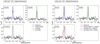 |
Fig. 9 Example of the abundance profile adjustment during the fitting process. The observed line profiles of H2D+ are overplotted with the modeled ones using RATRAN toward the central position of the L183 core. Three different dynamical models were adopted, QE-BES, SIS and LP flow. The original abundance profiles (left panel) were adopted by Pagani et al. (2009) and cannot reproduce the central peak of the observations. Adjusting the H2D+ abundance profile by applying a multiplication factor, resulted in a better reproduction of the observations for the LP and QE-BES models, while the SIS model failed to match the shape of the observed line profile. |
5.3 Abundances
Before determining the most representative dynamical model per source, we proceed with fine-tuning the abundance profiles of H2D+ and N2H+.
5.3.1 Abundance derivation: dynamical approach
We started the fitting process by adopting an abundance profile for the observed H2D+ per core from the literature and proceed to a more accurate determination of the abundance profiles by fitting the line emission at the central position for each core. To do so, we let the abundance vary by up to 2 orders of magnitude higher and lower from the initial abundance and using a step of a factor of 2. Table 4 lists the initial H2D+ abundance profiles adopted from the literature with their associated references and the multiplication factor we applied in this study to fit the peak line intensity of the central position. A constant abundance profile was also tested toward these cores but without resulting in a qualitative change on the results. Therefore, we adopted the more detailed abundance profiles when available throughout the paper. We note that for two cores, L694-2 and L1517B, initial abundance profiles could not be retrieved from the literature; therefore, we assumed a constant initial abundance of 1 × 10⁻¹⁰ which we varied as described above. Figure 9 shows an example of the fitting process toward L183.
Our observations concern only single transitions of both H2D+ and N2H+, while the physical structure is fixed. Therefore, although our fitting process results in an uncertainty of ~14%-18% (~3 ) for the derived abundances, this process somewhat underestimates the real uncertainties. Once we find the abundance profile that can reproduce the observed line profile in the central position of the core, we expand the solution to the entire map. In Table 5, we present the resulting optical depth for each line per model toward the central positions of each core. We find that the emission from both H2D+ 110 –111 and N2H+ 4–3 is mostly in the optically thin regime (τ < 1) justifying their good performance in tracing the dynamics of the cores.
5.3.2 Static sphere
To provide an independent determination of the abundances, we proceed with applying the same radiative transfer technique, but this time weadopted the physical structure of each source based on their previous dust and gas observations. In this case we assumed a static envelope, without infall or expansion motions. The temperature and density profiles were adopted from the literature (L183, L694-2, L1517B, L1544, L1521f Pagani et al. 2007; Redaelli et al. 2018; Maret et al. 2013; Chacón-Tanarro et al. 2019; Crapsi et al. 2004), and are based on continuum and gas observations, and they are, therefore, unique to each core. Again, the basic assumptions for all cores are that the gas and dust are thermally coupled, their temperatures are therefore set to be equal, and the gas to dust ratio is 100. As before, we defined a grid of 13 logarithmically spaced shells for each core, while the density and temperature profiles per core are described as follows.
Optical depth, τ, of H2D+ and N2H+ estimated with RATRAN at the central position of each core.
L183
For this core, we adopted the density and temperature profiles presented in Pagani et al. (2007), and are based on a detailed 1D radiative transfer modeling to fit both N2H+ and N2D+ emission (IRAM-30m cut observations), consistently with the dust emission (MAMBO; Pagani et al. 2004). In particular, the density profile follows a broken power law with an inner density ρ0 = 2.34 × 106 cm−3, with the density proportional to r−1 for a radius up to ~4000 au, and to r−2 for the rest of the core. The temperature profile has a constant value of 7 K up to 5600 au and increases outward up to 12 K.
L694-2
For this core, we adopted the density and temperature profiles presented in Redaelli et al. (2018). According to Arzoumanian et al. (2011), the density profile is given by:
![Mathematical equation: \begin{equation*} \rho(r)\,{=}\,\left[\frac{\rho_0}{1+\left(\frac{r}{r_0}\right)^2}\right]^{\frac{p}{2}}\end{equation*}](/articles/aa/full_html/2020/11/aa38457-20/aa38457-20-eq21.png) (6)
(6)
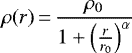
which Redaelli et al. (2018) adjusted for L694-2 to fit its observed Herschel/SPIRE dust continuum at 250, 350, and 500 μm, using radiative transfer modeling. In particular, the inner density ρ0 = 1.8 × 105 cm−3, the half maximum density radius r0 = 2500 au, and p = 3.3. The temperature profile is 8 K in the center of the core and increases outward to 12 K.
L1517B
Here, we adopted the density and temperature profiles presented in Maret et al. (2013) and Tafalla et al. (2004), respectively, based on radiative transfer modeling of the 1.2 mm continuum emission. In particular, the density profile of L1517B follows the form:
 (7)
(7)
with a ρ0 = 2.2 × 105 cm−3, a half maximum density radius r0 = 4.9 × 10³ au, and α = 2.5. The temperature profile is also taken from those studies and is assumed to be isothermal and equal to 10 K throughout the core.
L1544
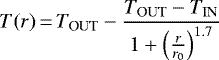
For this core, we adopted the most recent density and temperature profiles presented in Chacón-Tanarro et al. (2019), based on fitting the 1.1 and 3.3 mm continuum emission. The temperature profile follows the form:
 (8)
(8)
with outer temperature TOUT = 12 K, inner temperature TIN = 6.9 K, and critical radius r0 = 28.07″. The densityprofile follows the same form as in Eq. (7), but for ρ0 = 1.6 × 106 cm−3, a half maximum density radius r0 = 17.3″, and α = 2.6.
L1521f
For L1521f, we adopted the density and temperature profiles presented in Crapsi et al. (2004). In particular, the density profile follows the same form as in Eq. (7), but for a central density ρ0 = 1 × 106 cm−3, a half maximum density radius r0 = 2800 au, and α = 2, while the temperature is assumed to be isothermal and equal to 10 K for the entire core.
5.3.3 Abundance derivation: static approach
We find that the initial abundance profiles reproduce the line strength of the central peak position, requiring no modification for L183 and L1521f, and a modification of a factor between 0.8 and 4 for the H2D+ and N2H+ emission, respectively, toward L1544. The static model performs well in reproducing the central peak for all cores with minimum modification of the initial abundance profile. Therefore, we consider the H2D+ abundance determination to be more accurate compared to the one derived from the dynamical models toward the two cores for which we did not have prior knowledge of the H2D+ abundance. Our best fit results in [H2D+] of 2.5 × 10⁻¹⁰ for L694-2 and 1.5 × 10⁻¹⁰ for L1517B, and similar (within a factor of 2) to what was previously found for the rest of the cores. These results are summarized in Table 4.
5.4 RATRAN: results
In Figs. 10–16, we present the azimuthally averaged observed and modeled emission of H2D+ toward the cores for the different physical and kinematic structures predicted by the three dynamical models, LP, SIS, and QE-BES, and the static model. The corresponding plots using the original, before azimuthal averaging, maps of each core can be found in Appendix B. The synthetic spectrum is compared to the observed one at each map position using a simple χ2 approximation given by:
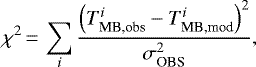 (9)
(9)
where  is the observed main beam temperatureper velocity channel (i),
  is the modeled one, and σOBS is the observed rms.
5.4.1 Individual cores
L183
For L183, as seen in Figs. 10 and B.1, the static, QE-BES and LP models all can reproduce the central (0″, 0″) observed peak intensity and line shape with <5% deviation. This similarity is easily justified since the abundance profiles are adjusted accordingly in order to fit the central position. The SIS model, however, predicts ~2 times larger line widths than observed, resulting in an order of magnitude larger χ2 (~900) compared to the rest of the models and demonstrating the poor quality of the fit produced by this model.
Moving outward, we see at 15″ offsets, that the LP model performs better in reproducing the observed peak intensities with absolute deviations of 10–30%, followed by both the static and QE-BES models with absolute deviations of 30–50%. The SIS model is again significantly worse (>3 times higher χ2 compared to the other three models) in reproducing the shape and intensity of the observed line profiles. At 30″ offsets, the LP model is still superior to the other models with typical deviations of ~15% from the observed emission, which is significantly closer to the observations compared to QE-BES and static models that show >40% deviations. The exception to this rule is the 30″ north, where all models underestimate the emission by 50–65%. Similarly, all models underestimate the observed emission by 50–90% at 45′′ offsets northward (both east, west, and center). On the other hand, at 45′′ offsets southward, the core is characterized by weaker emission and the LP model can reproduce reasonably well the observations (<15% deviations), which is indicative of a diversion from the spherical symmetry assumption (see Fig. B.1). We note that Pagani et al. (2007) did not report such diversions for other species (e.g., N2D+), but in that paper only the west–east cut is presented. Noticeably, the QE-BES model performs better than the static sphere at the larger offsets.
We conclude that the LP model performs better in reproducing the observed line profiles and intensities globally for L183, followed by the QE-BES model, while the static model significantly underestimates the emission toward the outer parts of the core. The SIS model cannot reproduce the intensity and morphology of the line profiles globally, and therefore it is the least suitable among the models.
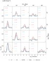 |
Fig. 10 Observed azimuthally averaged line profiles for each position of H2D+ maps toward L183, overplotted with the modeled ones for Static, LP, SIS and QE-BES models from RATRAN. |
L694-2
For L694-2, as seen in Figs. 11 and B.2, the static model reproduces the central (0″, 0″) observed peak intensity and line shape with only 1% deviation, followed by the LP model with <10% deviation. While the QE-BES model can also fairly reproduce the central emission, the SIS model fails to match the observations by producing a line profile with much stronger line wings than the observed, resulting in a χ2 >1000, which is two orders of magnitude higher than the LP and static models.
Interestingly, when we examine the modeled versus the observed emission globally, we see that the LP, QE-BES and static models can all reproduce the observed peak intensities equally well with absolute deviations of 2–12% at 15″ north–east and south–west from the central peak, while all three underestimate the observed line intensity at 15″ south–east and north–west by 30–50%. The SIS model reproduces neither the strength nor the shape of the lines at those offsets. At offsets >30″, the QE-BES model predicts emission that is 30–60% higher compared to the other models. This weak emission, however, is mostly within the rms limits, and therefore not possible to validate with the dataset in hand.
We conclude that for L694-2 we cannot clearly distinguish between LP, QE-BES, and the static models, as their predicted emission is very similar (mostly similar resulting χ2). Future deeper observations toward the outer parts of the core (e.g., >30″) will reveal if there is a weak emission similar to what the QE-BES model predicts, which will allow us to tell those models apart. The SIS model appears to be the least suitable among the models, failing to reproduce both the intensity and the shape of the line profiles globally.
L1517b
For L1517B, as seen in Figs. 12 and B.3, all three QE-BES, LP, and static models can reproduce the central (0″, 0″) observed peak intensity and line profile with <5% deviation, while the SIS model predicts ~15% lower intensity at the source velocity.
When we examine the modeled versus the observed emission globally, we see that both the LP and the static modelcan reproduce the observed peak intensities with absolute deviations of 0.5–8% at offsets within 15″, where the detections are more apparent, while the deviations of the models are >30% at larger offsets where the observed emission gets weaker. For the same grid of offsets, the QE-BES model does not performas well, showing larger deviations of 25–75%, with the only exception toward the central position (0″, 0″). Lastly, the SIS model appears to reproduce the peak intensities with deviations of 5–30% for within 15″, while it gets significantly worse at larger offsets (up to 80% for >30″). When we look at the line profile of the modeled emission though, it becomes apparent that the SIS model fails to reproduce the observed emission globally. The unsuitability is reflected in high χ2 at most positions that are about an order of magnitude higher compared to those of the other three models at the same offsets (Fig. 12). At offsets with no detected emission (most offsets >30″), all four models predict some weak emission within the rms limits, which cannot be directly addressed in the current paper. Future observations of higher sensitivity will be able to reveal such emission.
We conclude that for L1517B, both the static and LP models are able to reproduce the observed peak intensities, line profiles, and spatial distribution of the emission equally well, and therefore we cannot clearly discriminate them. The QE-BES model underestimates the emission at most offsets for >50%, while the SIS appears to be the least suitable among the models, and therefore can be safely excluded.
L1544
As seen in Figs. 13 and B.4 for L1544, both the QE-BES and LP models can reproduce the central (0″, 0″) observed peak intensity of H2D+ and line profile with <3% deviation, followed by the static model (~8%), while the SIS model predicts ~55% lower intensity at the source velocity.
When we examine the modeled versus the observed emission globally, we see that the LP model performs better in reproducing the observed peak intensities of detected emission with absolute deviations of 3–23% at offsets within 30″. For the same grid of offsets, the QE-BES model is the next most suitable model showing deviations of 0.1–52%, with the 0.1% only toward the central position (0″, 0″), followed by the static model with deviations of 8–70%. Lastly, the SIS model does a fairly good job in reproducing the peak intensities with deviations of 2–50%. When we examine the line shape (profile and spatial distribution) of the modeled emission though, it becomes apparent that the SIS model fails to reproduce the observations globally. This failure is clearly depicted by the resulting χ2, which accounts for all velocity channels of the emission (not just the central peak), and is found to be systematically and significantly higher than the rest of the models at most positions where emission is present (e.g., up to 1000 at 0″ offset, compared to <100 for the rest of the models; Fig. 13). The situation is different at offsets with no detected emission (i.e., most offsets >45″), where the static model is the only one to predict no emission, while all dynamical models predict weak emission but mostly within the rms limits. This discrepancy can be addressed in the future by obtaining higher sensitivity observations, which can reveal the predicted weak emission of the dynamical models. If the static model predictions are correct and there is indeed no emission toward the outer parts of the core, this result can be explained by the more realistic approach on density and temperature profiles, for this core, which are based on dust observations and not simulations.
The situation is less clear when simulating the N2H+ 4–3 emission. As we see in Figs. 14 and B.5, all models apart from the SIS model can reproduce the observed peak intensity and line profile at the (0″, 0″) and (15″, 15″) offsets (where emission is present). The QE-BES model is also tested by Redaelli et al. (2019) toward L1544, and is found to reproduce the N2H+ 1–0 and 3–2transitions at the central dust peak position reasonably well. All models in our study systematically and significantly overestimate the emission by an order of magnitude at all other inner positions and at offsets of 30″ regardless of the direction. Therefore, no model is able to explain the observed N2H+ 4–3 spatial distribution toward L1544 globally. We conclude that the LP model performs better in reproducing the observed line profiles and intensities of H2D+ globally for L1544, while the SIS model appears to be the least suitable among the models.
L1521f
For this core, as seen in Figs. 15 and B.6, both QE-BES and LP models can reproduce the central (0″, 0″) observed peak intensity and line profile of H2D+ with <12% deviation, followed by the static model (~17%), while the SIS model predicts ~75% lower intensity at the source velocity.
When we examine the modeled versus the observed emission globally, we see that apart from two offsets at (0″, 0″) and (−15″, −15″), where the LP, QE-BES, and static models can reproduce the observed peak intensity similarly and with <35% deviations, they systematically and significantly underestimate the peak intensity between 52% and 96% at the rest of the offsets with detections. The SIS is the only model providing a good representation of the observed peak intensity for the majority of offsets within 45″ from the center, with deviations of 8–40%. Nevertheless, similarly to the other cores, the SIS model fails to reproduce the line profiles resulting in very high χ2 (>100), when all velocity channels are taken into account (Fig. 15). The exceptions to this trend are the two observed offsets at 45″ north, where the SIS model appears to be the only one to predict the observed emission.
When we examine the N2H+ emission in Figs. 16 and B.7 we see that all models apart from the SIS model can reproduce the central peak emission within 10%, but overestimate the emission at 15″ offsets by >60%, while they are all consistent with showing no emission at larger offsets (>30″). The amount of available information connected to N2H+ is not sufficient to draw clear conclusions.
We find that none of the models perform well in reproducing the observed emission globally, both line profiles, and the intensity and distribution of H2D+, toward L1521f. This outcome may be due to the fact that L1521f is a more evolved (protostellar) object compared to the rest of the sample of prestellar cores, and therefore it is characterized by more complex dynamics and physical structure. Protostellar cores, for example, are known to drive powerful outflows, and therefore the tested dynamical models that account only for infall motions may not be expected to reproduce the observations consistently with what we see. The situation is similar for the model of the static envelope. The good quality fit of the SIS model at the reported offsets may indicate that the dynamical evolution from a prestellar to a protostellar core is better represented by the SIS model rather than the LP model in opposition to what we see for prestellar cores. Given the poor ability of the model to reproduce the emission at a more global scale,however, we consider this alignment to be rather coincidental. The less problematic fit we get toward N2H+ indicates that H2D+ is dynamically decoupled from N2H+, with the former requiring a more complex structure.
5.4.2 Summary of RATRAN results
We find that the LP flow can reproduce the observed line profile and intensity of H2D+ fairly well on a global scale (most offsets), and appears to be superior to the static, SIS, and QE-BES models for two out of the four prestellar cores, L183 and L1544. The influence of the abundance profiles on the simulated line intensity makes clear differentiation among those models challenging. For L1517B, the situation is less clear, with the static sphere reproducing the observationsequally as well as the LP model. For L694-2, we cannot clearly distinguish between the LP, QE-BES, and static sphere models. On the other hand, all models fail to reproduce the observed line profiles and distribution of H2D+ toward the protostellar core L1521f, indicating that the predicted model dynamics taking place during the prestellar phase are not suitable for a more evolved object, where outflows and a central heating source are present. These findings are summarized in Fig. 17 at offsets along a cut in the south–west/north–east direction.
In addition, our modeling clearly demonstrates that the SIS dynamical model fails to reproduce the observed line profile for all cores, independentof the initial abundances. While the density profile of the SIS model shows a similar slope to the other two models (all models follow ~ 1/r2 profile), the exact density profile results in a smaller mass in the same volume of gas compared to the other two dynamical models. As a result, the overall density distribution of the SIS model is not sufficient to excite the H2D+ transition inthe amount required to match the observations. This behavior is clearly seen in the abundance calculations, where we find the H2D+ abundance needs to be 2–4 orders of magnitude higher for the SIS model compared to the other two models for all sources. The observed differences on the abundances can be depicted in the resulting column densities as well. For a given volume density an increase of a factor of 100 in the abundance corresponds to an increase in the molecular density by the same factor. For example, in the case of the H2D+ emission toward L1544 the LP model results in a column density of 1.6 × 1013 cm−2, while the SIS model results in a column density of 3.2 × 1015 cm−2. Referring back to the RADEX analysis (Sect. 4.2), we find N(H2D+) = 2.0 × 1013 cm−2, which is in very good agreement with the LP model but 2 orders of magnitude lower than the column density from the SIS model. This result demonstrates once more the poor performance of the SIS model compared to the LP and QE-BES models.
Moreover, the QE-BES model gives a core mass of ~10 M⊙, the LP model of ~ 27 M⊙ and the SIS model of 4 M⊙, while the masses of the cores derived from dust emission are 4–10 M⊙. We conclude that the differences in the modeled versus observed masses affect our abundance determinations, resulting in higher or lower H2D+ abundance depending on whether the modeled mass for a defined volume is higher or lower, respectively, than observed. To examine the effects of the assumed mass in the reproduction of the observations we notice that L1517B is as massive as 4 M⊙ (i.e., the same mass as the SIS model has), but the SIS model still fails to reproduce the observations; therefore, our conclusion on excluding the SIS model as a possible dynamical model to explain the observed H2D+ emission is independent from the mass assumptions. Similarly, the LP model has a mass ~3 times higher than the core masses in our sample, yet it is able to reproduce the observations at all prestellar cores. We therefore conclude that although the mass differences introduce higher uncertainties in the abundance determinations, they do not affect the line profiles. The line profiles depend on the velocity structure of the models, making our analysis and conclusions in differentiating between the dynamical models robust. Referring to the results presented in Sect. 3.2, we found that there are significant nonthermal contributions toward all cores, which are traditionally attributed to turbulence and magnetic pressure. The ability of the LP flow to reproduce the observations without taking those phenomena into account, unlike the adopted QE-BES model (i.e., turbulence), indicates that they are not significant in driving the core dynamics.
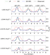 |
Fig. 17 Observed line profiles of H2D+, overplottedwith the modeled ones for LP, SIS, and QE-BES models from RATRAN at selected offsets: (0″, 0″), (15″, 15″), and (−15″, −15″). |
6 Discussion
In this section, we discuss the main findings of this paper. In particular, we attempt to explain the observed line broadening, the presence of N2H+ toward only two of the five cores in our sample, and, lastly, the core collapse dynamics, which is a debatable topic both in theory and observations.
6.1 Line broadening
We first discuss our results from the line profile analysis presented in Sect. 3.2. We find that the line width of both N2H+ and H2D+ cannot be explained by thermal broadening alone, and the nonthermal contributions are variable with offsets and overall higher for N2H+ than H2D+ (Sect. 3.2). The observed variations with offsets of the nonthermal contributions are as high as ~ 130% and beyond the uncertainties. Traditionally, nonthermal motions are explained by presence of magnetic pressure or turbulence. In this study, we show that the LP flow can reproduce the line width of the H2D+ observationsin multiple offset locations (e.g., see Fig. 10), which by definition (free-fall) does not take into account turbulence or magnetic fields; therefore, the nonthermal broadening can be merely due to infall/compression motions, characteristic of the dynamical structure of prestellar cores.
6.2 N2H+ 4–3 emission as an evolution tracer
Here, we discuss the origin of the N2H+ 4–3 emission. We detect the N2H+ 4–3 transition toward two out of the five cores in our sample, in contrast to the ground ortho-H2D+ 110 –111 emission which is present toward all cores. In addition, H2D+ is more spatially extended than N2H+, which is traced only within 15′′ of the core centers.
To understand the spatial differences, and the presence or absence of these species toward these cores, we considered the critical densities of the observed transitions, calculated based on the available molecular data. In particular, the observed ortho-H2D+ 110 –111 at 372.4 GHz is characterized by a critical density ncr = 1.2 × 105 cm−3 at 10 K, while the observed N2H+ 4–3 transition at 372.67 GHz is characterized by a critical density ncr = 7.7 × 106 cm−3 at 10 K, which is more than an order of magnitude higher. We also note that the N2H+ 1–0 transition at 93.17 GHz, which has a comparable critical density to the ground H2D+ transition (ncr ~ 1.4 × 105 cm−3 at 10 K), has been previously detected toward all cores in our sample (Crapsi et al. 2005). We conclude that the observed spatial differences between the two species are due to the higher densities traced by N2H+ 4–3, which are unsurprisingly located toward the more central regions of the cores (see, e.g., density profiles in Sect. 5.3.2). Indeed, this interpretation is supported by the observed lower J transitions 3-2 and 1–0 of N2H+ toward L1544 (Redaelli et al. 2019), which are found to be up to a factor of four more extended compared to the 4–3 transition.
The absence of N2H+ 4–3 emission for L694-2 and L1517B can be explained by their lower central densities on the order of ~105 cm−3, namely, an order of magnitude lower than the critical density of N2H+ 4–3. Similarly, the presence of this transition can be explained for L1521f and L1544, given their higher central densities of ~106 cm−3. Along this line of reasoning, the non-detection of N2H+ 4–3 toward L183 is more puzzling, given that its central density is found to be similar to those of L1521f and L1544, indicating that its central density may be overestimated.
We conclude that N2H+ 4–3 could be used as a chemical clock, in the sense that it traces a fairly high density environment achievable only in more evolved prestellar/early protostellar core phases. Our conclusion is supported by the presence of this emission toward the only protostellar (more evolved) core in our sample (L1521f). This approach would mean that L694-2 and L1517B are less-evolved cores.
6.3 Differentiating between the theories of collapse
Here, we discuss our findings from the RATRAN analysis presented in Sect. 5, where we compare the performance of the different dynamical models of collapse. We find that the LP model can mostly reproduce the observed line profiles and spatial distribution of H2D+, followed in suitability by the QE-BES model. Meanwhile, the SIS model fails to reproduce the line width globally, predicting a very prominent double peak line profile toward the central position of all cores, in contrast to the observed single peak. Although the LP model seems to be superior to the QE-BES model for at least two of the prestellar cores in the sample, we cannot distinguish between the two models with high confidence. The widths of the line profiles can be mostly reproduced by both models, while in addition the emission resulting from adopting LP conditions is closer to the observed line intensity on a more global scale compared to the QE-BES model. All models fail to reproduce the emission from the one protostellar core in our sample, L1521f, which is indicative of the more complex structure of a protostellar object with respect to a prestellar core, namely, presence of winds and outflows, disk, internal radiation, different grain sizes, and chemistry.
The abundance profiles have a significant effect on the simulated line intensity. We consider the abundance derivation from the dynamical models to be less accurate compared to those of the static model, due to the differences in the total core mass that each model implies. As we explained in Sect. 5.4 the exact density distribution over a specific volume (i.e., different mass) affects the degree of excitation of H2D+ and therefore its line intensity. For example, to match the H2D+ line intensity of L1544 (~8 M⊙), the H2D+ abundance had to be lower in the case of the LP model (> 10 M⊙) compared to those of the QE-BES (~10 M⊙) or SIS (<10 M⊙) models. The static model, on the other hand, is based on continuum observations and therefore it accounts for the observed total mass of each individual core. Breaking the observed discrepancy between masses derived from continuum and gas observations will allow proper differentiation between the LP and QE-BES models. To achieve this goal, the dynamical models need to be “tailored” to match the observed mass per individual core. Such a procedure, however, requires prior knowledge of the exact evolutionary status of each core, and is beyond the scope of this work.
Unlike the line intensity, which in the optically thin regime (τ < 1; see Table 5) highly depends on the adopted abundances, the shape of the line profile for a given abundance profile depends mostly on the velocity structure, which is unique per dynamical model. Therefore, we can safely exclude the SIS model as a possible dynamic model to explain H2D+ emission for all cores. The situation is similar for N2H+, where present. Our qualitative results remain even when a constant abundance profile is adopted for each core.
To understand the differences in the shape of the line porofile between the dynamical models, we explore the physical location of the H2D+ emission and we compare it to other tracers from previous work. The observed 110 –111 ground-state transition of ortho-H2D+ at 372.4 GHz is characterized by a critical density ncr = 1.2 × 105 cm−3 at 10 K, serving as a rather dense gas tracer. Looking at Fig. 8, we see that in the case of the SIS model, the observed H2D+ transition would better probe the innermost regions (< 1000 au). In the case of the QE-BES and LP models, however, it traces a greater volume of the gas (<10 000 au), but not the outer layers up to 100 000 au. The obvious mismatch between the predicted and observed H2D+ line profiles produced assuming an SIS collapse suggests that high-velocity inflow in the inner parts of the cores fails to explain the H2D+ emission. The line profiles produced by the LP and QE-BES models can mostly reproduce the observed line profiles, suggesting that more moderate contraction motions in the inner regions are more applicable (e.g., by three orders of magnitude difference in velocity). Keto et al. (2015) performed a similar analysis for H2O and C18 O toward L1544 and found that the QE-BES model reproduces the shape and intensity of the line profiles for both species, while the LP model produced a more complex profile for the C18 O similar to what we see for H2D+ in the SIS model in this study. To understand better the observed differences in the line profiles produced from different models, we need to consider the origin of the emission. In particular, the C18 O transition presented in Keto et al. (2015) is characterized by a critical density about two orders of magnitude lower than that of the H2D+ line examined here. Therefore, it is better at tracing less dense gas compared to the ground H2D+ transition. Looking at Fig. 8, we see that the outer regions of the core in the LP hypothesis are characterized by much higher velocities, explaining the broad wings modeled in C18 O. In conclusion, the QE-BES model can explain the observed line profiles of C18 O, H2D+ and H2O, both in shape and intensity, for the central position of L1544, while the LP and SIS models cannot simultaneously explain the observed emission.
In addition, we examine the performance of the static sphere. We find that the static model, which is based on the continuum observations of each core, can also reproduce the observations fairly well and similarly to the LP model for at least one core (L 1517b), demonstrating the importance of the adopted abundance profiles. This model, however, does not take into account infall motions. With only a single available transition of H2D+, a more accurate determination of the abundance profile and its proper coupling to the specific core dynamics is very challenging.
We conclude that coupling gas core dynamics and chemistry with dust properties is crucial to differentiating between the QE-BES and LP models, and therefore, should be considered in future studies. In particular, chemical modeling is essential to constrain the chemical age of each core, which will subsequently lead to the coupling of the dynamical models to the observed mass of each individual core.
To be able to draw stronger conclusions it is necessary to expand this analysis to a larger sample of known prestellar and protostellar cores. If the LP model is confirmed toward a larger sample of cores, its specific initial conditions indicate that the prestellar cores may form by compression or accretion of gas from larger scales (>10 000 au). On the other hand, if the QE-BES model is confirmed, it means that quasi-hydrostatic cores can exist within turbulent ISM, which would be against predictions from numerical simulations (Tilley & Pudritz 2004).
7 Summary–conclusions
This paper presents an analysis of H2D+ 110 –111 and N2H+ 4–3 toward one protostellar and four prestellar cores using 2′ × 2′ maps from JCMT. We present a basic line analysis for all positions in the maps where emission is detected. We estimated the average physical conditions (TKIN and NCOL) toward the center of the cores using the non-LTE radiative transfer code, RADEX, incorporating the latest collisional data available for both species. The derived kinetic temperatures per core are used to assess the thermal contributions on the observed line widths. Finally, we tested three different dynamical scenarios, using the advanced radiative transfer code RATRAN to model the spatial distribution of the gas traced by the optically thin H2D+ 110 –111 and N2H+ 4–3 line emission and reproduce the sizes of the observed maps. The latter allowed us to not only test which of the available dynamical scenarios is the most favorable for the prestellar core phase but also to derive abundance profiles of the observed species. Our main conclusions are summarized as follows.
-
Thermal broadening alone is not sufficient to explain the line widths of H2D+ and N2H+ measured toward the majority of the positions in the maps with clear detections. This finding suggests that nonthermal effects play a significant role at the very early stages of star formation. The nonthermal contributions can be merely attributed to the infall/compression motions predicted by the LP flow. Therefore, in that scenario, turbulent and magnetic pressure contributions are not required to explain the observed line width.
-
The nonthermal contributions are generally found to be stronger in the innermost parts of L694-2 and L1544 (<15″; with the exceptions of few offsets which are similar) and are found to be higher for N2H+ than H2D+. We report variations to nonthermal contributions up to a factor of 2.5 at all cores for different offsets and beyond the uncertainties. The lack of sufficient N2H+ detections at offset positions does not allow a meaningful investigation on nonthermal variations with radius for that emission.
-
N2H+ 4–3 was only detected toward two of the cores, L1521f and L1544. Given that L1521f is known to be a VeLLO, and therefore more evolved than a prestellar core, and given that both cores are located at the same distance, these detections indicate that L1544 may also be more evolved compared to the rest of the sample. In that case, N2H+ 4–3 can be used as a chemical clock, tracing the higher densities achieved during core evolution.
-
The RADEX analysis results in similar mean column densities of H2D+ and N2H+ (~1013 cm−2) for L1521f and L1544.
-
The RATRAN analysis reveals that the LP flow is superior in reproducing the H2D+ spatial distribution and line profiles toward two of the prestellar cores, while for the other two it is followed by the QE-BESand static scenarios, without being able to differentiate clearly between those.
-
The SIS model fails to reproduce the shape and strength of the line profiles for the majority of the positions toward all cores and, therefore, does not appropriately describe the dynamical nature of these cores.
-
The RATRAN analysis reveals that none of the scenarios can reproduce the H2D+ emissiontoward the protostellar core, L1521f, indicating that more complex dynamical and chemical structures need to be considered, including outflow activity and radiation or wind pressure from the central heating source.
We explored the most prominent dynamical scenarios based on spherical contraction to explain the H2D+ and N2H+ (where present) emission toward four prestellar and one protostellar core. With the observations and sample in hand we cannot clearly differentiate between the LP flow and QE-BES models, but can clearly exclude the SIS model. Our conclusions remain consistent after adopting a jump-drop or a constant abundance profile. To differentiate between theother collapse scenarios is necessary to construct dynamical models adapted to the individual observed core mass. In addition, testing the models will benefit from transitions of more molecular species in both the optically thin and optically thick regimes (e.g., van der Tak et al. 2005) and a larger sample of cores. Such data will inform us if the gas collapses as a free-fall (LP) or if turbulence is indeed crucial for the gas dynamics of cores.
In future, non-spherical models, such as oblate ones resulting from ambipolar diffusion, should also be considered. Applying chemical modeling tailored to the physical structure of each source to fit the H2D+ and N2H+ observed abundances, will provide us with the age (e.g., Brünken et al. 2014) and therefore the evolutionary status of each core, allowing us to link the chemical to the dynamical evolution of prestellar cores overall. Lastly, high angular resolutions to reach the emission in the inner 100 au (e.g., ALMA) of the prestellar cores should prove to be a powerful tool to explore the gas dynamics, but the observed chemical inner holes toward those objects and the heavy freeze-out, make such observations very challenging.
Acknowledgements
We would like to thank the anonymous referee for providing helpful comments and suggestions that improved the paper. EK is funded by the STFC (ST/P00041X/1). We thank Tim van Kempen and Werner Salomons for useful contributions during data reduction and analysis.
Appendix A Line analysis per core
Our line profile findings per source are described as follows.
L183
For L183 (Fig. 3), the VLSR ranges between 2.25 ± 0.05 and 2.48 ± 0.04 km s−1, and within the upper and lower velocities reported by Ho et al. (1978) and Caselli et al. (2008). The fact that the measured VLSR is not constant but varies with offset indicates local changes in the global kinematics of the core. The FWHM ranges from 0.32 ± 0.08 km s−1 to 0.58 ± 0.07 km s−1. With the exception of only few offsets (>40′′ southwest and northwest), the observed FWHM cannot be explained by thermal broadening alone (beyond the errors). The FWHM is overall up to ~90% larger than that expected from thermal broadening alone. Lastly, the  varies between 0.12 ± 0.03 K and 0.48 ± 0.03 K, with the highest measurements found toward the center and a gradual decrease outward. The observed variations at similar offsets, as well as the fact that there is an increase in
  at the most outward position, can be explained by inhomogeneities present in the medium.
L694-2
The VLSR for L694-2 (see Fig. 4) ranges from 9.47 ± 0.04 km s−1 to 9.65 ± 0.03 km s−1. There is not a specific trend on the observed VLSR variations, but the difference of up to ~0.2 km s−1 indicates local kinematic differences throughout the core. In this case, the FWHM ranges from 0.39 ± 0.1 to 0.63 ± 0.09 km s−1. With the exception of a single offset at ~42′′, where thermal broadening alone can explain the observed FWHM, the nonthermal contributions are significant at all other offsets inward (< 40′′). The line is generally up to ~96% broader than expected from thermal broadening alone. The decreased FWHM at a larger offset, may indicate a decrease in nonthermal contributions at the outermost parts of the core. Finally, the  values gradually decrease with offset, with local variations in
  pointing toward medium inhomogeneities.
L1517B
If one compares Fig. 5 to Figs. 3–4, 6–7, it is noticeable that the H2D+ emission of L1517B is less spatially extended than seen toward the rest of the cores; Indeed, the line emission in this core is rather concentrated around the central position of the 850 μm dust peak (< 30′′). The VLSR of L1517B ranges from 5.73 ± 0.03 to 5.82 ± 0.03 km s−1, and decreases with increasing offset. The FWHM ranges from 0.36 ± 0.06 to 0.49 ± 0.06 km s−1. Thermal broadening alone can explain the observed FWHM at most offsets for core temperatures >10 K. This temperature is higher by a factor of 2 compared to the one we determined in Sect. 4.2 for thissource, but still within the acceptable temperature range of prestellar cores. The line is ~85% broader than expected from thermal broadening alone. Lastly, the  is once again the highest in the central position and decreases with increasing offset without signs of inhomogeneities.
L1544
The H2D+ analysis forthis source (Fig. 6) shows that the VLSR ranges between 7.07 ± 0.03 and 7.21 ± 0.02 km s−1, with a meanVLSR value of 7.15 ± 0.03 km s−1. All measurements are within the range previously reported by Ho et al. (1978) and Caselli et al. (2008). The FWHM ranges from 0.38 ± 0.07 to 0.61 ± 0.08 km s−1, which is systematically higher than the thermal broadening contributions (e.g., a mean value of 0.48 ± 0.07 km s−1 is ~40% higher). The observed widths are statistically larger than the expected thermal width in five different offsets, including the central position. As mentioned earlier, we attribute this difference to nonthermal contributions. With the exception of one offset at ~40′′ north, the nonthermal contributions are higher in the center compared to the rest of the offsets. The line is generally up to ~90% broader than expected from thermal broadening alone. Finally, the highest value of  (0.55 ± 0.02 K) is found in the central position, while it generally decreases with increasing offset. The fact that at certain offsets, the
  varies by a factor >2 and beyond the errors is indicative of local inhomogeneities in the medium (in density and/or temperature).
Given that N2H+ 4–3 emission was detected toward only two positions, we do not show a plot associated with its analysis but summarize our results as follows. The VLSR is found to be ~7.20 ± 0.04 km s−1, that is, within the uncertainties of the corresponding H2D+ value. As in the case of H2D+, thermal broadening does not fully account for the FWHM of N2H+ (0.4 ± 0.1 km s−1), as the observed FHWM is broader by a factor of ~4. In the case of N2H+, nonthermal widths are higher by at least a factor of ~2.5 compared to those of H2D+. Therefore, N2H+ emission appears to stem from a medium of higher nonthermal motions compared to H2D+ or that these mechanisms somehow affect N2H+ more. Finally, both detections of N2H+ have very low  values, with a maximum value of 0.12 ± 0.03 K, a factor of 5 lower than the H2D+ peak intensities.
L1521f
This core (see Fig. 7) is the only known protostellar core in the sample (Bourke et al. 2006) and the one out of two for which N2H+ 4–3 is detected. The line analysis of H2D+ is presented in Fig. 7. The VLSR ranges between 6.41 ± 0.02 and 6.54 ± 0.03 km s−1. The FWHM values range from 0.34 ± 0.05 to 0.55 ± 0.07 km s−1. The FWHM can be explained by thermal broadening at the central position and higher offsets (>30′′). At intermediate offsets (~20′′), however, the FWHM is up to a factor of 2 larger than that expected from thermal broadening. While magnetic and turbulent contributions are also likely to play a role toward this core, we recall that this core is at a later evolutionary state compared to the rest of the sample. Indeed, its known compact outflow (Takahashi et al. 2013) may also contribute to the observed line broadening, although H2D+ is not known to trace outflow activity.  fluctuates between 0.10 ± 0.02 and 0.30 ± 0.05 K without showing a specific trend. We attribute the observed variations to local changes in density and/or temperature (e.g., a clumpy medium; Tokuda et al. 2018).
As in L1544, N2H+ emission was detected toward only two positions, and therefore we do not show an associated offset plot. The VLSR took values of 6.47 ± 0.03 and 6.56 ± 0.04 km s−1, are again within the uncertainties of the corresponding H2D+ values. At the central position, the FWHM is 0.6 ± 0.1 km s−1, therefore broader by a factor of 5 compared to the width expected from thermal broadening. The nonthermal contributions decrease by 65% at the offset position. Therefore, the nonthermal effects are higher in the center of the core. This behavior is in contrast to what we saw in the H2D+ case, where the central position did not require nonthermal effects to explain the observed FWHM. Therefore, as in the case of L1544, the nonthermal contributions seem to have a more significant effect on N2H+ emission compared to H2D+ emission. In the case of L1521f, this behavior could indicate that N2H+ emission originates from outflow cavities, as opposed to H2D+ emission, or that the magnetic pressure and turbulence affect the two species differently. Finally, at the offset position, the measured  of the N2H+ line (0.30 ± 0.04 K) is very similar to that of the H2D+ line.
Appendix B RATRAN results: original dataset
In Figs. 10–16, we present the original, before azimuthal averaging, maps of H2D+ 110 –111 and N2H+ 4–3 toward the cores, overplotted with the modeled ones for Static, LP, SIS and QE-BES models from RATRAN.
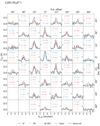 |
Fig. B.1 Observed line profiles before azimuthal averaging for each position of H2D+ maps toward L183, overplotted with the modeled ones for Static, LP, SIS and QE-BES models from RATRAN. |
References
- André, P. 2017, Comptes Rendus Geosci., 349, 187 [NASA ADS] [CrossRef] [Google Scholar]
- André, P., Men’shchikov, A., Bontemps, S., et al. 2010, A&A, 518, A102 [Google Scholar]
- Arzoumanian, D., André, P., Didelon, P., et al. 2011, A&A, 529, A6 [NASA ADS] [CrossRef] [EDP Sciences] [Google Scholar]
- Beichman, C. A., Myers, P. C., Emerson, J. P., et al. 1986, ApJ, 307, 337 [NASA ADS] [CrossRef] [Google Scholar]
- Bergin, E. A., & Tafalla, M. 2007, ARA&A, 45, 339 [NASA ADS] [CrossRef] [Google Scholar]
- Black, J. H., van Dishoeck, E. F., Willner, S. P., & Woods, R. C. 1990, ApJ, 358, 459 [NASA ADS] [CrossRef] [Google Scholar]
- Bonnor, W. B. 1956, MNRAS, 116, 351 [CrossRef] [Google Scholar]
- Bourke, T. L., Myers, P. C., Evans, Neal J., I., et al. 2006, ApJ, 649, L37 [NASA ADS] [CrossRef] [Google Scholar]
- Broderick, A. E., & Keto, E. 2010, ApJ, 721, 493 [NASA ADS] [CrossRef] [Google Scholar]
- Brünken, S., Sipilä, O., Chambers, E. T., et al. 2014, Nature, 516, 219 [NASA ADS] [CrossRef] [PubMed] [Google Scholar]
- Buckle, J. V., Hills, R. E., Smith, H., et al. 2009, MNRAS, 399, 1026 [NASA ADS] [CrossRef] [Google Scholar]
- Caselli, P., Benson, P. J., Myers, P. C., & Tafalla, M. 2002, ApJ, 572, 238 [NASA ADS] [CrossRef] [Google Scholar]
- Caselli, P., van der Tak, F. F. S., Ceccarelli, C., & Bacmann, A. 2003, A&A, 403, A37 [Google Scholar]
- Caselli, P., Vastel, C., Ceccarelli, C., et al. 2008, A&A, 492, 703 [NASA ADS] [CrossRef] [EDP Sciences] [Google Scholar]
- Caselli, P., Pineda, J. E., Zhao, B., et al. 2019, ApJ, 874, 89 [NASA ADS] [CrossRef] [Google Scholar]
- Chacón-Tanarro, A., Pineda, J. E., Caselli, P., et al. 2019, A&A, 623, A118 [NASA ADS] [CrossRef] [EDP Sciences] [Google Scholar]
- Crapsi, A., Caselli, P., Walmsley, C. M., et al. 2004, A&A, 420, 957 [NASA ADS] [CrossRef] [EDP Sciences] [Google Scholar]
- Crapsi, A., Caselli, P., Walmsley, C. M., et al. 2005, ApJ, 619, 379 [Google Scholar]
- Crapsi, A., Caselli, P., Walmsley, M. C., & Tafalla, M. 2007, A&A, 470, 221 [NASA ADS] [CrossRef] [EDP Sciences] [Google Scholar]
- Crutcher, R. M., Nutter, D. J., Ward-Thompson, D., & Kirk, J. M. 2004, ApJ, 600, 279 [NASA ADS] [CrossRef] [Google Scholar]
- Currie, M. J., Berry, D. S., Jenness, T., et al. 2014, ASP Conf. Ser., 485, 391 [Google Scholar]
- Di Francesco, J., Johnstone, D., Kirk, H., MacKenzie, T., & Ledwosinska, E. 2008, ApJS, 175, 277 [NASA ADS] [CrossRef] [Google Scholar]
- Ebert, R. 1957, ZAp, 42, 263 [Google Scholar]
- Enoch, M. L., Evans, Neal J., I., Sargent, A. I., et al. 2008, ApJ, 684, 1240 [NASA ADS] [CrossRef] [Google Scholar]
- Friesen, R. K., Di Francesco, J., Bourke, T. L., et al. 2014, ApJ, 797, 27 [NASA ADS] [CrossRef] [Google Scholar]
- Friesen, R. K., Pon, A., Bourke, T. L., et al. 2018, ApJ, 869, 158 [NASA ADS] [CrossRef] [Google Scholar]
- Fu, T.-M., Gao, Y., & Lou, Y.-Q. 2011, ApJ, 741, 113 [NASA ADS] [CrossRef] [Google Scholar]
- Goodman, A. A., Barranco, J. A., Wilner, D. J., & Heyer, M. H. 1998, ApJ, 504, 223 [NASA ADS] [CrossRef] [Google Scholar]
- Harju, J., Haikala, L. K., Lehtinen, K., et al. 2006, A&A, 454, L55 [NASA ADS] [CrossRef] [EDP Sciences] [Google Scholar]
- Ho, P. T. P., Martin, R. N., & Barrett, A. H. 1978, ApJ, 221, L117 [NASA ADS] [CrossRef] [Google Scholar]
- Hogerheijde, M. R., & van der Tak, F. F. S. 2000, A&A, 362, 697 [NASA ADS] [Google Scholar]
- Hugo, E., Asvany, O., & Schlemmer, S. 2009, J. Chem. Phys., 130, 164302 [NASA ADS] [CrossRef] [PubMed] [Google Scholar]
- Keto, E., & Caselli, P. 2008, ApJ, 683, 238 [NASA ADS] [CrossRef] [Google Scholar]
- Keto, E., & Caselli, P. 2010, MNRAS, 402, 1625 [NASA ADS] [CrossRef] [Google Scholar]
- Keto, E., Caselli, P., & Rawlings, J. 2015, MNRAS, 446, 3731 [NASA ADS] [CrossRef] [Google Scholar]
- Kirk, H., Dunham, M. M., Di Francesco, J., et al. 2017, ApJ, 838, 114 [CrossRef] [Google Scholar]
- Krumholz, M. R., McKee, C. F., & Klein, R. I. 2005, Nature, 438, 332 [NASA ADS] [CrossRef] [PubMed] [Google Scholar]
- Larson, R. B. 1969, MNRAS, 145, 271 [NASA ADS] [CrossRef] [Google Scholar]
- Lique, F., Toboła, R., Kłos, J., et al. 2008, A&A, 478, 567 [NASA ADS] [CrossRef] [EDP Sciences] [Google Scholar]
- Lique, F., Daniel, F., Pagani, L., & Feautrier, N. 2015, MNRAS, 446, 1245 [NASA ADS] [CrossRef] [Google Scholar]
- Maloney, P. 1988, ApJ, 334, 761 [NASA ADS] [CrossRef] [Google Scholar]
- Maret, S., Bergin, E. A., & Tafalla, M. 2013, A&A, 559, A53 [NASA ADS] [CrossRef] [EDP Sciences] [Google Scholar]
- Myers, P. C., Ladd, E. F., & Fuller, G. A. 1991, ApJ, 372, L95 [NASA ADS] [CrossRef] [Google Scholar]
- Pagani, L., Bacmann, A., Motte, F., et al. 2004, A&A, 417, 605 [NASA ADS] [CrossRef] [EDP Sciences] [Google Scholar]
- Pagani, L., Bacmann, A., Cabrit, S., & Vastel, C. 2007, A&A, 467, 179 [NASA ADS] [CrossRef] [EDP Sciences] [Google Scholar]
- Pagani, L., Vastel, C., Hugo, E., et al. 2009, A&A, 494, 623 [NASA ADS] [CrossRef] [EDP Sciences] [Google Scholar]
- Pagani, L., Bourgoin, A., & Lique, F. 2012, A&A, 548, A4 [NASA ADS] [CrossRef] [EDP Sciences] [Google Scholar]
- Penston, M. V. 1969, MNRAS, 144, 425 [NASA ADS] [CrossRef] [Google Scholar]
- Pickett, H. M., Poynter, R. L., Cohen, E. A., et al. 1998, J. Quant. Spec. Rad. Transf., 60, 883 [Google Scholar]
- Pineda, J. E., Offner, S. S. R., Parker, R. J., et al. 2015, Nature, 518, 213 [NASA ADS] [CrossRef] [Google Scholar]
- Pudritz, R. E., & Kevlahan, N. K. R. 2013, Phil. Trans. Roy. Soc. London A, 371, 20120248 [Google Scholar]
- Redaelli, E., Bizzocchi, L., Caselli, P., et al. 2018, A&A, 617, A7 [NASA ADS] [CrossRef] [EDP Sciences] [Google Scholar]
- Redaelli, E., Bizzocchi, L., Caselli, P., et al. 2019, A&A, 629, A15 [NASA ADS] [CrossRef] [EDP Sciences] [Google Scholar]
- Schnee, S., Enoch, M., Johnstone, D., et al. 2010, ApJ, 718, 306 [NASA ADS] [CrossRef] [Google Scholar]
- Schnee, S., Sadavoy, S., Di Francesco, J., Johnstone, D., & Wei, L. 2012, ApJ, 755, 178 [NASA ADS] [CrossRef] [Google Scholar]
- Shu, F. H. 1977, ApJ, 214, 488 [NASA ADS] [CrossRef] [Google Scholar]
- Tafalla, M., & Hacar, A. 2015, A&A, 574, A104 [NASA ADS] [CrossRef] [EDP Sciences] [Google Scholar]
- Tafalla, M., Mardones, D., Myers, P. C., et al. 1998, ApJ, 504, 900 [NASA ADS] [CrossRef] [Google Scholar]
- Tafalla, M., Myers, P. C., Caselli, P., & Walmsley, C. M. 2004, A&A, 416, 191 [NASA ADS] [CrossRef] [EDP Sciences] [Google Scholar]
- Tafalla, M., Santiago-García, J., Myers, P. C., et al. 2006, A&A, 455, 577 [NASA ADS] [CrossRef] [EDP Sciences] [Google Scholar]
- Takahashi, S., Ohashi, N., & Bourke, T. L. 2013, ApJ, 774, 20 [NASA ADS] [CrossRef] [Google Scholar]
- Tilley, D. A., & Pudritz, R. E. 2004, MNRAS, 353, 769 [NASA ADS] [CrossRef] [Google Scholar]
- Tokuda, K., Onishi, T., Matsumoto, T., et al. 2016, ApJ, 826, 26 [NASA ADS] [CrossRef] [Google Scholar]
- Tokuda, K., Onishi, T., Saigo, K., et al. 2017, ApJ, 849, 101 [NASA ADS] [CrossRef] [Google Scholar]
- Tokuda, K., Onishi, T., Saigo, K., et al. 2018, ApJ, 862, 8 [NASA ADS] [CrossRef] [Google Scholar]
- van der Tak, F. F. S., Caselli, P., & Ceccarelli, C. 2005, A&A, 439, 195 [NASA ADS] [CrossRef] [EDP Sciences] [Google Scholar]
- van der Tak, F. F. S., Black, J. H., Schöier, F. L., Jansen, D. J., & van Dishoeck, E. F. 2007, A&A, 468, 627 [NASA ADS] [CrossRef] [EDP Sciences] [Google Scholar]
- Vastel, C., Caselli, P., Ceccarelli, C., et al. 2006, ApJ, 645, 1198 [NASA ADS] [CrossRef] [Google Scholar]
- Ward-Thompson, D., Scott, P. F., Hills, R. E., & Andre, P. 1994, MNRAS, 268, 276 [NASA ADS] [CrossRef] [Google Scholar]
At the time of the described observations, the JCMT was operated by the Joint Astronomy Centre on behalf of the Science and Technology Facilities Council of the United Kingdom, the National Research Council of Canada and the Netherlands Organisation for Scientific Research.
The Starlink software is currently supported by the East Asian Observatory.
There is no detectable hyperfine structure of N2H+ 4–3, therefore it can be fit with a single Gaussian (see Splatalogue: https://www.cv.nrao.edu/php/splat/advanced.php).
All Tables
Column density (Nmol) and gas kinetic temperature (TKIN) estimates for the adopted volume density () at the central position of core using RADEX.
H2D+ and N2H+ abundances estimated with RATRAN for each core based on the JCMT observations.
Optical depth, τ, of H2D+ and N2H+ estimated with RATRAN at the central position of each core.
All Figures
|
Fig. 1 Spatial distribution of H2D+ line emission as observed with JCMT toward the cores L1521f, L183, L1517B, L694-2, and L1544. The red cross indicates the peak of the 850 μm emission. The area filled with light green indicates the clear (>3σ) detections and the possible detections (~2σ) based on the line shape and peak velocity position. |
| In the text | |
|
Fig. 2 Spatial distribution of N2H+ 4–3 as observed with JCMT toward L1544 and L1521f. These two are the only cores with N2H+ 4–3 line emission detections. The area filled with light green indicates the clear (>3σ) detections and the possible detections (~2σ) based on the line shape and peak velocity position. |
| In the text | |
|
Fig. 3 VLSR, FWHM, and |
| In the text | |
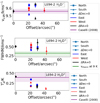 |
Fig. 4 Same as Fig. 3, but for L694-2. |
| In the text | |
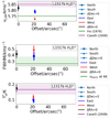 |
Fig. 5 Same as Fig. 3, but for L1517B. |
| In the text | |
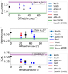 |
Fig. 6 Same as Fig. 3, but for L1544. |
| In the text | |
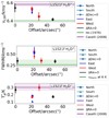 |
Fig. 7 Same as Fig. 3, but for L1521f. |
| In the text | |
|
Fig. 8 Density (solid line) and velocity (dashed line) profiles of a prestellar core predicted by thethree dynamical models: LP flow (green), SIS (red), and QE-BES (blue), as presented in Keto et al. (2015). Each of the modeled profiles was adopted to model the H2D+ emission using RATRAN. |
| In the text | |
|
Fig. 9 Example of the abundance profile adjustment during the fitting process. The observed line profiles of H2D+ are overplotted with the modeled ones using RATRAN toward the central position of the L183 core. Three different dynamical models were adopted, QE-BES, SIS and LP flow. The original abundance profiles (left panel) were adopted by Pagani et al. (2009) and cannot reproduce the central peak of the observations. Adjusting the H2D+ abundance profile by applying a multiplication factor, resulted in a better reproduction of the observations for the LP and QE-BES models, while the SIS model failed to match the shape of the observed line profile. |
| In the text | |
|
Fig. 10 Observed azimuthally averaged line profiles for each position of H2D+ maps toward L183, overplotted with the modeled ones for Static, LP, SIS and QE-BES models from RATRAN. |
| In the text | |
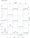 |
Fig. 11 Same as Fig. 10, but for L694-2. |
| In the text | |
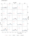 |
Fig. 12 Same as Fig. 10, but for L1517B. |
| In the text | |
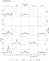 |
Fig. 13 Same as Fig. 10, but for L1544. |
| In the text | |
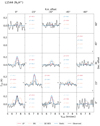 |
Fig. 14 Same as Fig. 10, but for N2H+ toward L1544. |
| In the text | |
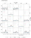 |
Fig. 15 Same as Fig. 10, but for the protostellar core L1521f. |
| In the text | |
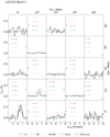 |
Fig. 16 Same as Fig. 10, but for N2H+ toward L1521f. |
| In the text | |
|
Fig. 17 Observed line profiles of H2D+, overplottedwith the modeled ones for LP, SIS, and QE-BES models from RATRAN at selected offsets: (0″, 0″), (15″, 15″), and (−15″, −15″). |
| In the text | |
|
Fig. B.1 Observed line profiles before azimuthal averaging for each position of H2D+ maps toward L183, overplotted with the modeled ones for Static, LP, SIS and QE-BES models from RATRAN. |
| In the text | |
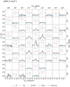 |
Fig. B.2 Same as Fig. B.1, but for L694-2. |
| In the text | |
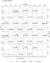 |
Fig. B.3 Same as Fig. B.1, but for L1517B. |
| In the text | |
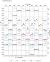 |
Fig. B.4 Same as Fig. B.1, but for L1544. |
| In the text | |
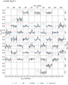 |
Fig. B.5 Same as Fig. B.1, but for N2H+ toward L1544. |
| In the text | |
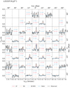 |
Fig. B.6 Same as Fig. B.1, but for L1521f. |
| In the text | |
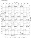 |
Fig. B.7 Same as Fig. B.1, but for N2H+ toward L1521f. |
| In the text | |
Current usage metrics show cumulative count of Article Views (full-text article views including HTML views, PDF and ePub downloads, according to the available data) and Abstracts Views on Vision4Press platform.
Data correspond to usage on the plateform after 2015. The current usage metrics is available 48-96 hours after online publication and is updated daily on week days.
Initial download of the metrics may take a while.