| Issue |
A&A
Volume 643, November 2020
|
|
|---|---|---|
| Article Number | A70 | |
| Number of page(s) | 17 | |
| Section | Cosmology (including clusters of galaxies) | |
| DOI | https://doi.org/10.1051/0004-6361/202038313 | |
| Published online | 05 November 2020 | |
Euclid: The importance of galaxy clustering and weak lensing cross-correlations within the photometric Euclid survey⋆
1
Institute of Space Sciences (ICE, CSIC), Campus UAB, Carrer de Can Magrans, s/n, 08193 Barcelona, Spain
e-mail: tutusaus@ice.csic.es
2
Institut de Recherche en Astrophysique et Planétologie (IRAP), Université de Toulouse, CNRS, UPS, CNES, 14 Av. Edouard Belin, 31400 Toulouse, France
3
Institut d’Estudis Espacials de Catalunya (IEEC), 08034 Barcelona, Spain
4
Instituto de Física Téorica UAM-CSIC, Campus de Cantoblanco, 28049 Madrid, Spain
5
INFN-Sezione di Roma, Piazzale Aldo Moro, 2 – c/o Dipartimento di Fisica, Edificio G. Marconi, 00185 Roma, Italy
6
INAF-Osservatorio Astronomico di Roma, Via Frascati 33, 00078 Monteporzio Catone, Italy
7
INFN-Sezione di Torino, Via P. Giuria 1, 10125 Torino, Italy
8
Dipartimento di Fisica, Universitá degli Studi di Torino, Via P. Giuria 1, 10125 Torino, Italy
9
INAF-Osservatorio Astrofisico di Torino, Via Osservatorio 20, 10025 Pino Torinese, TO, Italy
10
AIM, CEA, CNRS, Université Paris-Saclay, Université Paris Diderot, Sorbonne Paris Cité, 91191 Gif-sur-Yvette, France
11
Institut d’Astrophysique de Paris, 98bis Boulevard Arago, 75014 Paris, France
12
Centre National d’Etudes Spatiales, Toulouse, France
13
Institut d’Astrophysique Spatiale, Universite Paris-Sud, Batiment 121, 91405 Orsay, France
14
Université St Joseph, UR EGFEM, Faculty of Sciences, Beirut, Lebanon
15
Université PSL, Observatoire de Paris, Sorbonne Université, CNRS, LERMA, 75014 Paris, France
16
CEICO, Institute of Physics of the Czech Academy of Sciences, Na Slovance 2, Praha 8, Czech Republic
17
Université de Genève, Département de Physique Théorique and Centre for Astroparticle Physics, 24 Quai Ernest-Ansermet, 1211 Genève 4, Switzerland
18
INAF-IASF Milano, Via Alfonso Corti 12, 20133 Milano, Italy
19
Mullard Space Science Laboratory, University College London, Holmbury St Mary, Dorking, Surrey RH5 6NT, UK
20
Jet Propulsion Laboratory, California Institute of Technology, 4800 Oak Grove Drive, Pasadena, CA 91109, USA
21
CEA Saclay, DFR/IRFU, Service d’Astrophysique, Bat. 709, 91191 Gif-sur-Yvette, France
22
Departamento de Física, FCFM, Universidad de Chile, Blanco Encalada, 2008 Santiago, Chile
23
Astrophysics Research Institute, Liverpool John Moores University, 146 Brownlow Hill, Liverpool L3 5RF, UK
24
INAF-Osservatorio di Astrofisica e Scienza dello Spazio di Bologna, Via Piero Gobetti 93/3, 40129 Bologna, Italy
25
Universitäts-Sternwarte München, Fakultät für Physik, Ludwig-Maximilians-Universität München, Scheinerstrasse 1, 81679 München, Germany
26
Max Planck Institute for Extraterrestrial Physics, Giessenbachstr. 1, 85748 Garching, Germany
27
APC, AstroParticule et Cosmologie, Université Paris Diderot, CNRS/IN2P3, CEA/lrfu, Observatoire de Paris, Sorbonne Paris Cité, 10 Rue Alice Domon et Léonie Duquet, 75205 Paris Cedex 13, France
28
INAF-Osservatorio Astronomico di Capodimonte, Via Moiariello 16, 80131 Napoli, Italy
29
Institut de Física d’Altes Energies (IFAE), The Barcelona Institute of Science and Technology, Campus UAB, 08193 Bellaterra, Barcelona, Spain
30
Department of Physics “E. Pancini”, University Federico II, Via Cinthia 6, 80126 Napoli, Italy
31
INFN Section of Naples, Via Cinthia 6, 80126 Napoli, Italy
32
Institute for Astronomy, University of Edinburgh, Royal Observatory, Blackford Hill, Edinburgh EH9 3HJ, UK
33
European Space Agency/ESRIN, Largo Galileo Galilei 1, 00044 Frascati, Roma, Italy
34
ESAC/ESA, Camino Bajo del Castillo, s/n, Urb. Villafranca del Castillo, 28692 Villanueva de la Cañada, Madrid, Spain
35
Aix-Marseille Univ, CNRS, CNES, LAM, Marseille, France
36
Institut de Ciencies de l’Espai (IEEC-CSIC), Campus UAB, Carrer de Can Magrans, s/n Cerdanyola del Vallés, 08193 Barcelona, Spain
37
Department of Astronomy, University of Geneva, Ch. d’Écogia 16, 1290 Versoix, Switzerland
38
INFN-Padova, Via Marzolo 8, 35131 Padova, Italy
39
Department of Physics & Astronomy, University of Sussex, Brighton BN1 9QH, UK
40
INAF-Osservatorio Astronomico di Trieste, Via G. B. Tiepolo 11, 34131 Trieste, Italy
41
Dipartimento di Fisica “Aldo Pontremoli”, Universitá degli Studi di Milano, Via Celoria 16, 20133 Milano, Italy
42
INFN-Sezione di Milano, Via Celoria 16, 20133 Milano, Italy
43
INAF-Osservatorio Astronomico di Brera, Via Brera 28, 20122 Milano, Italy
44
Leiden Observatory, Leiden University, Niels Bohrweg 2, 2333 CA Leiden, The Netherlands
45
von Hoerner & Sulger GmbH, SchloßPlatz 8, 68723 Schwetzingen, Germany
46
Max-Planck-Institut für Astronomie, Königstuhl 17, 69117 Heidelberg, Germany
47
Aix-Marseille Univ, CNRS/IN2P3, CPPM, Marseille, France
48
Institut de Physique Nucléaire de Lyon, 4, Rue Enrico Fermi, 69622 Villeurbanne Cedex, France
49
European Space Agency/ESTEC, Keplerlaan 1, 2201 AZ Noordwijk, The Netherlands
50
Institute of Theoretical Astrophysics, University of Oslo, PO Box 1029, Blindern, 0315 Oslo, Norway
51
NOVA Optical Infrared Instrumentation Group at ASTRON, Oude Hoogeveensedijk 4, 7991 PD Dwingeloo, The Netherlands
52
Argelander-Institut für Astronomie, Universität Bonn, Auf dem Hügel 71, 53121 Bonn, Germany
53
Institute for Computational Cosmology, Department of Physics, Durham University, South Road, Durham DH1 3LE, UK
54
Université de Paris, 75013 Paris, France
55
LERMA, Observatoire de Paris, PSL Research University, CNRS, Sorbonne Université, 75014 Paris, France
56
Observatoire de Sauverny, Ecole Polytechnique Fédérale de Lau- sanne, 1290 Versoix, Switzerland
57
Dipartimento di Fisica e Astronomia, Universitá di Bologna, Via Gobetti 93/2, 40129 Bologna, Italy
58
INFN-Bologna, Via Irnerio 46, 40126 Bologna, Italy
59
Perimeter Institute for Theoretical Physics, Waterloo, Ontario N2L 2Y5, Canada
60
Department of Physics and Astronomy, University of Waterloo, Waterloo, Ontario N2L 3G1, Canada
61
Centre for Astrophysics, University of Waterloo, Waterloo, Ontario N2L 3G1, Canada
62
Dipartimento di Fisica e Astronomia “G.Galilei”, Universitá di Padova, Via Marzolo 8, 35131 Padova, Italy
63
INFN-Sezione di Bologna, Viale Berti Pichat 6/2, 40127 Bologna, Italy
64
Instituto de Astrofísica e Ciências do Espaço, Faculdade de Ciências, Universidade de Lisboa, Tapada da Ajuda, 1349-018 Lisboa, Portugal
65
Departamento de Física, Faculdade de Ciências, Universidade de Lisboa, Edifício C8, Campo Grande, 1749-016 Lisboa, Portugal
66
Universidad Politécnica de Cartagena, Departamento de Electrónica y Tecnología de Computadoras, 30202 Cartagena, Spain
67
Infrared Processing and Analysis Center, California Institute of Technology, Pasadena, CA 91125, USA
Received:
30
April
2020
Accepted:
8
September
2020
Context. The data from the Euclid mission will enable the measurement of the angular positions and weak lensing shapes of over a billion galaxies, with their photometric redshifts obtained together with ground-based observations. This large dataset, with well-controlled systematic effects, will allow for cosmological analyses using the angular clustering of galaxies (GCph) and cosmic shear (WL). For Euclid, these two cosmological probes will not be independent because they will probe the same volume of the Universe. The cross-correlation (XC) between these probes can tighten constraints and is therefore important to quantify their impact for Euclid.
Aims. In this study, we therefore extend the recently published Euclid forecasts by carefully quantifying the impact of XC not only on the final parameter constraints for different cosmological models, but also on the nuisance parameters. In particular, we aim to decipher the amount of additional information that XC can provide for parameters encoding systematic effects, such as galaxy bias, intrinsic alignments (IAs), and knowledge of the redshift distributions.
Methods. We follow the Fisher matrix formalism and make use of previously validated codes. We also investigate a different galaxy bias model, which was obtained from the Flagship simulation, and additional photometric-redshift uncertainties; we also elucidate the impact of including the XC terms on constraining these latter.
Results. Starting with a baseline model, we show that the XC terms reduce the uncertainties on galaxy bias by ∼17% and the uncertainties on IA by a factor of about four. The XC terms also help in constraining the γ parameter for minimal modified gravity models. Concerning galaxy bias, we observe that the role of the XC terms on the final parameter constraints is qualitatively the same irrespective of the specific galaxy-bias model used. For IA, we show that the XC terms can help in distinguishing between different models, and that if IA terms are neglected then this can lead to significant biases on the cosmological parameters. Finally, we show that the XC terms can lead to a better determination of the mean of the photometric galaxy distributions.
Conclusions. We find that the XC between GCph and WL within the Euclid survey is necessary to extract the full information content from the data in future analyses. These terms help in better constraining the cosmological model, and also lead to a better understanding of the systematic effects that contaminate these probes. Furthermore, we find that XC significantly helps in constraining the mean of the photometric-redshift distributions, but, at the same time, it requires more precise knowledge of this mean with respect to single probes in order not to degrade the final “figure of merit”.
Key words: gravitational lensing: weak / large-scale structure of Universe / cosmological parameters
© ESO 2020
1. Introduction
To better understand the source of cosmic acceleration and the physics of gravity on cosmological scales, large galaxy surveys rely on two main probes: galaxy positions (including redshifts) and weak lensing shapes. Galaxy clustering probes the fluctuations of the underlying dark matter density and velocity fields using the angular and radial positions of galaxies. This can be used for cosmological constraints as it encodes geometric information such as the baryon acoustic oscillations (BAOs; Eisenstein et al. 2005; Aubourg et al. 2015), growth information from redshift-space distortions (RSDs; Percival & White 2009), and more detailed and model-dependent cosmological information encoded in the full shape of the power spectrum (Sánchez et al. 2006; Reid et al. 2010). Similarly, the statistical properties of large ensembles of galaxy shapes can be used to reveal the tiny signal of distortions in their images due to the gravitational potential wells traversed by photons in their propagation towards us – a weak gravitational lensing signal known as “cosmic shear” (see e.g. Kilbinger 2015, for a recent review). This is sensitive to the total amount of matter in the Universe and to the amplitude of its fluctuations, as well as the physics of the gravitational interaction.
Galaxy clustering and cosmic shear are the main probes of the cosmological community’s scientific program for future Stage-IV experiments (Albrecht et al. 2006). In this article we are interested in forecasting the capability of one such future survey: the upcoming European Space Agency (ESA) satellite Euclid (Laureijs et al. 2011), whose characteristics are summarised in Sect. 2. To extract the full information content from Euclid, several systematic effects will have to be taken into account. Some of the more important systematic effects that may affect the cosmological analysis are: the modelling of galaxy bias and redshift-space distortions, photometric-redshift uncertainties and biases, and galaxy intrinsic alignments (IAs; Joachimi et al. 2015).
Here we focus on quantifying the additional information that can be obtained through the cross-correlation (XC) of the angular power spectra of the weak lensing cosmic shear (WL) and galaxy clustering from the photometric sample (GCph) in Euclid. In a previous study (Euclid Collaboration 2020a, hereafter EC20a), it was shown that the combination of the information from WL, GCph, and their XC can result in a significant enhancement of the forecast figure of merit (FoM) on dark energy. The importance of combining WL and GCph to test cosmological models and modified gravity was also previously highlighted by several authors (e.g. Zhang et al. 2007; Song & Percival 2009; Guzik et al. 2010; Reyes et al. 2010; Gaztañaga et al. 2012; Eriksen & Gaztañaga 2015a,b,c, 2018; Fonseca et al. 2015; Blake et al. 2016). Furthermore, as shown by Camera et al. (2017) and Harrison et al. (2016), the XC terms can greatly improve our understanding of systematic effects.
It is important to note that beyond the complementarity between GCph and WL data, GCs measurements are particularly useful when constraining cosmological models, as was shown in EC20a, thanks to the added sensitivity to RSD. Moreover, adding GCs data into the analysis can significantly improve the estimation of the redshift distributions through the clustering-redshift technique (van den Busch et al. 2020).
Other collaborations which have now released their first cosmological results from recent data, such as DES (Troxel et al. 2018; Abbott et al. 2018), KiDS+GAMA (Hildebrandt 2017; Joudaki et al. 2018; van Uitert et al. 2018), and the Hyper-Suprime-Cam (HSC; Hamana et al. 2020; Speagle et al. 2019), also used the power of the joint analysis to improve their constraints. For instance, the DES Collaboration uses the auto- and cross-correlations of two galaxy catalogues. The first catalogue contains the positions of the lens galaxies used for galaxy–galaxy lensing and GCph measurements, while the second catalogue contains the positions and shape measurements of the galaxies used in the WL analysis, which also serve as source galaxies for galaxy–galaxy lensing. The DES Collaboration (see details of the modelling in Krause et al. 2017) works with a data vector that contains the different two-point correlation functions in real space, which in the flat-sky approximation are spherical Bessel integrals over the angular power spectra used in EC20a. Since there are three two-point correlation functions (one for GCph, one for WL, and one for galaxy–galaxy lensing), this joint analysis is also known in the cosmological community as a 3 × 2 pt analysis. This kind of analysis can even be extended by including information from the cosmic microwave background, which leads to a 6 × 2 pt analysis (see e.g. Abbott et al. 2019). On the other hand, the KiDS+GAMA Collaboration uses estimators for the angular power spectra, which they claim to be cleaner in terms of separation of scales (ℓ-modes) than their real-space counterparts (van Uitert et al. 2018). Also, they allow for a separation of the lensing B-modes, which due to their vanishing property can be used as a consistency check. These estimators contain many terms that depend on the survey geometry and data systematic effects, while the angular power spectra used in this work are simplified neglecting many of these survey-specific terms. Apart from that, the differences from our approach lie mostly in the treatment of galaxy bias terms and the intrinsic alignment modelling.
Our goal in this work is to extend the analysis presented in EC20a and assess the impact of including the XC terms when constraining additional cosmological models, and on our understanding of systematic effects. In practice, we consider several different prescriptions for the galaxy bias, photometric-redshift uncertainties, and IAs so that we can determine whether or not the impact of the XC terms on cosmological parameter inference depends on the models used.
After briefly reviewing the Euclid survey in Sect. 2, we present our two probes of choice (the WL and GCph angular power spectra) and the approach we adopt to forecast parameter constraints in Sect. 3. We then present the cosmological model in Sect. 4, and systematic effects in Sect. 5. Finally, we present our results in Sect. 6 and our conclusions in Sect. 7.
2. The Euclid survey
Euclid is an ESA M-class space mission due for launch in 2022, whose near-infrared spectrophotometric instrument (Costille et al. 2018) and visible imager (Cropper et al. 2018) will carry out a spectroscopic and photometric galaxy survey over an area Asurvey = 15 000 deg2 of the extra-galactic sky (Laureijs et al. 2011). The main aims of Euclid are to measure the geometry of the Universe and the growth of structures up to redshift z ∼ 2 and beyond.
In this paper, we focus on the photometric observations that will be used for both a weak gravitational lensing and a galaxy clustering survey. Given the relatively large redshift uncertainties associated with the photometric data –compared to spectroscopy– the analysis of the aforementioned observables will be performed via a so-called tomographic approach. This consists of binning galaxies according to their colour (Kitching et al. 2019) or photometric redshift, which results in tomographic bins that are treated as two-dimensional (projected) data sets. A spherical harmonic decomposition can be performed on the tomographically binned data to create angular (i.e. spherical harmonic) power spectra. In contrast, the accuracy of Euclid’s spectroscopy will allow us to perform galaxy clustering analyses for the spectroscopic sample in three dimensions. It is important to mention that Euclid’s spectroscopy will target objects at high redshift (0.9 < z < 1.8, EC20a), while photometric observations will start at much lower redshift. This motivates the consideration of the complementary information brought by photometric galaxy clustering. The Euclid cosmological probes are therefore three: WL, GCph, and spectroscopic galaxy clustering (GCs).
The XC between WL and GCph is of particular interest because they probe the same observed volume. In this work we focus on this particular XCs, whilst a proper treatment of the XCs between GCph and GCs and between GCs and the WL measurements are left for future work. The modelling of WL and GCph and the recipe used to compute the forecasts for Euclid are described in the following section.
3. Building forecasts for Euclid
In this work we follow for the most part the forecasting recipe presented in great detail in EC20a. We adopt the same Fisher matrix formalism for the computation of the forecasts, as well as the forecasting codes validated therein. However, here we include some important updates, which primarily concern systematic effects such as the implementation of a more realistic galaxy bias model and the inclusion of additional uncertainties on the mean redshift of the tomographic bins caused by potential errors in the photometric redshift determination. These modifications are described in detail in Sects. 5.1 and 5.3 respectively.
For the redshift distribution of galaxies we use the same setup as in EC20a. Galaxies are divided into Nz = 10 tomographic bins as a function of redshift; each bin is equi-populated (i.e. contains the same total number of galaxies) with respect to the true (spectroscopic) redshift:
![$$ \begin{aligned} n^\mathrm{true} (z) \propto \left(\frac{z}{z_0}\right)^2\,{\exp }\left[-\left(\frac{z}{z_0}\right)^{3/2}\right], \end{aligned} $$](/articles/aa/full_html/2020/11/aa38313-20/aa38313-20-eq1.gif)
where  and the surface density of galaxies is
  galaxies per arcmin2. The true (spectroscopic) redshift distribution is then convolved with a sum of two Gaussian distributions (see Eq. (115) in EC20a), in order to provide the observed galaxy distributions in each tomographic photo-z bin, accounting for photometric-redshift errors and the fraction of outliers.
Our observables are the tomographically binned projected angular power spectrum, Cij(ℓ), where ℓ is the angular multipole, and i, j labels redshift pairs of tomographic bins. This formalism is the same for WL, GCph, and the XC terms, with the three cases differing only by the kernels used in the projection from the power spectrum of matter perturbations, Pδδ, to the spherical harmonic-space observable, as detailed in EC20a. Under the Limber, flat-sky, and spatially flat approximations (Kitching et al. 2017; Kilbinger et al. 2017; Taylor et al. 2018), these projections can be expressed as
![$$ \begin{aligned} C^{AB}_{ij}(\ell ) = c\int \mathrm{d}z\,\frac{W^{A}_i(z)W^{B}_j(z)}{H(z)r^2(z)}P_{\delta \delta }\left[\frac{\ell +1/2}{r(z)},z\right], \end{aligned} $$](/articles/aa/full_html/2020/11/aa38313-20/aa38313-20-eq4.gif)
where A and B stand for WL and GCph, r denotes the comoving distance, and H the Hubble parameter. We also ignore reduced shear and magnification effects (Deshpande et al. 2020).
The WL power spectrum contains contributions from cosmic shear and intrinsic galaxy alignments. We assume the latter is caused by a change in galaxy ellipticity, which is linear in the density field. Within this framework, the density-intrinsic and intrinsic-intrinsic 3D power spectra, PδI and PII, respectively, are defined. These depend linearly on the density power spectrum Pδδ, with PδI = −A(z)Pδδ, and PII = [ − A(z)]2Pδδ. For the redshift-dependent amplitude parameter A(z), we use the model specified in Sect. 5.2.
One of the primary sources of uncertainty for galaxy clustering is galaxy bias, that is, the relation between the galaxy distribution and the underlying total matter distribution. Our bias models are discussed in Sect. 5.1.
We use the same redshift bins and number density for both WL and GCph analyses. In practice, this is an over-simplification, because lensing and clustering will apply different probe-specific selection criteria and cuts resulting in different samples. However, for the present Fisher-matrix analysis, we limit ourselves to the same sample for both probes.
In the following we use two different combinations of this observable: WL+GCph where we consider the two to be completely independent and we simply sum the respective Fisher matrices, and WL+GCph+XC. In the latter case, we include the XC terms, that is, we consider the full Gaussian covariance matrix, accounting for all correlations between angular scales, redshift combinations, and correlations between the different observables, thus also including the cross-covariance:
![$$ \begin{aligned}&\mathrm{Cov}\left[C_{ij}^{AB}(\ell ),C_{kl}^{A^{\prime }B^{\prime }}(\ell ^{\prime })\right]\nonumber \\&\qquad \quad =\frac{\delta _{\ell \ell ^\prime }^\mathrm{K}}{(2\ell +1)f_{\rm sky}\Delta \ell }\left\{ \left[C_{ik}^{AA^{\prime }}(\ell )+N_{ik}^{AA^{\prime }}(\ell )\right]\left[C_{jl}^{BB^{\prime }}(\ell ^{\prime })+N_{jl}^{BB^{\prime }}(\ell ^{\prime })\right]\right.\nonumber \\&\qquad \qquad +\left.\left[C_{il}^{AB^{\prime }}(\ell )+N_{il}^{AB^{\prime }}(\ell )\right]\left[C_{jk}^{BA^{\prime }}(\ell ^{\prime })+N_{jk}^{BA^{\prime }}(\ell ^{\prime })\right]\right\} , \end{aligned} $$](/articles/aa/full_html/2020/11/aa38313-20/aa38313-20-eq5.gif)
where A, B, A′,B′ stand for WL and GCph, i, j, k, l run over all tomographic bins,  denotes the Kronecker delta of ℓ and ℓ′, fsky represents the fraction of the sky observed by Euclid, and Δℓ the width of the multipole bins. The noise terms
  take the form
  for WL, where the variance of observed ellipticities is
  , and
, and  for GCph. We assume that the Poisson errors on WL and GCph are uncorrelated, which yields a vanishing noise for XC. More details are laid out in EC20a.
Throughout this study we consider two possible scenarios: an optimistic case and a pessimistic one. Following EC20a, where multipole cuts were introduced to mimic non-Gaussian contribution to the covariances, we define the optimistic case as the analysis where these effects are neglected, including all multipoles from ℓ = 10 to ℓ = 5000 for WL and the multipoles from ℓ = 10 to ℓ = 3000 for GCph and XC. In the pessimistic case, we limit the maximum multipole to 1500 for WL and 750 for GCph and XC, where the limiting multipoles are those for which we reach the maximum information content that one would obtain by including these non-Gaussian contributions.
It is important to mention that a joint analysis of several probes implies a large data vector, which requires a large covariance matrix. In this work we follow EC20a in using a theoretical Gaussian covariance matrix for the observables, which simplifies the estimation of the covariance matrix. However, we must be aware that estimating the joint covariance for analyses with real measurements may become much more difficult than for single-probe analyses; in particular when the covariance is estimated from simulations. In these cases we must ensure that the constraining power brought by the different elements of the data vector is large enough to compensate for the added difficulty on the estimation of the covariance. A simple approach that could be followed is to use only the galaxies that provide the highest signal-to-noise for each probe, that is, use only the sources located at high redshift for WL and the lenses located at low redshift (better photometric redshift estimates) for GCph. Such selection could significantly reduce the dimensionality of the data vector and the covariance and still keep nearly the same constraining power. This was the approach used by Abbott et al. (2018). In this work we want to study the maximum impact of the XC terms. Therefore, we consider the best-case scenario where we can include all the information from all probes without considering the additional difficulty in estimating the covariance matrix. A detailed analysis will need to be done in the future to determine which fraction of the information from each probe can enter into the data vector in order to still be able to accurately estimate the covariance matrix, or to devise data-compression techniques which would allow us to use the full information. However, such analysis is beyond the scope of this work.
4. Cosmological models
We investigate the impact of the XC terms using the cosmological models discussed in EC20a. As baseline, we consider a spatially flat Universe filled with cold dark matter and dark energy. We approximate the dark energy equation of state parameter following the popular parameterisation (Chevallier & Polarski 2001; Linder 2005)
In addition to the two dark energy parameters, w0 and wa, the cosmological model is fully described at the background level by the total matter density at present time, Ωm, 0, and the dimensionless Hubble constant, h, for which we have H0 = 100 h km s−1 Mpc−1; where our notation is that if no time-dependence is specified for a given parameter, we consider this parameter as computed at z = 0.
In addition, the parameters needed to describe the regime of linear perturbations are: the baryon density, Ωb, 0; the slope of the primordial spectrum, ns; and the rms of matter fluctuations on spheres of 8 h−1 Mpc radius, σ8. Concerning the impact of dark energy on matter perturbations, we consider a dynamically evolving, minimally coupled scalar field called Quintessence, where we assume its sound speed is equal to the speed of light, and that it has vanishing anisotropic stress. This implies that we can neglect any fluctuations in the dark energy fluid in our analysis. For the description of linear perturbations we adopt here the parameterised post-Friedmann (PPF) framework of Hu & Sawicki (2007), which allows the equation-of-state parameter to cross w(z) = − 1 without developing instabilities in the perturbation sector.
In addition to this baseline cosmological model, we also explore two extensions, as done in EC20a:
– non-flat models, where the curvature parameter ΩK, 0 is non-zero. In this case we relax the flatness assumption and add the dark energy density ΩDE, 0 as an additional free parameter;
– a modified gravity model with deviations in the standard growth with respect to ΛCDM. We parameterise the growth rate f(z) of linear density perturbations in terms of the growth index γ (Lahav et al. 1991), defined as

with  . The growth rate f is the solution of the equation
![$$ \begin{aligned} f^{\prime }(z)-\frac{f^2(z)}{1+z}-\left[\frac{2}{1+z}-\frac{H^{\prime }(z)}{H(z)}\right]f(z)+\frac{3}{2}\frac{\Omega _{\rm m}(z)}{1+z}=0, \end{aligned} $$](/articles/aa/full_html/2020/11/aa38313-20/aa38313-20-eq14.gif)
where prime refers to the derivative with respect to z, and in general relativity we have γ ≈ 0.55.
Such a modification was implemented in EC20a via a rescaling of the power spectrum P(k, z) in the following way:
![$$ \begin{aligned} P^\mathrm{MG}(k,z) = P(k,z) \left[\frac{D_{\rm MG}(z;\gamma )}{D(z)}\right]^2, \end{aligned} $$](/articles/aa/full_html/2020/11/aa38313-20/aa38313-20-eq15.gif)
where DMG(z; γ) is the growth factor for modified gravity obtained by integrating Eq. (5) for a given γ, keeping in mind that f(z) ≡ − dlnD(z)/dln(1 + z).
The fiducial values for the cosmological parameters vector p also follow EC20a, with

where the last two parameters are considered only in the extended models discussed above. In addition, we fix the sum of the neutrino masses to ∑mν = 0.06 eV. It is important to note that the linear growth factor depends on both redshift and scale in the presence of massive neutrinos. However, we follow EC20a in neglecting this small effect, given the neutrino masses considered in this analysis, and instead compute the linear growth factor in the massless limit. All fiducial values correspond to the ones provided in Planck Collaboration XIII (2016).
5. Systematic effects
While the link between the primary Euclid probes and cosmology is well defined, we necessarily have to account for known systematic effects that can bias our results if not considered properly. In this section we focus on three systematic effects: the galaxy bias, the intrinsic alignment of galaxies, and the uncertainties in the mean of the photometric galaxy distributions in each tomographic bin1. We model each of these in terms of parameterised functions where the additional parameters are known as “nuisance parameters”. This will allow us to marginalise these effects out of our analysis.
In addition to these three mentioned effects, other sources of systematic uncertainties could be considered, but we do not account for these in this paper. As an example, we neglect magnification (Krause & Hirata 2010; Liu et al. 2014; Zitrin et al. 2015; Garcia-Fernandez et al. 2018) and relativistic effects (Yoo & Zaldarriaga 2014; Bonvin 2014; Adamek et al. 2016; Alam et al. 2017a). We note that relativistic effects become relevant at large scales, especially for GCph. To minimise the impact of neglecting these effects on our results, we exclude the largest scales from our analysis, limiting our photometric probes to ℓ ≥ 10.
It is important to mention that in this work we refer to systematic effects as (astro)physical systematic uncertaintites; that is, we only consider systematic effects originating from physical processes. In order for Euclid to reach its expectations, we will have to overcome many observational systematic effects (e.g. Cropper et al. 2013; Euclid Collaboration 2020b), like the removal of foregrounds or the image processing. One major observational challenge for the Euclid photometric survey will be the use of anisotropic ground-based optical data to obtain the photometric redshift estimates of the galaxies detected by the Euclid imager. However, in this work we focus on the systematic effects with a physical origin, because they are intrinsically linked to the signal, while the analysis of observational systematic effects and how we can minimize their impact is left for future work.
5.1. Bias modelling
Weak lensing observations directly trace the underlying matter distribution δm, but the same does not apply for galaxy clustering. This is because galaxy clustering relies on observations of the light from galaxies, which is only a biased proxy of δm (Kaiser 1987). Therefore, in order to obtain theoretical predictions for galaxy clustering observations, the galaxy distribution δg needs to be related to the matter distribution via a bias function, b. This is in general given by
where we neglect the possible dependence of the bias on the scale k, and we assume a linear relation between the matter and galaxy distributions. We note that a linear bias approximation is sufficiently accurate for large scales (Abbott et al. 2018). However, when adding very small scales into the analysis, or using for instance spectroscopic galaxy clustering, a more detailed modelling of the galaxy bias is required (see e.g. Sánchez et al. 2017). One of the approaches to this modelling is through perturbation theory, which introduces a non-linear and non-local galaxy bias (Lazeyras et al. 2016; Chan et al. 2012; Sheth et al. 2013; Desjacques et al. 2018; see also Pandey et al. 2020; Sugiyama et al. 2020 for galaxy bias modelling with DES and HSC mock catalogues, respectively).
Constraints coming from galaxy clustering alone will be affected by the marginalisation over nuisance parameter constraints used to model b(z), as these will be degenerate with cosmological parameters. However the inclusion of weak lensing information (which does not depend on galaxy bias) and the XC between these two probes breaks these degeneracies and therefore improves the constraints on cosmological parameters, while also providing information on the galaxy bias itself.
In this paper we are interested in quantifying the increase in information stemming from inclusion of the XC terms, and deciphering whether or not the use of this additional information will allow us to improve our knowledge on b(z) within the context of different possible bias models. To achieve this, we investigate the impact of XCs on two different parameterisations of b(z):
– Baseline (binned) bias (EC20a), where the bias is assumed to be constant within each of the redshift bins in true redshift, that is,
with zi and zi + 1 being the boundaries of the ith redshift bin in true redshift.
– Flagship bias, where we use a fitting function in agreement with the measurements obtained from the Flagship simulation of the Euclid survey2:
![$$ \begin{aligned} b(z) = A+\frac{B}{1+\mathrm{exp}\left[-(z-D)C\right]}, \end{aligned} $$](/articles/aa/full_html/2020/11/aa38313-20/aa38313-20-eq19.gif)
where A, B, C, and D are nuisance parameters.
In the first case, we choose a fiducial for our nuisance parameters corresponding to the choice
Therefore, the fiducial values of the nuisance parameters are

with  the mean redshift value of each redshift bin in true redshift.
For the Flagship galaxy bias model we use fiducial parameters measured directly from the simulation, which are: A = 1.0, B = 2.5, C = 2.8, and D = 1.6. These values were obtained by selecting all galaxies from the Flagship simulation with a magnitude in the Euclid VIS band of less than 24.5, which corresponds to the magnitude cut where extended sources will be detected at 10σ in four exposures lasting 565 s each (Cropper et al. 2018). Once the galaxies from the simulation have been selected, we measure their galaxy clustering projected angular power spectra at different redshifts. We then obtain the galaxy bias by computing the ratio of these spectra to the theoretical matter predictions.
It is important to note that in the Flagship case we make the assumption that we will be able to parameterise the redshift evolution of the galaxy bias. In the binned case, on the other hand, we consider several free parameters (one for each redshift bin) without attempting to model the redshift evolution within each bin. Therefore, we are not only considering two different fiducial functions for our galaxy bias evolution, but are also testing the role of XC when our ability to parameterise the redshift evolution of galaxy bias is different.
In Fig. 1 we show the fiducial galaxy bias for both parameterisations. For illustrative purposes we also show the trend in redshift of the binned and Flagship models with respect to their fiducial values when the bias nuisance parameters are varied, with a random Gaussian dispersion of 5%. It is important to mention that the trend of the Flagship galaxy bias beyond z = 2 is caused by the extrapolation of the analytic parameterisation used to fit the measurements to the simulation. However, the number density of galaxies in this region is very low, which implies that the extrapolation used will have a negligible impact on the final results.
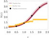 |
Fig. 1. Different bias parameterisations used in the paper: the binned bias (orange line) and the Flagship bias (red line), for the fiducial values of their respective parameters. Also shown are the measurements of the galaxy bias in the Flagship simulation (black dots). For illustrative purposes, a further 25 lines for each case are represented alongside the fiducials, showing how the galaxy bias changes when we allow for a Gaussian dispersion of 5% on the bias nuisance parameters. |
Although our baseline modelling for galaxy bias assumes a linear approximation, we further consider a simple non-linear extension to check the dependence of the XC terms on the linear bias assumption. We follow Baldauf et al. (2010) in assuming a local, non-linear galaxy bias relation via a Taylor expansion of the galaxy density field as a function of the matter overdensity. We note that we are setting the non-local terms (McDonald 2006; McDonald & Roy 2009) to zero for simplicity, but this local non-linear model is adequate for our purposes. We can in this case rewrite Eq. (9) as
where bL stands for the linear galaxy bias and bNL represents its non-linear contribution.
The galaxy–galaxy and galaxy–matter power spectra are then given by


where N is the renormalised shot noise, PNL represents the non-linear matter power spectrum, and PA and PB are given by
![$$ \begin{aligned}&P_{B}(k) =\int \frac{\mathrm{d}^3q}{(2\pi )^3}P_{\rm L}(|\boldsymbol{q}|)[P_{\rm L}(|\boldsymbol{k}-\boldsymbol{q}|)-P_{\rm L}(q)], \end{aligned} $$](/articles/aa/full_html/2020/11/aa38313-20/aa38313-20-eq27.gif)
with PL being the linear matter power spectrum and
being the second-order standard mode coupling kernel. Following Baldauf et al. (2010), we set our bNL fiducial such that the ratio bNL/bL is equal to 0.26. We note that the specific fiducial value does not have a relevant role when trying to determine the role of XC beyond the linear galaxy bias approximation. However, a fixed ratio of bNL/bL = 0.26 is also in agreement with the results obtained in Pandey et al. (2020) for the range of bL baseline values considered in this work. We further set the renormalised shot noise N = 0.
5.2. Intrinsic alignment
In Sect. 3, we defined the IA amplitude parameter A. In our approach, this parameter takes the form given in EC20a:
where 𝒞IA is a normalisation parameter which we set as 𝒞IA = 0.0134, D(z) is the growth factor, and 𝒜IA is a nuisance parameter fixing the overall amplitude of the IA contribution. The function ℱIA sets the redshift dependence of the IA contribution which can be conveniently modelled as
![$$ \begin{aligned} \mathcal{F} _{\rm IA}(z) = (1 + z)^{\eta _{\rm IA}} \left[ \frac{\langle L \rangle (z)}{L_{\star }(z)}\right]^{\beta _{\rm IA}}, \end{aligned} $$](/articles/aa/full_html/2020/11/aa38313-20/aa38313-20-eq30.gif)
with ⟨L⟩(z)/L⋆(z) being the redshift-dependent ratio between the average source luminosity and the characteristic scale of the luminosity function. Equations (20) and (21) reduce to the non-linear alignment model (Hirata et al. 2007; Bridle & King 2007) for ηIA = βIA = 0 (i.e. ℱIA = 1), while the additional scaling with z and the luminosity has been introduced to improve the fit to both low-redshift data and numerical simulations (Joachimi et al. 2015). We refer to this model as eNLA in the following, setting the nuisance parameters to the following fiducial values

in accordance with the recent fit to the IA measured in the Horizon-AGN simulation (Chisari et al. 2015). It is important to mention that we expect the amplitude of IA, 𝒜IA, to be smaller in practice (see Fortuna et al. 2020, for a detailed discussion on the amplitude of IA for different types of galaxies), but we keep a higher value in this analysis to study the role of XCs when IA are important.
5.3. Photometric redshifts
The accuracy of photometric redshifts is crucial to the exploitation of the galaxy clustering and weak lensing power spectra. To mitigate the effect of potential unknown biases in the photo-z algorithms, we follow Troxel et al. (2018) and Abbott et al. (2018) who introduced nuisance parameters for the biases and/or shifts of the mean redshifts of each photo-z bin, that is,
where Δzi is a nuisance parameter for each redshift bin, and  is the true galaxy distribution. This change of the galaxy redshift distribution is going to impact galaxy clustering and weak lensing predictions through their kernels. Δzi > 0 will generally lead to a higher amplitude for clustering and a lower amplitude for weak lensing, as the galaxies are shifted to lower redshifts. Because the XC terms increase the number of spectra used in a likelihood analysis with respect to the number of redshift bins (and thus the number of nuisance parameters), it may be expected that including these terms will improve the constraints on these nuisance parameters. Before moving to the results section we summarise all the nuisance parameters considered in this analysis in Table 1 together with their fiducial values.
Summary of nuisance parameters considered in this analysis together with their fiducial values.
6. Results
In this section, we present the main results of our analysis, namely the improvement in parameter constraints using the Euclid WL and GCph probes when also including their XC terms, instead of simply considering the two probes as independent. The effect of XC on cosmological parameter constraints was briefly discussed in EC20a; here instead we focus in particular on the importance of the XC terms in constraining the nuisance parameters, as they also contain astrophysical information, for example in testing galaxy formation scenarios. In this section, unless otherwise stated, all the plots refer to the “optimistic” case.
6.1. Baseline specifications
Let us start by considering the baseline specifications described above. In this work we follow the definition of FoM used in EC20a:  , with
  being the marginalised Fisher submatrix for w0 and wa. Our baseline specifications are the same as those adopted in EC20a, where the impact of XC terms on cosmological parameter constraints was discussed, finding an improvement in the FoM of a factor 5.7 (4.4) for the pessimistic (optimistic) case when a flat cosmology is assumed, a result that is confirmed by the analysis performed in this work. Here we focus instead on the impact of the XC terms on both the cosmological and nuisance parameters. In the top panel of Fig. 2 we show the ratio on the forecast uncertainties for the bias parameters with and without XC, that is, σ(bi,WL+GCph)/σ(bi,WL+GCph+XC). We also report the marginalised constraints on the ten bias parameters in Table A.1. Comparing the results with and without XC immediately shows the power of this additional information in reducing the error on the bias parameters. On average over the ten parameters, we find an error reduction of ∼9% (∼25%) in the pessimistic (optimistic) scenario when XC is included.
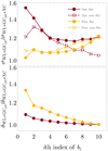 |
Fig. 2. Ratio of the marginalised (top panel) and unmarginalised (bottom panel) forecast uncertainties on the bi bias parameters between WL+GCph and WL+GCph+XC, in the pessimistic (red lines) and optimistic (yellow lines) cases. We show in this plot results for both the flat Universe model (solid lines) and the non-flat case (dashed lines). |
It is interesting to note that there is a qualitative trend of σ(bi,WL+GCph)/σ(bi,WL+GCph+XC) with the bin redshift. In particular, we find that the above ratio increases with z in the pessimistic case (going from 1.09 to 1.21), while the trend is reversed in the optimistic case (the ratio decreasing from 1.54 to 1.20). Moreover, the improvement brought by the XC is significantly larger for the optimistic case than for the pessimistic one. In order to understand these effects, we investigated the ratio of the unmarginalised constraints on the galaxy bias nuisance parameters, instead of marginalising over the cosmological and IA parameters, which is shown in the bottom panel of Fig. 2. In the unmarginalised case we observe that both the optimistic and pessimistic scenarios show a similar trend as a function of redshift. Moreover, the improvement on the constraints given the addition of XCs is larger in the pessimistic case. This is due to the addition of more scales in the optimistic case, which helps in constraining the parameters and therefore slightly decreases the additional constraining power of the XC. Therefore, the different behaviour in the top panel of Fig. 2 is entirely due to the correlations between the cosmological and nuisance parameters.
It is worth investigating whether or not the reduction in error caused by the inclusion of the XC is model independent. To this end, we consider the case of non-flat models, that is, we still leave the fiducial model unchanged, but relax the flatness assumption adding the fractional density of dark energy, ΩDE, 0 as an additional parameter to constrain; we note that we still assume flatness in the Limber approximated power spectra (Taylor et al. 2018). We refer again to Fig. 2 for the ratio of the constraining power with and without XC, while we show the marginalised errors on the bias parameters for both pessimistic and optimistic assumptions in Table A.2. As expected, adding one more parameter weakens the overall constraints due to the increased volume in parameter space and degeneracies among the full set of cosmological and nuisance parameters. This increase in the marginalised errors occurs whether XC is included or not. With respect to the flat case, we find, on average, a 35% increase of the errors for WL+GCph compared to a 32% increase when XC is added in the pessimistic case, while these numbers become 7% and 17% in the optimistic case. When comparing WL+GCph with WL+GCph+XC constraints for non-flat models, we again find that XC reduces the marginalised errors on the bias parameters. We also find the same trend with redsfhit for the impact of XC: larger impact at low redshift and smaller impact at high redshift for the optimistic case, while the impact as a function of redshift increases for the pessmistic case. In the non-flat case we observe a smaller effect than in the flat case for the optimistic assumption with an average improvement due to the addition of XC of 15% instead of 25%. The opposite is true in the pessimistic case, where the average improvement is of 12% instead of 9%. Given the different range in multipoles between the optimistic and pessimistic cases, the degeneracies introduced by the additional parameter ΩDE, 0 are lifted in the optimistic case by the use of small scales, while in the pessimistic case XC plays a more important role, thus increasing its relevance with respect to the flat cosmology.
We now discuss the constraints on the IA parameters for the eNLA model, which we summarise in Table 2 in both the flat and non-flat cases under both pessimistic and optimistic assumptions. We find that the marginalised errors of the IA parameters are of the same order of magnitude as (if not larger than) the fiducial values. However, this is not unexpected when considering that they only enter through their combination in 𝒜IAℱIA(z), meaning that large degeneracies are present in the amplitude terms. Indeed, we find that the correlation coefficient of for example 𝒜IA with (ηIA, βIA) is almost unity. In addition, the GCph probe is totally independent of IAs and therefore does not constrain the IA parameters at all. As a consequence, adding WL and GCph has only an indirect impact on the IA constraints. To understand how this works, let us focus on the correlation between 𝒜IA and Ωm, 0 which is one of the closest correlations in the optimistic case. When using WL alone, we find a correlation coefficient of −0.27 which reduces to −0.12 when using WL+GCph because of the better constraint on Ωm, 0. However, the error on 𝒜IA is not particularly affected by this with σ(𝒜IA) reducing from 3.47 to 3.35, that is, a 4% reduction only. Instead, when XC is included, the degeneracy between Ωm, 0 and 𝒜IA is almost totally lifted with the correlation coefficient going down to −0.007, thus allowing an improvement of almost a factor of 3.5. We show the impact of XC on IA parameter constraints in Fig. 3 for the optimistic case. The inclusion of XC improves the constraints on {𝒜IA, ηIA, βIA}, but the expected errors are smaller than the corresponding fiducial value only in the optimistic scenario. It is also worth noting that relaxing the flatness assumption does not degrade the constraints on the IA parameters. This is just a consequence of the IA parameters being almost uncorrelated with ΩDE, 0 and means that there are no further degeneracies introduced. For this same reason, the impact of XC works in the same way as for the flat case, because the same qualitative argument still holds in the non-flat case.
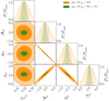 |
Fig. 3. 1σ and 2σ confidence contours on the optimistic, flat GR baseline case for GCph+WL (orange) vs. GCph+WL+XC (green) for the three intrinsic alignment parameters compared to the Ωm, 0 parameter. While the IA parmeters are clearly highly degenerate among themselves, Ωm, 0 shows little degeneracy with them, especially when XC is included. |
Constraint on the IA nuisance parameters for flat and non-flat cases for both the pessimistic and optimistic assumptions.
To conclude this section, which focuses on the specifications and models under investigation in EC20a, extending the investigation to the effects of XC on nuisance parameters, we want to quantify the impact of the XC terms on modified gravity constraints. Here we use the phenomenological approach described in Sect. 4, that is, we consider the growth index γ. In the ΛCDM concordance model, γ ≈ 0.55, with gravity described by general relativity. A deviation from this value could be indicative of phenomena associated with modified gravity. To forecast how accurately Euclid photometric probes can constrain this parameter, we add γ as a new parameter in the Fisher matrix by the simple extension of the general relativity recipe from Sect. 4. In this case, we find a significant weakening of the constraints as a consequence of including this additional parameter, as expected. More interestingly, we also find that XC is highly efficient in improving the constraints on each cosmological parameter compared with WL+GCph only. This is consistent with the findings of EC20a for the general relativity model considered, and we now extend this result to the modified gravity case. In particular, the error on γ reduces by a factor of 1.5 in the pessimistic case showing that XC helps to constrain deviations from general relativity. The impact is less pronounced when one includes larger ℓ, with XC reducing the error in the optimistic case by only 10% which is due to the fact that in the optimistic case the constraints are now driven by the non-linear part of the power spectrum. In this work we model the non-linearities following the same prescriptions of EC20a, which are obtained in the ΛCDM regime. However, an adapted recipe for non-linearities should be applied for each modified gravity theoretical model, which could change the quantitative impact of XC depending on the modified gravity model considered.
We show the effect of XC on γ constraints in Fig. 4. We report the 68% errors on this and the other cosmological parameters in Table A.3, while we show the constraints on the bias parameters in Table A.4.
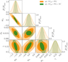 |
Fig. 4. 1σ and 2σ confidence contours on the optimistic, flat, modified gravity baseline case for GCph+WL (orange) vs. GCph+WL+XC (green). The modified gravity parameter γ is not significantly better constrained when including XC, but its inclusion helps to break some degeneracies, especially with w0, wa, and σ8. |
In contrast with the cosmological parameters, the marginalised errors on the IA parameters are not affected by the presence of the γ parameter, and therefore the effect of XC on these is unchanged. This is a consequence of the interplay among the degeneracy of IA and cosmological parameters which is now changed with respect to the general relativity case. As a result, the weakening of the constraints on cosmological parameters does not lead to a corresponding increase in the errors for the IA parameters.
We also investigated the case where the flatness assumption is relaxed, leaving ΩDE, 0 free to vary. We do not find any remarkable difference on the impact of XC, apart from the expected degradation of the constraints due to having one more parameter.
Finally, we re-computed the baseline forecasts including priors on the cosmological parameters coming from the spectroscopic galaxy clustering analysis of Euclid from EC20a and from the final BOSS data release (Alam et al. 2017b); therefore neglecting the XC terms that might appear between GCs and the photometric probes. Both for the baseline flat model and for the non-flat modified gravity case, we see that the effect of XC (on the constraints of both the cosmological and nuisance parameters) is equally significant when we add priors coming from BOSS. When adding priors coming from the GCsEuclid analysis, the effect of the XC terms is slightly weaker, given the significant increase in constraining power by the additional probe. However, the XCs are still a vital addition when constraining the cosmological and nuisance parameters.
6.2. Dependence on the galaxy bias model
Galaxy bias enters both the GCph and XC terms, and therefore it is worth considering how the cosmological constraints depend on the bias model. In the baseline specifications, b(z) was modelled as a piecewise constant function with independent amplitudes in the ten redshift bins. However, N-body simulations coupled with reliable models for galaxy distributions and halo occupation statistics can provide a physically motivated prior on the redshift dependence of the bias function. Using this information, we model b(z) using Eq. (11), with the four parameters {A, B, C, D} as the new nuisance parameters free to vary in our Fisher analysis.
As we reduce the number of nuisance bias parameters from 10 to 4, or in other words we assume we can parameterise the redshift evolution of the galaxy bias even within each redshift bin, we expect an improvement of the constraints on the cosmological parameters. In Table A.5 we report the marginalised errors for the flat general relativity case3 which can be compared with the corresponding table from EC20a. Averaging over the full set of parameters, we indeed find a 17% (14%) reduction of the WL+GCph (WL+GCph+XC) errors for the pessimistic case, which is due to the more rigid bias modelling; this factor reduces to 4% (6%) in the optimistic case. We also find that reducing the number of bias parameters reduces the correlation between parameters, as can be seen when looking at the FoM. The WL+GCph FoM indeed increases by 37% (15%) for the pessimistic (optimistic) case, while the WL+GCph+XC FoM improves by 54% (30%). Although not unexpected, this significant boost of the FoM highlights the importance of constraining the galaxy bias in the GCph sample.
Regardless of the bias model used, adding XC to WL and GCph still stands out as the most efficient way to strengthen the constraints on the cosmological parameters, and also increase the FoM. In detail, the impact of XC for the pessimistic case is large, with FoM(WL + GCph + XC)/FoM(WL + GCph) = 5.7 for the binned bias modelling. This factor reduces somewhat to FoM(WL + GCph + XC)/FoM(WL + GCph) = 4.8 when the Flagship bias modelling is adopted. For the optimistic case, these ratios are 4.4 and 3.7, respectively. This reduction of the impact of XC when moving from binned bias to Flagship bias is related to the Flagship bias already removing part of the degeneracy between cosmological and nuisance quantities thanks to its smaller number of parameters. The numbers are nevertheless still large enough that the impact of XC is of paramount importance.
Let us now discuss the constraints on the bias and IA nuisance parameters reported in Table 3. Concerning the bias parameters, a direct comparison with the baseline case of Table A.1 is not possible as we use different parameterisations. We nevertheless note that the impact of XC on the constraints is comparable to the binned bias case. Indeed, we find that adding XC reduces the errors on average by 8% (27%) in the pessimistic (optimistic) case which is roughly the same as what we found for the binned bias case. Again, this is consistent with expectations, because the effect of XC is to reduce the correlation among the bias and the cosmology, and this happens no matter which bias model is used.
68% errors, without and with the XC contribution, on the nuisance parameters (both bias and IA) when the Flagship bias model is considered.
Moreover, we find that the constraints on the IA nuisance parameters are not modified with respect to the binned bias case. This happens because bias and IA are two different phenomena affecting only GCph and WL, respectively, but not both of them. Therefore, the bias model has no impact on IA constraints and the effect of XC on those is similar to what was found in the baseline case.
In addition, we investigated the effect of the change in the bias modelling on constraints on the modified gravity parameter γ. We find σ(γ) = 0.046 (0.017) for the pessimistic (optimistic) case using only WL+GCph, while adding XC reduces the error to σ(γ) = 0.036 (0.014), which is a 27% (21%) improvement. Cross-correlation has a different impact on γ with respect to the binned bias case, where the improvement was of 50% in the pessimistic case and of 10% in the optimistic one. The different relevance of XC in this case is connected to the significant improvement that a change in the bias modelling brings on σ(γ). Replacing the binned bias with the Flagship one improves the constraints on γ by a factor of ∼1.5 for both the pessimistic and optimistic cases when WL+GCph+XC is used. We can therefore conclude that a reliable modelling of the galaxy bias is of significant value when discriminating general relativity and modified gravity models based on the growth of structures.
Before finishing this section, we study the impact of the XC terms when we go beyond the linear galaxy bias approximation. We consider, for simplicity, the baseline specifications with ten tomographic bins and a constant bL per bin with fiducial  , where
  denotes the mean of the bin in true redshift. We further consider a constant bNL per tomographic bin with fiducial bNL = 0.26bL, as described in Sect. 5.1, which leads to a total of 20 nuisance parameters for the galaxy bias. Looking first at the cosmological parameter constraints, we find that adding the XC terms when using a non-linear galaxy bias model improves the constraints by between a factor of 1.5 and 3.4 for the pessimistic case, and between a factor of 1.3 and 2.5 for the optimistic case (compared to the constraints with a non-linear galaxy bias model and without the XC terms). This improvement should be compared to a factor of between 1 and 3.5 (1.1 and 2.6) for the pessimistic (optimistic) case when using a linear galaxy bias model. Therefore, we can confirm that the additional constraining power on the cosmological parameters from the XC between GCph and WL is still present when we consider a more complex galaxy bias model. Moreover, in the case of a non-linear galaxy bias model, the addition of the XC terms allows us to improve the constraints on bL by a factor of between 1.4 and 2 (1.6 and 2.4) for the pessimistic (optimistic) case. This can be compared to the improvement on the galaxy bias constraints (using the linear model) when adding the XC terms, which corresponds to an improvement by a factor of between 1 and 1.2 (1.2 and 1.5) for the pessimistic (optimistic) case, as shown in Fig. 2. Thus, the XC between GCph and WL is even more helpful when constraining more complex galaxy bias models.
6.3. Shift in cosmological parameter best fit from neglecting IA
In Sect. 5.2 we describe how we include the IA contribution in the theoretical predictions for cosmic shear, while in Sect. 6.1 we estimate the improvement brought by XC on the constraints of the parameters modelling this effect. Given the constraining power brought by GCph and XC in addition to the WL probe, it is worth exploring whether or not such a combination can be used to distinguish different assumptions pertaining to this contribution.
To estimate whether or not one can distinguish between different models of a physical mechanism, the shift in the best fit of the cosmological parameters with the ‘wrong’ model can be tested. In an MCMC (of nested sampling) analysis this could be estimated by generating mock data with a given fiducial cosmology and fitting these with theoretical predictions from a different one; the cosmological parameters will be shifted from the assumed fiducial values in order to compensate the different effects of the two cosmologies.
However, this investigation can also be performed within the Fisher matrix formalism if we deal with “nested models”, where the parameter space of one of the two cosmologies is contained within that of the other (Heavens et al. 2007). In this framework, the former cosmology is described by a set of parameters {θα}, while the latter by {θα}∪{ψa}, and we note that in this treatment we label the nested model parameters by indexes α, β, and so on, and the extra parameters by indexes a, b, and so on. This leads us to question what happens to the best-fit estimates of the parameter set θ if we do not properly model ψ in our analysis. For instance, if reality is described by the parameter  and we wrongly assume
  as the fiducial cosmology, this will imply a shift in the θ parameters due to a compensation that has to account for ψ being kept fixed to an incorrect value. In a Fisher matrix analysis, such a shift δ on a parameter θα can be computed via (see Camera et al. 2017, Appendix A)

where it is worth emphasising that F is the full Fisher matrix containing both parameter sets θ and ψ, whereas Fβa are the elements of the rectangular sub-matrix mixing θ and ψ parameters, and summation over equal indexes is assumed.
We apply such a methodology to investigate whether or not the combination of GCph, WL, and their XC is able to distinguish different amplitudes 𝒜IA of the IA contribution. To this end, we keep the fiducial of βIA and ηIA to our baseline, but we use Eq. (24) to compute the shift on the cosmological parameters caused by an incorrect assumption of 𝒜IA. The results for Ωm, 0, w0, and wa are shown in Fig. 5, where we highlight the significance of this shift when 𝒜IA is changed from the baseline fiducial4. We see that completely neglecting the IA contribution (𝒜IA = 0) leads to shifts of ≈40σ on Ωm, 0, ≈20σ on w0 and ≈10σ on wa when the full combination WL+GCph+XC is considered. If we do not include XC, such shifts reduce to ≈3σ, ≈5σ, and ≈5σ, respectively, which demonstrates how the addition of XC is relevant not only to improve the constraining power of the survey, but also to test the assumptions made in the modelling of nuisance effects. It is important to point out here that the huge values of the shifts on the parameters when XC is included should not be taken literally; when the shift with respect to the fiducial values becomes large, the Gaussian approximation on which the Fisher matrix analysis relies breaks down. Therefore, the Fisher approximation can no longer capture the true shape of the likelihood. We consider the value of 3σ as a safe threshold, meaning that any shift beyond this limit should be interpreted as simply a very large shift. We represent this region in Fig. 5 with a grey-shaded area.
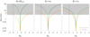 |
Fig. 5. Shifts in units of standard deviations for Ωm, 0 (left panel), w0 (middle panel), and wa (right panel) due to an incorrect assumption on the IA amplitude. Results are shown for the optimistic case with WL+GCph (orange) vs. WL+GCph+XC (green). Solid (dashed) lines represent positive (negative) shifts with respect to the fiducial. The vertical grey line shows the case in which we assume no contribution from IA (𝒜IA = 0). The grey-shaded region denotes the shifts larger than 3σ, for which the Gaussian approximation breaks down and the corresponding shifts should be interpreted with caution (see the text for details). |
It is worth mentioning before concluding this section that we have also considered applying this extended Fisher formalism to quantify the shift in the cosmological parameter best fit from assuming a “wrong” fiducial galaxy bias. In more detail, we first assumed that our galaxy bias could be modelled by a piecewise constant function5. We then used Eq. (24) to compute the shift in cosmological parameters when we consider the fiducial  but the “truth” is given by the Flagship fiducial described in Sect. 5.1. We obtained even larger shifts than for the IA case, which go from 4σ for ns up to very biased (more than 40σ) for w0 and wa when we consider the optimistic WL+GCph+XC case. Since XC partially removes the degeneracy between the cosmological and galaxy bias parameters, the shifts become even larger when XC is not included. It is important to recall that given the large shifts these values should only be interpreted qualitatively, since they are significantly beyond the 3σ safe threshold. These results show that our knowledge on the galaxy bias has a significant impact on the cosmological conclusions derived from the observations.
6.4. Impact of XC on photo-z self-calibration
In the above sections we implicitly assume that photometric redshifts have been measured with perfect average accuracy, that is, that the mean true redshift of a bin is indeed equal to the mean measured redshift. However, as pointed out in Sect. 5.3, we can consider the possibility of an error Δzi systematically shifting the redshift of all the sources in the ith bin. Allowing for an arbitrary deviation, we can include ten additional nuisance parameters Δzi. We can then investigate both how well these quantities must be known so as not to degrade the FoM, and which constraints can be put on them by the XC terms.
To this end, we recomputed the Fisher matrices for the baseline case of general relativity, adding the ten Δzi nuisance parameters and fixing their fiducial values to zero6. We add the same Gaussian prior on each one of these nuisance parameters, and we compute the FoM as a function of the width of the prior. We finally compare the output to the case when all Δzi are considered known (FoMref, equivalent to a Dirac delta prior around the fiducial value).
Figure 6 shows the difference between the FoM and the corresponding reference FoMref as a function of the width of the Gaussian prior added, σPrior. This provides the FoM degradation for different combinations of cosmological probes both in the optimistic and pessimistic scenarios. We find that a strong prior is needed if one does not want to degrade the FoM by a large amount. Let us first consider the optimistic case. Starting with the full combination of WL+GCph+XC, we require a prior on the mean of the photometric galaxy distributions smaller than 0.43 × 10⁻³ so as not to degrade the final FoM of 1034 by more than 20%. This threshold is represented in Fig. 6 with a black dot. We note that the prior requirement coming from the other probes may be more stringent if we require a degradation smaller than 20% with respect to the corresponding reference FoM; for instance, we need a prior smaller than 0.31 × 10⁻³ for the WL+GCph combination if we consider the reference WL+GCph FoM, while we only need a prior smaller than 1.60 × 10⁻³ for WL alone (we note that this value is similar to the one provided in Kitching et al. 2008, and the small discrepancies might be due to the different IA modelling and forecasting recipe). However, the combination driving the requirement on the prior is the full combination of WL+GCph+XC, because it is the one providing the highest FoM.
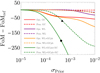 |
Fig. 6. Difference between the FoM and the reference one obtained in the case where all shifts in the mean of the photometric-redshift distributions are perfectly known and equal to zero (Δzi = σ(Δzi) = 0), for a changing value of the prior added. The results refer to GCph (red), WL (purple), WL+GCph (orange), and WL+GCph+XC (green), under pessimistic (dashed) and optimistic (solid) assumptions. The black dot denotes the prior threshold for which the final FoM of the full WL+GCph+XC combination in the optimistic case is degraded by 20%. The black triangle represents the same threshold in the pessimistic case (see the text for details). We note that the reference FoM is larger for the optimistic case in comparison to the pessimistic case, and it increases when the XC terms are included. However, the different lines are normalised to their corresponding reference FoMs for illustrative purposes. |
Focussing now on the pessimistic case, we require a prior smaller than 0.48 × 10⁻³ so as not to degrade the final WL+GCph+XC FoM of 367 by more than 20%. This threshold is represented by a black triangle in Fig. 6.
It is also important to compare the degradation of the FoM as a function of the prior for the different combinations of probes. We can see in Fig. 6 that for the optimistic case the degradation appears earlier (we need a smaller prior) in the full combination of WL+GCph+XC than in the combination WL+GCph. In turn, WL+GCph degrades earlier than GCph alone, which degrades earlier than WL. This is consistent with the values of the FoM for the different combinations of probes, as GCph provides a larger FoM than WL alone, and WL+GCph provides a larger FoM than GCph but smaller than the full combination. Concerning the pessimistic case, we can now observe that we need a more stringent prior for WL than for GCph, which is consistent with the fact that in the pessimistic case the FoM of WL is much larger than the FoM of GCph.
Although reducing Δzi will be achieved by improving photometric redshifts, or by including the clustering-redshift information brought by overlapping spectroscopic surveys of Euclid (see Gatti et al. 2018, for a detailed analysis on how clustering information could help in better determining Δzi), it is nevertheless worth investigating whether or not one can use the data themselves to self-calibrate or constrain Δzi. From this point of view, it is interesting to look at how the constraints change when XC is added to WL+GCph. The result is shown in Fig. 7 for both pessimistic and optimistic scenarios. In this case, XC is indeed of great help in reducing the error on Δzi by a factor 2.2−3.1 as a consequence of both the increased number of observables and the information carried by the correlation among different bins. It is worth noting that the improvement of constraints due to XC is smaller for the optimistic scenario. This is due to the information brought by the additional multipoles included with respect to the pessimistic case, which already add information to constrain these nuisance parameters and reduce the impact of XC.
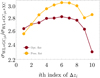 |
Fig. 7. Ratio of the errors on Δzi with and without the inclusion of XC. Yellow and red lines refer to the pessimistic and optimistic scenario. |
7. Conclusions
In this paper, we extensively scrutinise the impact on both cosmological and nuisance parameter estimation of the cross-correlations (XC) between two probes of the Euclid satellite mission: weak lensing cosmic shear (WL) and the clustering of the photometric galaxy sample (GCph).
Let us first emphasise that the XC terms must necessarily be included in the data vector because both WL and GCph trace the same underlying cosmic structure and are therefore not independent from one another. This implies that a failure to include the XC terms will lead to an incorrect estimation of the constraining power, with associated consequences for model testing. The scope of this paper is to assess the impact of such XC.
In EC20a it was demonstrated that rather than being a nuisance, XC encodes valuable cosmological information. In that paper, we found that the best cosmological constraints are obtained when XC is taken into account, leading to an increase of the FoM by more than a factor of three for a flat Universe. Here we focus on showing that XC is crucial also to constrain nuisance parameters.
Our main findings can be summarised as follows:
-
On average, the uncertainty on the galaxy bias amplitude nuisance parameters is reduced by ∼9% and ∼25% when XC is included, for the pessimistic and optimistic scenario, respectively.
-
The inclusion of XC makes IA parameters detectable (in the optimistic scenario), and this result is not affected by the assumptions of flatness and the validity of general relativity.
-
A different bias model does not directly impact the effect of XC on cosmological and nuisance parameters. However, the lower number of parameters needed to describe the galaxy bias significantly affects the constraints on deviations from general relativistic growth of structures, parameterised by γ. This in turns also changes the impact of XC on this same parameter.
-
Given the tighter constraints allowed by XC, the interplay between different parameters becomes more important, and incorrect assumptions on systematic-effect parameters such as IA may lead to significant degradation of the survey accuracy in cosmological parameter estimation.
-
The addition of XC significantly helps in constraining the mean of the photometric-redshift distributions. However, the requirement on the knowledge of the mean is much more stringent than for WL alone in order not to degrade the final FoM.
We can conclude that the addition of XC between cosmic shear and galaxy clustering for the photometric Euclid survey is necessary for the analyses of the future data. Not only do XCs improve our knowledge of the cosmological model, but they also provide information about galaxy bias, IAs, and help in self-calibrating the photometric galaxy distributions.
We note that the extended Fisher formalism used in this work can only accommodate nested models. Because of this we cannot compute the shift when changing the fiducial and the parameterisation of the galaxy bias at the same time, as is done in Sect. 5.1.
Acknowledgments
This work started in the cross-correlation group, led by A. Blanchard, M. Kunz, and F. Lacasa, of the Inter-Science Working Group Task-force for forecasting of the Euclid Consortium. I. Tutusaus acknowledges support from the Spanish Ministry of Science, Innovation and Universities through grant ESP2017-89838-C3-1-R, and the H2020 programme of the European Commission through grant 776247. M. Martinelli has received the support of a fellowship from “la Caixa” Foundation (ID 100010434), with fellowship code LCF/BQ/PI19/11690015, and the support of the Spanish Agencia Estatal de Investigacion through the grant “IFT Centro de Excelencia Severo Ochoa SEV-2016-0597”. S. Camera acknowledges support from the “Departments of Excellence 2018−2022” Grant awarded by the Italian Ministry of Education, University and Research (MIUR) L. 232/2016. S. Camera is supported by MIUR through Rita Levi Montalcini project “PROMETHEUS – Probing and Relating Observables with Multi-wavelength Experiments To Help Enlightening the Universe’s Structure”. F. Lacasa acknowledges support by the Swiss National Science Foundation. S. Ilić acknowledges financial support from the European Research Council under the European Union’s Seventh Framework Programme (FP7/2007–2013)/ERC Grant Agreement No. 617656 “Theories and Models of the Dark Sector: Dark Matter, Dark Energy and Gravity”. V. Yankelevich acknowledges funding from the European Research Council (ERC) under the European Union’s Horizon 2020 research and innovation programme (grant agreement No. 769130). P. Ntelis is funded by “Centre National d’Études Spatiales” (CNES), for the Euclid project. The Euclid Consortium acknowledges the European Space Agency and the support of a number of agencies and institutes that have supported the development of Euclid, in particular the Academy of Finland, the Agenzia Spaziale Italiana, the Belgian Science Policy, the Canadian Euclid Consortium, the Centre National d’Etudes Spatiales, the Deutsches Zentrum für Luft- und Raumfahrt, the Danish Space Research Institute, the Fundação para a Ciência e a Tecnologia, the Ministerio de Economia y Competitividad, the National Aeronautics and Space Administration, the Netherlandse Onderzoekschool Voor Astronomie, the Norwegian Space Agency, the Romanian Space Agency, the State Secretariat for Education, Research and Innovation (SERI) at the Swiss Space Office (SSO), and the United Kingdom Space Agency. A detailed complete list is available on the Euclid website (http://www.euclid-ec.org).
References
- Abbott, T. M. C., Abdalla, F. B., Alarcon, A., et al. 2018, Phys. Rev. D, 98, 043526 [Google Scholar]
- Abbott, T. M. C., Abdalla, F. B., Alarcon, A., et al. 2019, Phys. Rev. D, 100, 023541 [CrossRef] [Google Scholar]
- Adamek, J., Daverio, D., Durrer, R., & Kunz, M. 2016, Nat. Phys., 12, 346 [CrossRef] [Google Scholar]
- Alam, S., Zhu, H., Croft, R. A. C., et al. 2017a, MNRAS, 470, 2822 [CrossRef] [Google Scholar]
- Alam, S., Ata, M., Bailey, S., et al. 2017b, MNRAS, 470, 2617 [NASA ADS] [CrossRef] [Google Scholar]
- Albrecht, A., Bernstein, G., Cahn, R., et al. 2006, ArXiv e-prints [arXiv:astro-ph/0609591] [Google Scholar]
- Aubourg, É., Bailey, S., Bautista, J. E., et al. 2015, Phys. Rev. D, 92, 123516 [NASA ADS] [CrossRef] [Google Scholar]
- Baldauf, T., Smith, R. E., Seljak, U., & Mandelbaum, R. 2010, Phys. Rev. D, 81, 063531 [NASA ADS] [CrossRef] [Google Scholar]
- Blake, C., Joudaki, S., Heymans, C., et al. 2016, MNRAS, 456, 2806 [NASA ADS] [CrossRef] [Google Scholar]
- Bonvin, C. 2014, Class Quantum Gravity, 31, 234002 [CrossRef] [Google Scholar]
- Bridle, S., & King, L. 2007, New J. Phys., 9, 444 [NASA ADS] [CrossRef] [Google Scholar]
- Camera, S., Harrison, I., Bonaldi, A., & Brown, M. L. 2017, MNRAS, 464, 4747 [CrossRef] [Google Scholar]
- Chan, K. C., Scoccimarro, R., & Sheth, R. K. 2012, Phys. Rev. D, 85, 083509 [NASA ADS] [CrossRef] [Google Scholar]
- Chevallier, M., & Polarski, D. 2001, Int. J. Mod. Phys. D, 10, 213 [NASA ADS] [CrossRef] [Google Scholar]
- Chisari, N., Codis, S., Laigle, C., et al. 2015, MNRAS, 454, 2736 [NASA ADS] [CrossRef] [Google Scholar]
- Costille, A., Caillat, A., Rossin, C., et al. 2018, in Space Telescopes and Instrumentation 2018: Optical, Infrared, and Millimeter Wave, eds. M. Lystrup, H. A. MacEwen, G. G. Fazio, et al. (SPIE), Int. Soc. Opt. Photon., 10698, 730 [Google Scholar]
- Cropper, M., Hoekstra, H., Kitching, T., et al. 2013, MNRAS, 431, 3103 [NASA ADS] [CrossRef] [Google Scholar]
- Cropper, M., Pottinger, S., Azzollini, R., et al. 2018, in Space Telescopes and Instrumentation 2018: Optical, Infrared, and Millimeter Wave, eds. M. Lystrup, H. A. MacEwen, G. G. Fazio, et al. (SPIE), Int. Soc. Opt. Photon., 10698, 709 [Google Scholar]
- Deshpande, A. C., Kitching, T. D., Cardone, V. F., et al. 2020, A&A, 636, A95 [Google Scholar]
- Desjacques, V., Jeong, D., & Schmidt, F. 2018, Phys. Rep., 733, 1 [NASA ADS] [CrossRef] [Google Scholar]
- Eisenstein, D. J., Zehavi, I., Hogg, D. W., et al. 2005, ApJ, 633, 560 [NASA ADS] [CrossRef] [Google Scholar]
- Eriksen, M., & Gaztañaga, E. 2015a, MNRAS, 451, 1553 [CrossRef] [Google Scholar]
- Eriksen, M., & Gaztañaga, E. 2015b, MNRAS, 452, 2149 [CrossRef] [Google Scholar]
- Eriksen, M., & Gaztañaga, E. 2015c, MNRAS, 452, 2168 [CrossRef] [Google Scholar]
- Eriksen, M., & Gaztañaga, E. 2018, MNRAS, 480, 5226 [CrossRef] [Google Scholar]
- Euclid Collaboration (Blanchard, A., et al.) 2020a, A&A, 642, A191 [CrossRef] [EDP Sciences] [Google Scholar]
- Euclid Collaboration (Paykari, P., et al.) 2020b, A&A, 635, A139 [CrossRef] [EDP Sciences] [Google Scholar]
- Fonseca, J., Camera, S., Santos, M., & Maartens, R. 2015, ApJ, 812, L22 [CrossRef] [Google Scholar]
- Fortuna, M. C., Hoekstra, H., Joachimi, B., et al. 2020, MNRAS, submitted [arXiv:2003.02700] [Google Scholar]
- Garcia-Fernandez, M., Sánchez, E., Sevilla-Noarbe, I., et al. 2018, MNRAS, 476, 1071 [NASA ADS] [CrossRef] [Google Scholar]
- Gatti, M., Vielzeuf, P., Davis, C., et al. 2018, MNRAS, 477, 1664 [CrossRef] [Google Scholar]
- Gaztañaga, E., Eriksen, M., Crocce, M., et al. 2012, MNRAS, 422, 2904 [NASA ADS] [CrossRef] [Google Scholar]
- Guzik, J., Jain, B., & Takada, M. 2010, Phys. Rev. D, 81, 023503 [NASA ADS] [CrossRef] [Google Scholar]
- Hamana, T., Shirasaki, M., Miyazaki, S., et al. 2020, PASJ, 72, 16 [CrossRef] [Google Scholar]
- Harrison, I., Camera, S., Zuntz, J., & Brown, M. L. 2016, MNRAS, 463, 3674 [Google Scholar]
- Heavens, A. F., Kitching, T. D., & Verde, L. 2007, MNRAS, 380, 1029 [NASA ADS] [CrossRef] [Google Scholar]
- Hildebrandt, H. 2017, Cosmological Results from the Kilo Degree Survey, PoS, EPS-HEP2017, 039 [Google Scholar]
- Hirata, C. M., Mandelbaum, R., Ishak, M., et al. 2007, MNRAS, 381, 1197 [NASA ADS] [CrossRef] [Google Scholar]
- Hu, W., & Sawicki, I. 2007, Phys. Rev. D, 76, 104043 [Google Scholar]
- Joachimi, B., Cacciato, M., Kitching, T. D., et al. 2015, Space Sci. Rev., 193, 1 [NASA ADS] [CrossRef] [Google Scholar]
- Joudaki, S., Blake, C., Johnson, A., et al. 2018, MNRAS, 474, 4894 [NASA ADS] [CrossRef] [Google Scholar]
- Kaiser, N. 1987, MNRAS, 227, 1 [Google Scholar]
- Kilbinger, M. 2015, Rep. Prog. Phys., 78, 086901 [Google Scholar]
- Kilbinger, M., Heymans, C., Asgari, M., et al. 2017, MNRAS, 472, 2126 [Google Scholar]
- Kitching, T. D., Taylor, A. N., & Heavens, A. F. 2008, MNRAS, 389, 173 [NASA ADS] [CrossRef] [Google Scholar]
- Kitching, T. D., Alsing, J., Heavens, A. F., et al. 2017, MNRAS, 469, 2737 [Google Scholar]
- Kitching, T. D., Taylor, P. L., Capak, P., Masters, D., & Hoekstra, H. 2019, Phys. Rev. D, 99, 063536 [Google Scholar]
- Krause, E., & Hirata, C. M. 2010, A&A, 523, A28 [NASA ADS] [CrossRef] [EDP Sciences] [Google Scholar]
- Krause, E., Eifler, T. F., Zuntz, J., et al. 2017, ArXiv e-prints [arXiv:1706.09359] [Google Scholar]
- Lahav, O., Lilje, P. B., Primack, J. R., & Rees, M. J. 1991, MNRAS, 251, 128 [Google Scholar]
- Laureijs, R., Amiaux, J., Arduini, S., et al. 2011, ArXiv e-prints [arXiv:1110.3193] [Google Scholar]
- Lazeyras, T., Wagner, C., Baldauf, T., & Schmidt, F. 2016, JCAP, 2016, 018 [CrossRef] [Google Scholar]
- Linder, E. V. 2005, Phys. Rev. D, 72, 043529 [Google Scholar]
- Liu, J., Haiman, Z., Hui, L., Kratochvil, J. M., & May, M. 2014, Phys. Rev. D, 89, 023515 [NASA ADS] [CrossRef] [Google Scholar]
- McDonald, P. 2006, Phys. Rev. D, 74, 103512 [CrossRef] [Google Scholar]
- McDonald, P., & Roy, A. 2009, JCAP, 2009, 020 [NASA ADS] [CrossRef] [Google Scholar]
- Pandey, S., Krause, E., Jain, B., et al. 2020, ArXiv e-prints [arXiv:2008.05991] [Google Scholar]
- Percival, W. J., & White, M. 2009, MNRAS, 393, 297 [NASA ADS] [CrossRef] [Google Scholar]
- Planck Collaboration XIII. 2016, A&A, 594, A13 [NASA ADS] [CrossRef] [EDP Sciences] [Google Scholar]
- Reid, B. A., Percival, W. J., Eisenstein, D. J., et al. 2010, MNRAS, 404, 60 [NASA ADS] [CrossRef] [Google Scholar]
- Reyes, R., Mandelbaum, R., Seljak, U., et al. 2010, Nature, 464, 256 [NASA ADS] [CrossRef] [PubMed] [Google Scholar]
- Sánchez, A. G., Baugh, C. M., Percival, W. J., et al. 2006, MNRAS, 366, 189 [NASA ADS] [CrossRef] [Google Scholar]
- Sánchez, A. G., Scoccimarro, R., Crocce, M., et al. 2017, MNRAS, 464, 1640 [NASA ADS] [CrossRef] [Google Scholar]
- Sheth, R. K., Chan, K. C., & Scoccimarro, R. 2013, Phys. Rev. D, 87, 083002 [CrossRef] [Google Scholar]
- Song, Y.-S., & Percival, W. J. 2009, JCAP, 10, 004 [NASA ADS] [CrossRef] [Google Scholar]
- Speagle, J. S., Leauthaud, A., Huang, S., et al. 2019, MNRAS, 490, 5658 [CrossRef] [Google Scholar]
- Sugiyama, S., Takada, M., Kobayashi, Y., et al. 2020, Phys. Rev. D, 102, 083520 [CrossRef] [Google Scholar]
- Taylor, P. L., Kitching, T. D., McEwen, J. D., & Tram, T. 2018, Phys. Rev. D, 98, 023522 [NASA ADS] [CrossRef] [Google Scholar]
- Troxel, M. A., MacCrann, N., Zuntz, J., et al. 2018, Phys. Rev. D, 98, 043528 [NASA ADS] [CrossRef] [Google Scholar]
- van den Busch, J. L., Hildebrandt, H., Wright, A. H., et al. 2020, A&A, 642, A200 [CrossRef] [EDP Sciences] [Google Scholar]
- van Uitert, E., Joachimi, B., Joudaki, S., et al. 2018, MNRAS, 476, 4662 [NASA ADS] [CrossRef] [Google Scholar]
- Yoo, J., & Zaldarriaga, M. 2014, Phys. Rev. D, 90, 023513 [CrossRef] [Google Scholar]
- Zhang, P., Liguori, M., Bean, R., & Dodelson, S. 2007, Phys. Rev. Lett., 99, 141302 [NASA ADS] [CrossRef] [PubMed] [Google Scholar]
- Zitrin, A., Fabris, A., Merten, J., et al. 2015, ApJ, 801, 44 [NASA ADS] [CrossRef] [Google Scholar]
Appendix A: Complementary results
Here, we show additional results on which we only comment in Sect. 6. In Tables A.1 and A.2 we show the 68% error on the galaxy bias parameters in our baseline modelling (binned bias), for the flat and non-flat cases, respectively. Tables A.3 and A.4 show instead the constraints on cosmological and galaxy bias parameters, respectively, in the binned bias case, when we allow for deviations from general relativity in a flat Universe. We do not report results on the IA parameters as these are unchanged with respect to the general relativity case of Table 2.
68% errors on the ten bias parameters of the binned bias model with and without the XC contribution.
Table A.5 contains the 68% forecast uncertainties on the cosmological parameters when the bias is described following the Flagship parameterisation. Figure A.1 shows the improvement brought by XC, in the optimistic case, for the Flagship bias on cosmological parameters (left panel) and on the galaxy bias and IA parameters constraints (right panel).
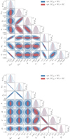 |
Fig. A.1. Top panel: 1σ and 2σ confidence contours on the optimistic, flat GR case for GCph+WL (blue) vs. GCph+WL+XC (red) for the seven cosmological parameters, using the Flagship bias as a fiducial galaxy bias model. Bottom panel: 1σ and 2σ confidence contours on the optimistic, flat GR case for GCph+WL (blue) vs. GCph+WL+XC (red) for the IA parameters and the four bias parameters, using the same galaxy bias model as above. |
68% errors on the ten bias parameters of the binned bias model with and without the XC contribution.
68% errors on the cosmological parameters of the binned bias model with and without the XC contribution.
68% errors on the ten bias parameters of the binned bias model with and without the XC contribution.
68% errors on the cosmological parameters, with and without the XC contribution, when the bias is modeled following the Flagship simulation.
All Tables
Summary of nuisance parameters considered in this analysis together with their fiducial values.
Constraint on the IA nuisance parameters for flat and non-flat cases for both the pessimistic and optimistic assumptions.
68% errors, without and with the XC contribution, on the nuisance parameters (both bias and IA) when the Flagship bias model is considered.
68% errors on the ten bias parameters of the binned bias model with and without the XC contribution.
68% errors on the ten bias parameters of the binned bias model with and without the XC contribution.
68% errors on the cosmological parameters of the binned bias model with and without the XC contribution.
68% errors on the ten bias parameters of the binned bias model with and without the XC contribution.
68% errors on the cosmological parameters, with and without the XC contribution, when the bias is modeled following the Flagship simulation.
All Figures
|
Fig. 1. Different bias parameterisations used in the paper: the binned bias (orange line) and the Flagship bias (red line), for the fiducial values of their respective parameters. Also shown are the measurements of the galaxy bias in the Flagship simulation (black dots). For illustrative purposes, a further 25 lines for each case are represented alongside the fiducials, showing how the galaxy bias changes when we allow for a Gaussian dispersion of 5% on the bias nuisance parameters. |
| In the text | |
|
Fig. 2. Ratio of the marginalised (top panel) and unmarginalised (bottom panel) forecast uncertainties on the bi bias parameters between WL+GCph and WL+GCph+XC, in the pessimistic (red lines) and optimistic (yellow lines) cases. We show in this plot results for both the flat Universe model (solid lines) and the non-flat case (dashed lines). |
| In the text | |
|
Fig. 3. 1σ and 2σ confidence contours on the optimistic, flat GR baseline case for GCph+WL (orange) vs. GCph+WL+XC (green) for the three intrinsic alignment parameters compared to the Ωm, 0 parameter. While the IA parmeters are clearly highly degenerate among themselves, Ωm, 0 shows little degeneracy with them, especially when XC is included. |
| In the text | |
|
Fig. 4. 1σ and 2σ confidence contours on the optimistic, flat, modified gravity baseline case for GCph+WL (orange) vs. GCph+WL+XC (green). The modified gravity parameter γ is not significantly better constrained when including XC, but its inclusion helps to break some degeneracies, especially with w0, wa, and σ8. |
| In the text | |
|
Fig. 5. Shifts in units of standard deviations for Ωm, 0 (left panel), w0 (middle panel), and wa (right panel) due to an incorrect assumption on the IA amplitude. Results are shown for the optimistic case with WL+GCph (orange) vs. WL+GCph+XC (green). Solid (dashed) lines represent positive (negative) shifts with respect to the fiducial. The vertical grey line shows the case in which we assume no contribution from IA (𝒜IA = 0). The grey-shaded region denotes the shifts larger than 3σ, for which the Gaussian approximation breaks down and the corresponding shifts should be interpreted with caution (see the text for details). |
| In the text | |
|
Fig. 6. Difference between the FoM and the reference one obtained in the case where all shifts in the mean of the photometric-redshift distributions are perfectly known and equal to zero (Δzi = σ(Δzi) = 0), for a changing value of the prior added. The results refer to GCph (red), WL (purple), WL+GCph (orange), and WL+GCph+XC (green), under pessimistic (dashed) and optimistic (solid) assumptions. The black dot denotes the prior threshold for which the final FoM of the full WL+GCph+XC combination in the optimistic case is degraded by 20%. The black triangle represents the same threshold in the pessimistic case (see the text for details). We note that the reference FoM is larger for the optimistic case in comparison to the pessimistic case, and it increases when the XC terms are included. However, the different lines are normalised to their corresponding reference FoMs for illustrative purposes. |
| In the text | |
|
Fig. 7. Ratio of the errors on Δzi with and without the inclusion of XC. Yellow and red lines refer to the pessimistic and optimistic scenario. |
| In the text | |
|
Fig. A.1. Top panel: 1σ and 2σ confidence contours on the optimistic, flat GR case for GCph+WL (blue) vs. GCph+WL+XC (red) for the seven cosmological parameters, using the Flagship bias as a fiducial galaxy bias model. Bottom panel: 1σ and 2σ confidence contours on the optimistic, flat GR case for GCph+WL (blue) vs. GCph+WL+XC (red) for the IA parameters and the four bias parameters, using the same galaxy bias model as above. |
| In the text | |
Current usage metrics show cumulative count of Article Views (full-text article views including HTML views, PDF and ePub downloads, according to the available data) and Abstracts Views on Vision4Press platform.
Data correspond to usage on the plateform after 2015. The current usage metrics is available 48-96 hours after online publication and is updated daily on week days.
Initial download of the metrics may take a while.