| Issue |
A&A
Volume 642, October 2020
|
|
|---|---|---|
| Article Number | A229 | |
| Number of page(s) | 16 | |
| Section | Planets and planetary systems | |
| DOI | https://doi.org/10.1051/0004-6361/202038767 | |
| Published online | 23 October 2020 | |
Connecting planet formation and astrochemistry
C/Os and N/Os of warm giant planets and Jupiter analogues
1
Leiden Observatory, Leiden University,
2300
RA Leiden, The Netherlands
e-mail: This email address is being protected from spambots. You need JavaScript enabled to view it.
2
Max-Planck-Institut für Extraterrestrishe Physik,
Gießenbachstrasse 1,
85748
Garching, Germany
3
Department of Physics and Astronomy, McMaster University,
Hamilton,
Ontario,
L8S 4E8, Canada
4
Origins Institute, McMaster University,
Hamilton,
Ontario,
L8S 4E8, Canada
Received:
26
June
2020
Accepted:
5
September
2020
Abstract
The chemical composition of planetary atmospheres has long been thought to store information regarding where and when a planet accretes its material. Predicting this chemical composition theoretically is a crucial step in linking observational studies to the underlying physics that govern planet formation. As a follow-up to an earlier study of ours on hot Jupiters, we present a population of warm Jupiters (semi-major axis between 0.5 and 4 AU) extracted from the same planetesimal formation population synthesis model as used in that previous work. We compute the astrochemical evolution of the proto-planetary disks included in this population to predict the carbon-to-oxygen (C/O) and nitrogen-to-oxygen (N/O) ratio evolution of the disk gas, ice, and refractory sources, the accretion of which greatly impacts the resulting C/Os and N/Os in the atmosphere of giant planets. We confirm that the main sequence (between accreted solid mass and the atmospheric C/O) we found previously is largely reproduced by the presented population of synthetic warm Jupiters. As a result, the majority of the population falls along the empirically derived mass-metallicity relation when the natal disk has solar or lower metallicity. Planets forming from disks with high metallicity ([Fe/H] > 0.1) results in more scatter in chemical properties, which could explain some of the scatter found in the mass-metallicity relation. Combining predicted C/Os and N/Os shows that Jupiter does not fall among our population of synthetic planets, suggesting that it likely did not form in the inner 5 AU of the Solar System before proceeding into a Grand Tack. This result is consistent with a recent analysis of the chemical composition of Jupiter’s atmosphere, which suggests that it accreted most of its heavy element abundance farther than tens of AU away from the Sun. Finally, we explore the impact of different carbon refractory erosion models, including the location of the carbon erosion front. Shifting the erosion front has a major impact on the resulting C/Os of Jupiter- and Neptune-like planets, but warm Saturns see a smaller shift in C/Os since their carbon and oxygen abundances are equally impacted by gas and refractory accretion.
Key words: planets and satellites: atmospheres / planets and satellites: formation / planets and satellites: gaseous planets / astrochemistry
© ESO 2020
1 Introduction
It is now well established that the study of an exoplanetary atmospheric carbon-to-oxygen ratio (C/O) represents an important step in understanding the physical processes that govern planet formation (Öberg et al. 2011; Helling et al. 2014; Madhusudhan et al. 2014; Cridland et al. 2016, 2019a). To date, measurements of the atmospheric C/O have largely been carried out for hot Jupiters and hot Neptunes because their proximity to their host star makes high signal-to-noise transmission and emission spectra more easily attainable (Madhusudhan 2012; Moses et al. 2013; Brogi et al. 2014; Line et al. 2014; Brewer & Fischer 2016; Gandhi & Madhusudhan 2018; Pinhas et al. 2019; MacDonald & Madhusudhan 2019).
Cold Jupiters (a.k.a. directly imaged planets) are located farther away from their host stars and have orbital radii ≥8 AU, which can be chemically characterized through the efforts of direct spectroscopy and interferometry. The GRAVITY consortium, with their recent effort for β Pic b (at 9.2 AU, GRAVITY Collaboration 2020), has provided a precise measurement of the C/O for that planet and has shown that such a measurement is feasible with the interferometric mode of the Very Large Telescope (VLT, see also GRAVITY Collaboration 2019). This method of chemical characterization will compliment the efforts of the direct-imaging community, which has planned both Early Release Science1 and Guaranteed Time Observations2 with the James Webb Space Telescope (JWST) for planets at farther distances.
At orbital radii between the hot and cold Jupiters are a population of exoplanets that have not been well studied chemically. These “warm” Jupiters are defined as having orbital radii between 0.5 and 10 AU. They orbit too close to their host star to be detectable by direct imaging and far enough away that their detection via the transit method is limited due to their long orbital periods. With this definition, Jupiter and Saturn, with effective temperatures of 134 and 97 K, respectively (Aumann et al. 1969), are classified as warm Jupiters. We note that this classification is not based on the effective temperature of the planet (which can depend strongly on internal processes), but instead only depends on the planet’s orbital radius.
In Fig. 1, we show the population of known exoplanets coloured by their primary discovery method3. Additionally, we outline the mass and orbital radius range that is relevant for warm Jupiters with black lines. The majority of these planets were discovered through the radial velocity and microlensing techniques, with a few discovered through primary transits, astrometry, and direct imaging. As already mentioned, these planets exist in a region of parameter space that makes their chemical characterization difficult, and as such there are few examples where such a measurement has been attempted. Regardless, occurrence rate studies of giant planets have shown that Jupiter analogues (giant planets orbiting between 3 and 6 AU) should be more abundant (~ 3.3% of stars, Wittenmyer et al. 2011)than hot Jupiters (~1.2% of stars, Wright et al. 2012). This conclusion, which is supported by population synthesis studies (Mordasini et al. 2009; Hasegawa & Pudritz 2013; Chambers 2018), motivates our study of warm Jupiters.
To what extent can the chemical properties of Jupiter and Saturn be understood in the context of the warm Jupiters? While how Jupiter and Saturn formed are still open questions, there are two leading formation scenarios that have been studied in the literature: planetesimal accretion near the water ice line (Pollack et al. 1996; Alibert et al. 2005; Helled et al. 2014) and pebble accretion (Bitsch et al. 2015; Bosman et al. 2019). Comparing the chemical properties of our modelled warm Jupiters to Jupiter and Saturn can help differentiate between these different formation pathways. Another popular planet formation scenario is gravitational instability, which is thought to lead to planets on wider orbits than our giant planets (see for example Dodson-Robinson et al. 2009).
If Jupiter and Saturn formed through planetesimal accretion near the water ice line, then they would have to undergo a Grand Tack (Walsh et al. 2011) to migrate out to their current orbital radius (from 1–3 AU to 5.5 and 9.5 AU, respectively). This process, however, is highly sensitive to the mass ratio of the two planets and requires a particular orbital radius arrangement to function (Raymond & Morbidelli 2014; Chametla et al. 2020). In this way, there could be many solar systems in the galaxy that have planets that underwent formation histories similar to that of Jupiter but did not undergo a Grand Tack. Our simulated population of warm Jupiters orbit at radii smaller than 4 AU (see below) and hence can be thought of as Jupiter and Saturn analogues that did not undergo a Grand Tack.
This work is a follow-up to our previous work that studied the chemistry of a population of hot Jupiters (Cridland et al. 2019b, Paper I). The population we study here is extracted from the same population synthesis model as our hot Jupiter model in Paper I (taken from Alessi et al. 2020). In Paper I, we found a relation between the atmospheric C/O in these hot Jupiters and the fraction of their total mass that was accreted as solids. We dubbed this relation a “main sequence” of the atmospheric C/O and highlighted the fact that solid accretion – as planetesimals in our model – are important for determining the bulk chemical properties of hot Jupiter atmospheres. The well-known (empirically derived) mass-metallicity relation (Kreidberg et al. 2014) directly follows from this main sequence. Its prediction – that higher-mass planets have lower bulk metallicity – is explained by our main sequence as being caused by the fact that high-mass planets tend to be more dominated by gas accretion than solid accretion.
Does this main sequence – and hence the mass-metallicity relation – continue to work for warm Jupiters? And can the chemical structure of Jupiter’s atmospheres (and by extension its formation history) be explained by our planetesimal accretion model? Unlike hot Jupiters, the orbital radii of warm Jupiters range across large chemical gradients in the disk, including the water ice line (between 2 and 4 AU) and the carbon erosion front (~ 5 AU). As such, we expect to find a larger spread in atmospheric chemical compositions than we did in Paper I. On the other hand, hot Jupiters are expected to have undergone a long history of orbital migration. As such, the two sub-populations could have accreted the bulk of their gas in similar locations in the disk, and while hot Jupiters migrated very close to their host stars, warm Jupiters did not. In this case, we might expect very little chemical difference between the two types of planets.
In what follows, we run a similar method to what was reported in Paper I. We compute the astrochemical evolution in the proto-planetary disks that produce each of the warm Jupiters in our model. We then track the abundances of carbon, oxygen, and nitrogen that are available to be accreted into the planetary atmosphere from the disk gas, ice, and refractory sources. We derive the resulting elemental ratios and analyze the connection between these ratios and the physical properties that govern planet formation. We briefly outline our method in Sect. 2, report our results in Sects. 3–5, and discuss the implication on understanding Jupiter analogues in Sect. 6. We conclude on this study in Sect. 7.
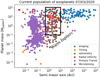 |
Fig. 1 Current population of confirmed exoplanets extracted on March 7, 2020 (from exoplanet.eu). We note the range of masses and semi-major axes that define our warm Jupiters with black lines. The majority of planets in this range were discovered through direct imaging, radial velocity, and microlensing. |
2 Method: combining astrochemistry and planet formation
As discussed in Paper I, the main feature of our work is the combination of evolving astrochemical models of proto-planetary disks with a planetesimal accretion model. In this way, we can prescribe the chemical properties (abundances of carbon, oxygen, and nitrogen) in the gas, ice, and refractory components of the proto-planetary disk at the same time and place as the growing proto-planet. The population synthesis model that produced our population of planets is described in Alessi et al. (2020). The chemical kinetic code that predicts the gas and ice composition of the disk is based on the work of Fogel et al. (2011) and Cleeves et al. (2014), but it has been modified for our purposes as described in Paper I. The chemical model that describes the chemical composition of the refractory component (dust and planetesimals) was introduced in Cridland et al. (2019a) and includes the possibility of carbon erosion in the inner disk. We outline some of the important concepts here; more details are available in Cridland et al. (2019b) and Alessi et al. (2020).
2.1 Planet growth and migration
As a planet grows, it evolves through the mass-semi-major axis diagram in Fig. 1 through a combination of solid accretion followed by gas accretion (increasing vertically in Fig. 1) and through planetary migration (decreasing horizontally in Fig. 1). Alessi et al. (2020) used the planetesimal accretion paradigm (Pollack et al. 1996; Ikoma et al. 2000; Kokubo & Ida 2002; Ida & Lin 2004; Alibert et al. 2005) to build the initial planetary core.The rate of growth is dictated by the surface density of planetesimals, which we take as being equal to the dust surface density at any given time. Our dust surface density evolves according to the semi-analytic model of Birnstiel et al. (2012), primarily through radial drift that quickly empties the outer disk of dust4.
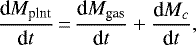
Planetesimal formation dictates that the core growth rate is (Pollack et al. 1996):
![Mathematical equation: \begin{align*} \frac{\textrm{d}M_{\textrm{plnt}}}{\textrm{d}t} \,&{=}\, \frac{\textrm{d}M_c}{\textrm{d}t}\,{=}\,\frac{M_c}{\tau_{c,\textrm{acc}}} \nonumber\\ \simeq & \frac{M_c}{1.2\times 10^5} \left(\frac{\Sigma_{\textrm{dust}}}{10\,\textrm{g\,cm}^{-2}}\right)\left(\frac{a}{1 \,\textrm{AU}}\right)^{-1/2} \left(\frac{M_c}{M_{\oplus}}\right)^{-1/3}\left(\frac{M_s}{M_{\odot}}\right)^{1/6} \nonumber\\ \ \ \times& \left[\left(\frac{\Sigma_{\textrm{gas}}}{2.4\times 10^3 \textrm{g\,cm}^{-2}}\right)^{-1/5} \left(\frac{a}{1\,\textrm{AU}}\right)^{1/20}\left(\frac{m}{10^{18}\,\textrm{g}}\right)^{1/15}\right]^{-2} \textrm{g~yr}^{-1}\end{align*}](/articles/aa/full_html/2020/10/aa38767-20/aa38767-20-eq1.png) (1)
(1)
for a planet core of mass Mc currently orbiting at a around a star of mass Ms and accreting planetesimals of (an assumed constant) mass m. The solid surface density Σdust is determined from the Birnstiel et al. (2012) model, while the gas surface density Σgas is determined from a semi-analytic model based on Chambers (2009)5.
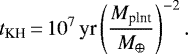
Once the planet is sufficiently large, it clears the majority of its “feeding zone” of planetesimals, and core growth is drastically slowed (Ida & Lin 2004)6. Particularly since the planet migrates through the disk, it can continue to accrete planetesimals into its proto-atmosphere, delivering any carbon and oxygen contained within the planetesimal (see below). Due to the reduced planetesimal accretion rate, the core begins to cool – which enables a stage of gas accretion to begin (Ikoma et al. 2000). Gas accretion begins at a very slow rate, limited by the Kelvin-Helmholtz timescale (Ida & Lin 2004) such that the mass of the planet evolves as:
 (2)
(2)
where dMgas∕dt = Mplnt∕tKH, and dMc∕dt proceeds at the aforementioned reduced rate. The Kelvin-Helmholtz timescales with the total mass of the planet (Ikoma et al. 2000; Alessi & Pudritz 2018) are:
 (3)
(3)
In the population synthesis model of Alessi et al. (2020), gas accretion is assumed to halt when the planet reaches some final mass. This final mass is proportional to the gap opening mass with a proportional constant that is generated from a log-normal distribution as part of the population synthesis model. While the general problem of late stage gas accretion remains unsolved, our approach captures the essential points of more complex physical models of the end state of gas accretion (see, for example, D’Angelo et al. 2010; Cridland 2018).
The population synthesis model of Alessi et al. (2020) stochastically selects a set of the initial disk mass, disk lifetime, and metallicity to initialize the radial distribution of the gas and dust surface densities and the gas temperature as well as to control the evolution of the disk’s mass accretion rate. The initial disk (gas) mass and disk lifetime are selected from a log-normal distribution with an average of 0.1 M⊙ and 3 Myr, respectively. Their distributions have a 1σ range of 0.073–0.137 M⊙ and 1.8–5 Myr, respectively. The disk metallicity ([Fe/H])7 is selected from a normal distribution with an average of −0.02 (marginally sub-solar) and a 1σ range of −0.22–0.18. The disk metallicity sets the initial gas-to-dust ratio using the expression:
![Mathematical equation: \begin{align*} f_{\textrm{gtd}}\,{=}\,f_{\textrm{gtd,0}}10^{\textrm{[Fe/H]}}, \end{align*}](/articles/aa/full_html/2020/10/aa38767-20/aa38767-20-eq4.png) (4)
(4)
where fgtd,0 = 0.01 is the typical interstellar medium (ISM) gas-to-dust ratio, such that the radial distribution of dust mass is:
 (5)
(5)
where Σgas is derived from the disk model of Chambers (2009). Changes in the initial dust surface density impact the rate of the initial core growth through the availability of core-building material at a given ratio.
In Paper I, we derived the total mass evolution for the set of generated disks and compared them to recent observational surveys of young stellar systems. We found that the population of disks used by Alessi et al. (2020) reproduced the high-mass end of the observed population of proto-planetary disks and generally agreed better with the population of Class 0/I objects from Tychoniec et al. (2018). In this way, our generated disks can be thought of as beginning marginally Class I objects (similar to HL Tau, ALMA Partnership 2015) when we start planet formation, although we ignore the impact of any remaining envelope.
As previously mentioned, growing planets migrate to smaller orbital radii through interactions with the proto-planetary disk gas (Lin & Papaloizou 1986; Ward 1991). Planet migration has been an ever-growing topic since it was first pointed out that the typical timescale for Type I migration (for low-mass planets that do not open gaps) is too short, compared to the typical planetesimal accretion timescale, to explain the known population of exoplanets (Ward 1997). A way to remedy this discrepancy is to either slow planetary migration or speed up planetary accretion. The former solution, typically called “planet trapping”, posits that discontinuities in the gas density, temperature, or dust opacity can lead to a change in the strength of the torques responsible for migration (Masset et al. 2006). This change can slow the migration rate, stop it completely, or even reverse its direction (Masset et al. 2006; Hasegawa & Pudritz 2010, 2011; McNally et al. 2018, 2020).
In our planet formation model, we used the three planet traps outlined in Hasegawa & Pudritz (2011) – the water ice line, the dead zone edge, and the heat transition – to dictate where the growing planet must be, up until the point where it opens a gap in the disk (discussed below). The particular trap that houses a given planet dictates where that planets begins its core formation. The typical hierarchy states that the water ice line is the most inward trap followed by the dead zone and then the heat transition beginning the farthest from the host star. The farther fromthe host star a planet begins, the less material is available for core growth, slowing this initial phase of accretion.
Each of the aforementioned planet traps rely on a different transition in the properties of the disk. The water ice line is a transition in the dust opacity located at the sublimation temperature (typically ~ 170 K) of water ice. At lower temperatures, water is frozen out onto the dust grains, and their resulting opacity is larger than at higher temperatures where the water is in its vapour phase. Cridland et al. (2019c) investigated this process in detail and confirmed that such a transition does indeed create a planet trap for the water ice line. Additionally, in Cridland et al. (2019c), the dead zone edge (which represents a transition in the disk turbulent α) and the heat transition (where the primary heating mechanism changes from viscous to direct irradiation, Hasegawa & Pudritz 2010; Lyra et al. 2010) are tested and similarly found to produce planet traps. All three of these traps evolve to smaller radii as the disk loses mass due to its own accretion onto the host star and cools as a result. Hence proto-planets continue to move inwards as they grow, but on a much longer timescale (the viscous timescale) than in the standard picture of Type I migration.
Once the planet is sufficiently large, it opens a gap in its disk (Crida 2009). At this point, Type I migration is suppressed and is replaced by Type II migration (Lin & Papaloizou 1986). During this stage of planetary migration, the planet acts as an intermediary for the angular momentum transport through the disk and generally migrates inwards on the viscous timescale. As we outlined in Paper I, when the mass of the planet exceeds the gap opening mass, we assume that its radial evolution proceeds on the viscous timescale.
Apart from adjusting the rate of migration, other methods of saving planets from this “Type I problem” have been proposed. These include pebble accretion, which posits that the core initially grows through the accretion of cm-sized pebbles – a process that can increase the rate of initial core growth by a factor of ~ 1000 (Ormel & Klahr 2010; Lambrechts & Johansen 2014; Bitsch et al. 2015). Another method involves the direct gravitational collapse of giant planets through an instability at hundreds of AU in the proto-planetary disk. While not necessarily faster than core accretion, starting from such large disk radii ensures that there is insufficient time for the growing planet to migrate into the host star.
A final method could simply be starting planet formation earlier than previously assumed. Recent surveys of proto-planetary disks (also known as Class II objects) have shown that there is currently insufficient dust (by 1–3 Myr) available to produce the core of a Jupiter-like planet, let alone multiple planets (Ansdell et al. 2016; Manara et al. 2018; Tychoniec et al. 2018, 2020). Younger Class 0/I objects, however, have been found to contain at least 20 times more dust than Class II objects (Tychoniec et al. 2020). This finding suggests that (at the very least) there is significant planetesimal formation ongoing in young stellar systems. Planets forming in these systems would likely undergo planet migration; however, due to the complex nature of these embedded systems, the relevant torques have not yet been characterized.
Here we continue to use the planetesimal accretion and migration prescriptions developed in our past work (Hasegawa & Pudritz 2013; Alessi et al. 2017; Cridland et al. 2016). We will leave the implications of the aforementioned models to future work.
2.2 Astrochemistry of the volatiles and refractories
2.2.1 Volatiles
We include an astrochemical model for the evolution of both the volatile and refractory components of the disk carbon, oxygen, and nitrogen. The volatile component of the disk is primary made up of H2O, CO2, and CO gasand ice frozen onto dust grains. The disk volatile evolution is computed using the Michigan chemical kinetic code featured in Fogel et al. (2011) and Cleeves et al. (2014), and previously used in Cridland et al. (2016, 2017a). It computes the disk chemistry in a 1+1D fashion, assuming vertically isothermal gas and dust as well as hydrostatic equilibrium. The chemical evolution is initialized with elemental ratios O/Hvol = 2.5 × 10⁻⁴, C/Hvol = 1.0 × 10⁻⁴, and N/Hvol = 2.45 × 10⁻⁵ assuming an inheritance scenario. In this scenario, the carbon and oxygen begin in their molecular form (largely CO and frozen H2O), while nitrogen is initialized primarily in atomic N with ~10% molecular N2. Under these conditions, the volatile C/O = 0.4 and N/O = 0.098. The cosmic ray induced ionization rate is 1 × 10⁻¹⁷ s−1.
The chemical interaction between the dust grain surface and the gas represents a crucial driver for chemical change. The chemical network underlying the Michigan chemical code includes a limited set of grain surface reactions, primarily focused on the production of molecular hydrogen and water. More complex grain surface reactions involving carbon-bearing species (as seen in Walsh et al. 2015; Eistrup et al. 2018; Bosman et al. 2018; Krijt et al. 2020) are left out of the chemical model as they typically become relevant at lower temperatures, outside the CO2 ice line (~ 10 AU). None of our forming warm Jupiters build their atmospheres that far out in the disk. We compute an average dust grain size for our chemical calculation based on the output from the a semi-analytic model of dust evolution (Birnstiel et al. 2012), weighted by the number density of dust grains. An implementation of this method is presented in Cridland et al. (2017a); the typical average grain size is ~ 0.1μm.
The version of the Michigan code that was used in the aforementioned works assumed a passive disk model that remains unchanged over the whole evolution of the chemical system. In Paper I, we introduced a new version of the code that allowed the disk gas density and temperature to evolve in tandem with the chemistry. This new method introduced new chemical features that did not appear in the passive version of the code (see Paper I).
2.2.2 Refractories
A large reservoir of carbon and oxygen also exists in refractory sources – planetesimals and pebbles – in proto-planetary disks (Pontoppidan et al. 2014). These refractory sources are effectively chemically neutral and do not contribute to the bulk elemental abundances inferred by (sub)millimetre studies of proto-planetary disks. A possible exception to this trend is carbon; there has been evidence found in our own Solar System for an interaction between refractory and volatile sources of the element (Bergin et al. 2015). Given that the carbon-to-silicon ratio (C/Si) of the ISM is approximately six, and assuming that the majority of the silicates have the SiO3 group, then the refractory C/O = 2. As such, their accretion into the atmospheres of giant planets could have a drastic impact on the resulting C/O (as discussed in Cridland et al. 2019a). We assume that there is no refractory component for nitrogen.
The Earth is depleted in carbon (relative to silicon) by three orders of magnitude when compared to the C/Si of the ISM. Moreover, main-belt asteroids show between one and two orders of magnitude depletion in their C/Si relative to the ISM. This depletion prompted Bergin et al. (2015) to propose that some chemical process was eroding the carbon from the dust early in the life of our natal disk, consequently enhancing the gas phase carbon. The chemical processes responsible were investigated by Lee et al. (2010), Anderson et al. (2017), and Klarmann et al. (2018), but no concrete answer was found. The chemical implication of such a process was investigated by Wei et al. (2019). They find that the majority of the excess carbon stayed in the gas phase as HCN and hydrocarbons, with only ~ 1% of the carbon condensing back onto the grains in the form of icy long-chain hydrocarbons.
We included an analytic prescription that describes the distribution and evolution of carbon from the refractory sources into the gas phase. The distribution of the excess gaseous carbon was derived in Cridland et al. (2019a) and was based on an empirical fitto Solar System data by Mordasini et al. (2016). There are two models that describe the distribution of excess carbon: the “reset” and “ongoing” models. As outlined in Cridland et al. (2019a), these models represent simple but opposing methods for eroding the carbon from the dust grains into the gas. The reset model assumes that during the initial collapse of the molecular cloud a thermal event – similar to an FU Ori outburst – sublimates the dust in the young proto-planetary disk, releasing its contents into the gas phase. As the disk returns to its natural temperature, the silicates and iron recondense into dust, but the carbon does not. This model assumes that all the erosion necessary to explain the current depleted C/Si of Earth and main-belt asteroids happens at (effectively) t = 0. The carbon released due to this process would then advect along with the rest of the gas and dust in the disk into the host star.
The opposing model, the ongoing model, assumes that there is some ongoing chemical process that is continually eroding carbon fromdust grains in the proto-planetary disk. This process – while not concretely identified – would continually maintain the excess carbon in the disk as carbon-rich dust grains radially drift into the region of the disk where the erosion can happen (a few AU, Anderson et al. 2017). The main difference between these two models is that the excess carbon vanishes in the reset model after less than 1 Myr (Cridland et al. 2019a, but also see Fig. 2), while the excess carbon survives the full lifetime of the disk in the ongoing model.
2.2.3 General chemical evolution and the carbon erosion front
In Fig. 2, we show the radial distribution and evolution of the midplane C/O for both the gas and the solids (ice and refractories) for a single disk model over a span of just over 1 Myr. We note a few points of interest: first, we have included the reset model from Cridland et al. (2019a), which greatly enhances the gaseous carbon content at the expense of carbon from the refractory component. By approximately 0.8 Myr, the extra carbon has completely moved into the host star and is no longer available to accrete into any forming proto-planets. Had the ongoing model been included in Fig. 2, the carbon-rich region A would have extended over all times in much the same way as the carbon-poor region E does in the right-hand panel. We note that both the reset and ongoing models result in the carbon-poor region E because they both lead to the required depletion in refractory carbon seen currently in the inner Solar System. In our model, there is a particular radius where the solids transition between being carbon-rich and carbon-poor. This radius is known as the carbon erosion front and is located at 5 AU in the fiducial carbon erosion model. The location of the front remains fixed in the ongoing model so that the excess carbon in the gas phase perfectly reflects the depletion of carbon in the solid phase (transition radius between regions E and F). In the reset model, since the excess carbon advects with the bulk gas in the proto-planetary disk, the erosion front representing the excess gaseous carbon moves inwards. This evolution can be seen in Fig. 2 as the curved white contour between regions A and B. Later in this work, we explore the impact of varying the location of this erosion front.
When the extra carbon due to the reset refractory erosion model advects away from a given disk radius, the gas is returned to a lower C/O, which is indicative of the initial C/O used in our chemical model (0.4). In region B, the final C/O that was used as the initial condition can be found inside the water ice line. This region slowly shrinks as the disk cools, and the water ice line moves inwards. Outside the water ice line in region D, water is primarily in the ice phase, which brings the gas C/O up to a value closer to unity. The carbon- and oxygen-carrier molecules are dominated by CO in this region since we only include CO2 production in the gas phase – which is generally much less efficient than it is in the ice phase (as discussed in Paper I). We do see a short period of CO2 production in region C, which is produced in the gas before quickly freezing out onto the dust grains at the cost of frozen H2O and gaseous CO. As such, there is a local decrease in the C/O with a subsequent increase in the C/O in the solids. This process has already been explored by Eistrup et al. (2016) and was similarly observed in Cridland et al. (2019b). However, the process only lasts for a few 105 yr before the disk becomes too cold in that region for it to occur efficiently. The slightly more carbon-rich region just below C is caused by a small quantity of HCN and long-chain hydrocarbons being produced in the gas phase. We show all of the most abundant gas and ice species in Figs. A.1 and A.2, respectively.
While the left-hand panel of Fig. 2 shows the C/O for the gaseous disk, the right-hand panel shows the C/O for the solids. This panel includes the C/O for both the ice and refractory sources (dust and planetesimals), but it is dominated by the refractory sources (apart from the small feature mentioned above). This is why it shows much less structure than in the left-hand panel - including the decrease in the C/O that would accompany the increases seen between regions B and D in the left-hand panel. Instead, it mainly shows the transition region inside the carbon erosion front – the radius where we assume the erosion begins. The carbon refractory erosion model assumes ISM values of carbon (C/Href = 2.4 × C/Hvol) outside the carbon erosion front (assumed to be 5 AU in our fiducial model, more below), while rapidly and smoothly depleting the carbon by a factor of 1000 within 5 AU. The functional form of this erosion model was derived empirically by Mordasini et al. (2016) and is shown in Cridland et al. (2019a).
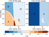 |
Fig. 2 Evolution and radial distribution of the midplane C/O in the gas and solids in one of the disk models used for this work. Specifically, we show the chemistry of the disk in the reset scenario of refractory erosion, which governs the high C/O early on in the disk’s life (A). We similarly note the region of the disk with high and low water vapour abundances (B and D, respectively), the carbon-poor region due to refractory erosion (E), and a region where gaseous CO is converted to frozen CO2 (C). The more carbon-rich region (F) exists at larger radii than the carbon erosion front. Orange denotes carbon-rich regions (C/O > 1) while blue denotes carbon-poor regions (C/O < 1). The nominalvolatile C/O = 0.4 and the refractory C/O = 2. |
2.2.4 Chemical accounting in planetary atmospheres
As already discussed, the proto-planetary disk has two sources of carbon, oxygen, and nitrogen for the growing proto-planet. If the gas accretes onto the planet at a rate of dMgas∕dt, then the total rate of change of any element is simply:
 (6)
(6)
where X∕H is the abundance of element X relative to hydrogen as computed by our chemical model (volatiles and carbon erosion combined), and μmH is the average weight of a gas particle. In principle, micron-sized dust grains will be accreted into the atmosphere along with the gas since they are well coupled. However, along the midplane of the disk (from where we assume the material is accreted), these grains make up a very small fraction of the total mass of the dust (less than 0.1%).
Recently, Cridland et al. (2020) explored the impact of vertical accretion on the chemical composition of exoplanetary atmospheres; they find that the micron-sized grains can play a role but only if material is accreted from between one and three gas scale heights. In that case, the grains typically bring oxygen-rich ices to the growing planet, generally lowering the atmospheric C/O. For simplicity, we ignore the impact of vertical accretion and hence assume that the micron-sized grains do not contribute to the total mass of the planet nor the chemical structure of its atmosphere.
Conversely, we do account for the mass of carbon and oxygen frozen or locked in refractories of the planetesimals that accrete into the proto-atmosphere. For this, we follow the work of Cridland et al. (2019a) with a simple prescription based on the more detailed calculations of planetesimal survival in planetary atmospheres of Mordasini et al. (2015). We chose an atmospheric mass cutoff of 3 M⊕, below which an incoming planetesimal survives its trip through the atmosphere and delivers its refractory material directly to the core8. The planetesimal should, however, heat up sufficiently to release any volatiles incorporated in the form of ice. We assume that all volatile (ice) species are released as the planetesimal passes through the atmosphere.
When the atmospheric mass exceeds 3 M⊕, Mordasini et al. (2015) show that planetesimals (regardless of initial size) will completely evaporate in the atmosphere. For planets that exceed this atmospheric mass, we assume that all refractory mass is released and efficiently mixed throughout the atmosphere - thereby impacting the bulk C/O of the planet. We follow Mordasini et al. (2016) in assuming that the relative mass fractions are 2:4:3 for carbon (in regions with no carbon erosion), silicates, and irons, respectively. As such, silicates make up 4/9 of the planetesimal mass in regions with no carbon erosion and 4/7 of the mass in regions where the carbon has eroded.
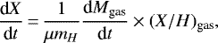
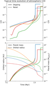 |
Fig. 3 Typical evolution of the atmospheric C/O as a proto-planet grows (top panel). We show the results for each of the example planets for each of the ongoing (solid line) and reset (dashed line) carbon erosion models. In addition, we show the mass and orbital radius evolution of the same planets (bottom panel). |
3 Results: individual formation and chemical inheritance
To get a sense for the typical evolution of the C/O in our growing planets, we show, in Fig. 3, the temporal evolution of the C/O (top panel) with the orbital radius and the planet mass (bottom panel). The planets begin their evolution as large planetary embryos with M = 0.01 M⊕. They slowly build up solid mass by accreting planetesimals and a small amount of a gas envelope, building up an initial core of M ~ 10 M⊕ in ~ 0.5 Myr. At this point, the growing planet is slowly accreting gas and any remaining planetesimals (discussed above). By ~ 1 Myr, the embryosare sufficiently large to begin to quickly accrete gas, eventually doing so in an unstable manner. Once the planet has reached its prescribed maximum mass (chosen from a distribution prior to each calculation), its evolution is stopped.
During the initial build-up of the core the “atmospheric” C/O9 is dominated by the release of volatiles that had been frozen onto incoming planetesimals as they pass through the early proto-atmosphere. Planets forming near or inside the water ice line are under-abundant in volatiles but can contain small amounts of hydrocarbons. These, when combined with the small amount of gas (which is rich in water vapour) that is accreted at this stage, leads to the low atmospheric C/O for the first ~Myr. Planets forming outside the water ice line accrete planetesimals rich in frozen water, which drives the very low initial C/O. All four of these planets grow in the transition region of the carbon erosion model, meaning that planets that form closer to the host star accrete planetesimals with less carbon than planets that form farther away. Once their proto-atmosphere is sufficiently large, refractories begin to contribute to the atmospheric C/O and hence planets forming farther away (green line) see a steeper increase in their C/O than planets closer in (red and blue lines) after ~ 0.5 Myr. Because it forms outside the water ice line, the planet denoted by the orange line sees its C/O slightly reduced prior to the beginning ofmore rapid gas accretion.
Once gas accretion starts to dominate the mass evolution, the atmospheric C/O begins to evolve towards the local C/O of the proto-planetary disk; this includes the impact of the carbon erosion model. In the case of the reset model (dashed line), the atmospheric C/O evolves towards ~ 0.4 inside the water ice line (green and red lines) and ~0.7 outside the water ice line (blue line). Planets accreting in short-lived disks (orange line) are stranded at lower C/Os because their gas accretion is halted by the photo-evaporating disk. In the case of the ongoing model, there is extra carbon in the gas that is accreted by the growing planets, enhancing their atmospheric C/O.
Because of the unstable gas accretion in our formation model, most of the C/O evolution happens over a short period of time as the bulk of the atmosphere is accreted. As such, giant planets freeze in the chemical composition of the gas at their location in the proto-planetary disk where their unstable gas accretion occurred. Lower-mass planets (orange line) do not undergo unstable gas accretion and, as such, the history of their solid accretion can be more important to their final atmospheric C/O.
4 Results: warm Jupiters compared to hot Jupiters
To follow up our study of hot Jupiters in Paper I, a natural question to ask is whether these synthetic warm Jupiters share any chemical similarities to the hot Jupiters. To that end, we follow a similar trajectory as in Paper I here and outline some general properties of our population of planets.
4.1 Orbital and mass distribution
In Fig. 4, we show the distribution of the final orbital radii (assuming circular orbits) and masses of the population of warm Jupiters from Alessi et al. (2020). These planets orbit between 0.5 and 5 AU, with the vast majority orbiting between 1 and 4 AU. The masses range from a third of Saturn’s mass (~ 0.1 MJupiter) up to ~30 MJupiter. As such, this population of planets extends into the mass range that is typically associated with brown dwarf stars. In what follows, we will not differentiate between brown dwarfs and planets in our analysis since this distinction is irrelevant for our analysis of bulk elemental abundance ratios.
We colour code each planet by the planetary trap from which it originates. The majority of these planets arise from the water ice line trap (blue). This trap is an optimal location for the generation of planetesimals (Dra̧żkowska & Alibert 2017); it is depicted in our model by an enhancement in the dust surface density at the water ice line caused by a “traffic jam” effect (see Pinilla et al. 2016; Cridland et al. 2017b, for a discussion of this effect). The dead zone edge (orange) generally begins out past the water ice line and leads to planets that end their formation farther from their host star than those formed in the water ice line. A few exceptions to this trend exist, and these planets generally emerge in disks with longer lifetimes. In our model, longer-lived disks also evolve more slowly, and hence the surface density and temperature reduce more slowly; this keeps the dead zone edge at larger radii for longer. Planets trapped at the dead zone edge have lower densities than planets that begin closer to the host star, and they can migrate farther inwards before they begin to accrete large amounts of gas; as such, these plants end their formation closer to the host star than the average dead zone planet.
For a similar reason, planets originating from the heat transition trap (green dots in Fig. 4) tend to be larger and closer-in than the majority of the water ice line planets. Generally speaking, planets forming in the heat transition trap produce super-Earth planets (Alessi et al. 2020). The planets formed here grew from proto-planetary disks at the low-mass end of our disk mass distribution, which caused the initial location of the heat transition to be closer to the host star than would be usual. In our model, the heat transition evolves on the viscous timescale, while the dead zone edge evolves slightly faster (Alessi et al. 2017). Because of its slower radial evolution, more time passes before the growing planet reaches a higher density environmentwhere its growth can proceed more quickly. As such, its final radii are generally farther inside the bulk of the water ice line planets.
 |
Fig. 4 Final mass and orbital range of synthetic planets from the Alessi et al. (2020, APC) population of planets. The colour coding here (and throughout) denotes the planet trap in which the planet initially grew. Generally, ice line planets (blue) start closer than the dead-zone (orange) and heat-transition (green) planets. The population of warm Jupiters exists predominately between 1 and 4 AU. |
4.2 Connection to Jupiter
As already mentioned, our population of warm Jupiters does not include Jupiter or Saturn in their current orbital states. However, our population does include a fair number of planets in a range of orbital radii indicative of Jupiter just prior to undergoing a possible Grand Tack (Walsh et al. 2011). As such, we consider Jupiter analogues to be planets with similar masses as Jupiter but at orbital radii closer to their host stars – having missed a Grand Tack. This is either because their planetary systems lacka companion or because their mass and/or orbital radius ratios were not tuned to complete a successful Grand Tack.
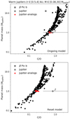 |
Fig. 5 Resulting C/O for our population of planets as a function of mass (black points). We note the Jupiter analogues from our population in red and observational data in grey. The data point for β Pic comes from GRAVITY Collaboration (2020) and the data for Jupiter from Asplund et al. (2009) and Li et al. (2020). The grey line accompanying Jupiter’s C/O (noted with |

4.3 C/O of warm Jupiters and Jupiter analogues
In Fig. 5, we show the resulting C/O for our population of warm Jupiters; the Jupiter analogues are highlighted with orange points. The main difference in the resulting atmospheric C/O between the reset and ongoing carbon erosion models is a horizontal shift in the C/O for the majority of planets (although not all, as explored below). The ongoing model, with its constant production of excess carbon, results in more carbon-rich planets compared to the reset model. There is a small discrepancy in this observation for a few planets that do not migrate past the erosion front (at 5 AU) until after they have accreted themajority of their atmosphere. These planets are difficult to see here but are highlighted and discussed in the following section.
We include an estimated C/O for Jupiter based on the measurements outlined in Asplund et al. (2009) and the recent oxygen measurement in Li et al. (2020). The error bars on this measurement are computed with the maximum and minimum C/Hs and O/Hs provided by the 1σ uncertainty in the above papers. Clearly, there is a wide range of possible C/Os based on these uncertain measurements. Including these uncertainties, Jupiter is most consistent with the Jupiter analogues in the ongoing carbon erosion model. This suggests that: Jupiter accretes the majority of its gas inside the carbon erosion front (inwards from its current orbit); and that there was an ongoing chemical process responsible for the processing of carbon from dust grains throughout the life of the solar nebula. This conclusion would hold if only carbon and oxygen were considered. New information regarding nitrogen and the noble gasses, however, suggests that Jupiter’s initial growth (and at least a fraction of its gas accretion) occurred outside the N2 ice line – at tens of AU (Bosman et al. 2019; Öberg & Wordsworth 2019). As is discussed in more detail below, there is a clear discrepancy between Jupiter’s C, N, and O elemental abundances when they are combined in comparison with the presented population of warm Jupiters.
In addition to Jupiter, we included the recent measurement of β Pic b made by GRAVITY Collaboration (2020). A ~ 12 MJupiter planet, β Pic b orbits at nearly 10 AU around its host star. Its C/O was determined from a pair of retrieval models based on interferometric observations of its atmosphere by GRAVITY Collaboration (2020). Given its orbital radius, it lies on the outer edge of what we defined as warm Jupiters. Indeed, planetesimal accretion models in general, and our formation models in particular, struggle to make large planets at these larger radii – and a formation scheme like pebble accretion (Ormel & Klahr 2010; Johansen et al. 2007; Bitsch et al. 2015) may be better suited to explain their existence. Regardless, we find that its measured C/O is consistent with planets that formed in the reset carbon refractory erosion model. This fact supports the idea that its formation occurred in a region of the disk outside both the water ice line and the refractory carbon erosion front. A more detailed discussion of the carbon erosion front is provided in Sect. 6.2. Outside the carbon erosion front, the gas is less carbon-rich than it could be inside the front, but the solids are more carbon-rich (recall Fig. 2, right panel).
4.4 The C/O main sequence and mass-metallicity relation
As in Paper I, we wish to understand the cause of the structure we see in Fig. 5. One major conclusion from Paper I was the C/O main sequence, which shows a tight inverse correlation between the fraction of the total mass made up of solids with the atmospheric C/O.
In Fig. 6, we show the same main sequence as presented in Paper I, with the data from Paper I included as faded points. As was done in Paper I, we differentiate between different planet masses; the mass bins are: low mass (M < 10 M⊕), Neptune-like (10 M⊕ < M < 40 M⊕), Saturn-like (40 M⊕ < M < 200 M⊕), Jupiter-like (200 M⊕ < M < 790 M⊕), and super-Jupiter (790 M⊕ < M). We find that the population of warm Jupiters tends to follow the main sequence up to a high C/O, where it then falls away from the trend. The high C/O end is dominated by the most massive planets (super-Jupiters), which have masses even higher than those obtained in Paper I. For these most-massive planets, their atmospheric chemistry is determined almost entirely by gas accretion (with solid accretion contributing less than 1%). As such, in the reset model (bottom panel), one group of the massive planets tends towards the C/O of the disk volatiles used in the chemistry calculation (vertical dashed line), while the other tends to higher C/Os. This trend is linked to where the planets accreted their gas: Inside the water ice line, the C/O tends to the disk C/O, while outside the water ice line the C/O tends to unity. These groupings are not discrete, however, and there are planets that seem to exist between the two extremes. We explore these groupings in more detail in Sect. 6.1. The same structure can be seen for the ongoing model (top panel), but it is shifted to higher C/Os due to the excess carbon that remains in the gas for the whole lifetime of the disk.
In Fig. 7, we present the mass-metallicity relation for the population of warm Jupiters and compare them directly to the population of hot Jupiters from Paper I. We find that (as in Paper I), the mass-metallicity relation directly follows from the main sequence – that is, the atmosphere metallicity falls with increasing planet mass. There is, in addition, a similar turn-off of the main trend at the higher-mass end, with massive planets (of at least a few Jupiter masses) tending towards a metallicity of 0.4–0.5 × solar. The low-mass end of the population aligns very closely with a region of O/H – mass parameter space that we attribute to planets having accreted their gas outside the water ice line (in an oxygen-poor region of the gas disk). In general, most of the lower-mass warm Jupiters sit lower than planets of similar masses in the hot Jupiter population, suggesting that this is a general trend. This is a reflection of the fact that warm Saturn and Neptune planets largely accreted their gas outside the water ice line. We explore further causes of the scatter seen here in a later section.
 |
Fig. 6 C/O main sequence for both the ongoing and reset carbon erosion models. The vertical dashed lines show the C/O = 0.4 that initialized the chemical model for the volatile component of the disk. The data from Paper I are also included as faded points to show that the population of warm Jupiters does indeed follow the general trend of the main sequence from Paper I. At the very high C/O end, the population appears to drop away from the trend found at lower C/Os. The planets in this part of the figure have very large masses and are dominated by gas accretion. The colour of each point denotes the trap from which the planet originated: ice line (blue), dead zone (orange), and heat transition (green). |
 |
Fig. 7 Mass-metallicity relation for the Alessi et al. (2020, APC) population of warm Jupiters, compared to the hot Jupiter population from Paper I (faded points). The Solar System giants (inferred by methane abundance and taken from Kreidberg et al. 2014), WASP-43 b (Kreidberg et al. 2014), GJ 436 b (Morley et al. 2017), and HAT-P-26 b (MacDonald & Madhusudhan 2019) (inferred from their water abundance) are also shown. In addition, we include the recent O/H measurement for Jupiter by Li et al. (2020) to show that, within uncertainty, the relation is independent of whether we used C/H or O/H to determine the metallicity. We include the O/Hs for our synthetic population and find that they follow the relation up to a mass of a few Jupiter masses, where they appear to flatten out. The colour of each point denotes the trap from which the planet originated: ice line (blue), dead zone (orange), and heat transition (green). This is a recreation of Fig. 12a from Paper I. |
5 Results: exploring different elemental ratios
While the C/O gives an important view of planet formation, it is not the only elemental ratio that can shed light on the problem. After carbon and oxygen, nitrogen is the next most abundant element in the Solar System. As discussed in Bosman et al. (2019), nitrogen chemistry is generally very simple since the majority of the element remains in its molecular form N2 at gas temperatures lower than ~500 K, while NH3 becomes dominant at higher temperatures (see Fig. A.1). Apart from this transition, there is the small build-up of HCN that was previously mentioned, which can hold of the order of 1% of the total nitrogen. We recall that we attribute this HCN enhancement to the carbon-rich region just below region C in Fig. 2.
In Fig. 8, we explore the role that nitrogen can play in understanding the physics of planet formation. Here, we plot the nitrogen-to-oxygen ratio (N/O) against the C/O for our population of warm Jupiters and for both the reset (square) and ongoing (circle) models. We note that since we run the reset and ongoing models separately for each planet formed in our model, each planet has two points on this figure – one for each carbon erosion model. We immediately see that the majority of planets fall on two straight lines – one for each of the carbon erosion models. Given that the slope of these lines is the nitrogen-to-carbon ratio (N/C), we can say that, for the planets in our model, the N/C is effectively constant. There are a number of planets, however, that do not conform to this rule; they can be grouped into carbon-rich planets in the reset model and carbon-poor planets in the ongoing model.
We include Jupiter in Fig. 8, using the elemental abundances reported in Asplund et al. (2009) and the new oxygen abundance from Li et al. (2020). While it seemed to be consistent with our population of Jupiter analogues accreting from the ongoing model in Fig. 5, Jupiter does not fit well into their C/O versus N/O parameter space. Within uncertainty, Jupiter’s C/O and N/O are consistent with the set of planets forming under the reset carbon erosion model. The inconsistency between its fit in the mass-C/O parameter space (more consistent with the ongoing model) and its fit here (with the reset model)suggest that its formation is inconsistent with the formation of warm Jupiters through the planetesimal formation presented here.
This inconsistency provides further evidence that Jupiter formed farther outwards in the disk than is achieved by our model, adding weight to a growing belief initially proposed in Öberg & Wordsworth (2019) and Bosman et al. (2019). They place Jupiter’s initial formation location outside the N2 ice line at tens of AU from the Sun and posit that Jupiter likely formed through the accretion of icy pebbles. Here we note that while the planets in our population typically acquire most of their carbon from gas sources, Bosman et al. (2019) propose that Jupiter’s carbon content is largely accreted from the frozen CO accompanying the accreting pebbles.
We now return to our population of planets. To quantify the distance away from the general trend of a constant N/C (as shown in in Fig. 8), we computed the deviation from the general trend for all planets in both erosion models relative to their N/O. To do this, we first computed a median N/C (N/Cmedian) for each of the ongoing and reset model results. We then assumed that the connection between N/Os and C/Os can be explained simply by a linear function with a slope equal to N/Cmedian. Deviation from this general trend would have the form:
 (7)
(7)
where N/O and C/O are the elemental ratios computed by our model. The absolute value of ΔN/C and its sign show how far it is from the line with slope N/Cmedian and in whatdirection.
We show the result of this calculation in Fig. 9. The majority of the points lie within 0.01 of ΔN/C = 0, meaning that their computed elemental abundances are consistent with the average planet in our population. There are a few planets that show larger deviations in Figs. 8 and 9, and we select three of these planets to investigate further. Planet A lies to the left of the average planet in the ongoing model. Its elemental abundances do not appear to depend on the erosion model in which it forms (its points overlap in Fig. 8). Planet B similarly sits far to the left of the average planet forming in the ongoing model. Finally, Planet C is a planet that lies far to the right of an average planet from the reset model. It shows C/O and N/O ratios that are similar to those of the previous two planets when it is formed in both the reset and ongoing carbon erosion models.
In Figs. 10a–c, we compare the radial evolution for each of these planets with the underlying gas C/O. To reflect the time frame that is most important for setting the chemical composition of each of their atmospheres, we only show contours up to the time where the planets’ growth is truncated in our planet formation model. Figures 10a and b show very similar pictures for Planets A and B. They each began growing out past the carbon erosion front (at 5 AU) and do not cross the front until after gas accretion has been terminated. As such, they have both predominately fed on more oxygen-poor (0.8 < C/O < 1) gas and slightly more oxygen-rich (0.6 < C/O < 0.8) solids.
While the two planets accrete nearly the same amount of solids in total (~ 9 M⊕), the main difference between them is that Planet B ends up accreting roughly an order of magnitude more gas than Planet A. This difference comes from the randomly generated maximum mass parameter from the population synthesis model, with Planet B being allowed to accrete for longer than Planet A. As such, Planet B accreted more gas, which leads to the chemistry in its atmosphere being more dependent on gas accretion than that of Planet A. A combined measurement of the C/Os and N/Os can help us understand the formation history of a planet and/or whether its natal disk underwent a refractory carbon erosion-like process.
In Fig. 10c, we compare the gas chemistry and orbital migration history for Planet C. We can see two important features in both the chemical composition of Planet C’s disk and the migration of the planet. The marginally carbon-rich region of the disk (below region C in Fig. 2) extends for much longer in time in this disk than in the disk shown in Fig. 2. The water ice line is also closer to the host star than in Fig. 2, which is a property of colder, less massive disks. Planet C begins its formation inside the carbon erosion front and coincidentally evolves inwards at the same rate (and at the same disk radius) as the erosion front in the reset model between ~ 0.5 and 0.65 Myr.
Because of Planet C’s orbital coincidence with the carbon erosion front, it spends a large portion of its formation accreting carbon-rich gas, even in the reset model; as such, it ends its formation with a very large C/O for its N/O. In addition, we find that Planet C’s C/O is nearly independent of the carbon erosion model because it spends a sufficiently long time accreting carbon-rich gas in the reset model. The difference in the C/Os of the two carbon erosion models for Planet C is only about 20% – much smaller than for a typical planet in our population.
 |
Fig. 8 Cross reference of the C/O with N/O for the population of warm Jupiters. We show here both the reset (squares) and ongoing (circles) models, which generally lie on a pair of straight lines. The slopes of these lines represent the elemental ratio N/C, which must be generally constant for most planets. The black point and error bars denote Jupiter’s C/O and N/O along with estimates for possible ranges. Due to the uncertainty in observed elemental abundances, Jupiter is consistentwith planets from the reset model but not with the ongoing model. The colour of each point denotes the trap from which the planet originated: ice line (blue), dead zone (orange), and heat transition (green). |
 |
Fig. 9 Deviation of N/O from the straight lines shown in Fig. 8, which represent a constant N/C across all planets in the population. For further analysis, we label three planets that show the wide deviation from the median N/C of the population. |
6 Discussion: What sets C/Os in warm-Jupiter atmospheres?
So far, we have reported on our findings for the C/Os and N/Os for either the entire population of warm Jupiters, or on an individual level. Generally, we find (as was the case in Paper I) that the fraction of mass that is accreted as solids into the atmosphere tends to heavily constrain the chemical properties that result. There are some exceptions, however, where the formation history – particularly the migration history – also has a noticeable impact on the resulting chemical properties of the atmosphere. In this section, we divide the population of planets by their initial disk conditions and study the resulting C/Os in the context of the environments in which they form.
6.1 Breakdown of C/Os by proto-planetary disk properties
In Fig. 11, we split the C/O results of both the ongoing and reset models into groups of disk metallicity, initial disk mass, and occupying planet trap. These groups are denoted by separate panels, marker shapes, and colours, respectively. The left-hand panel of the figure denotes the metal-poor systems ([Fe/H] ≤ −0.1), the middle panel denotes solar-like metallicities (− 0.1 < [Fe/H] ≤ 0.1), and the right-hand panel denotes metal-rich systems (0.1 < [Fe/H] ≤ 0.6). In each panel, we use dashed lines to differentiate between the atmospheric results for planets forming in the reset and ongoing models.
In Fig. 11, we bin the ongoing and reset model C/O data as discussed above. In the metal-poor and solar-like panels, the planets lie tightly correlated over a wide range of masses and C/Os. The tight correlation implies that disks with metal-poor and solar-like metallicities are the systems that most consistently produce planets that agree with the main sequence of the mass-C/O introduced in Paper I.
Generally speaking, planets trapped at the dead zone edge and in heat transition traps require the largest and lightest disk masses, respectively, to form warm Jupiters in our formation model. This is due to the timescale related to the initial core build-up, which needs to be sufficiently fast to build giant planets within the lifetime of the disk. The low-mass disks tend to be cooler, which moves the heat transition inwards to smaller radii and results in higher densities relative to what would be present in higher-mass disks. Conversely, the dead zone trap is best at building planets in disks with higher initial masses. Thedead zone edge is computed semi-analytically in Alessi et al. (2020) and is less sensitive to the initial disk mass, as is the heat transition; therefore, higher disk masses lead to higher densities at the trap and lead to faster core growth. For lower-mass disks at these metallicities, dead-zone-trapped planets lead more often to hot Jupiters.
The metal-rich panel of planets is the first to show significant deviations from the general trends of the two other panels. As already discussed in relation to Fig. 6, a second group of warm Jupiters have higher C/Os than what would be predicted from their planet masses or from the fraction of mass they have accreted as solids. This group is more evenly spread when binning by metallicity than was suggested in Fig. 6, showing that the metal-rich systems lead to higher chemical diversity than the lower-metallicity systems. Given their high C/Os, the most likely scenario for these planets is that they accreted the majority of their gas outside the water ice line. This is most easily done in the metal-rich disks because there is a higher density of solids (by construction) when the metallicity is higher, which reduces the timescale related to the initial core growth. In these systems, core formation can occur efficiently farther away from the host star than in the lower-metallicity systems. This generates a wider variety of chemical properties as the planets sample chemically different regions of the disk. This variety causes some of the scatter seen in Fig. 7 because the planets’ O/H metallicity is constrained by the accretion of gas that is generally more oxygen-poor outside the water ice line.
We also show the reset model in Fig. 11. Generally, the difference between the two sides of the panels is a shift of all points to less carbon-rich atmospheres in the reset model, with the exception of a few particular planets (three of which were discussed above). In particular, the heat transition planet in the left panel stands out as having the highest C/O in that group (this was Planet C from above), and the dead zone planet with M ~ MJupiter in the right panel that lies on the dashed line (this was Planet A from above). Otherwise, the structure of the metal-poor and solar-like groups of planets are grouped by planet masses and C/Os, similar to what was done for the ongoing model.
In the metal-rich panel, we see a slight change in the structure of the distribution of planets. The dead-zone-trapped planets tend to be more carbon-rich than the planets coming from the water ice line trap in the reset model. As previously argued, the planets forming at the dead zone edge tend to start their evolution farther from the host star than the water ice line planets. As such, they accrete gas that is more carbon-rich than planets inside the water ice line. In the reset model, the excess carbon is lost to the host star after less than 0.8 Myr, and planets forming farther outwards in the disk are more sensitive to the volatile chemistry than in the ongoing model.
Overall, we find that for solar-like and metal-poor disks, there is a reasonably tight correlation between the planet mass and the C/O. This implies that the main sequence derived from the population of hot Jupiters extends easily to the warm Jupiters, with much of the scatter at the high planet mass end being produced by metal-rich systems. These metal-rich systems were not found in Paper I because high-metallicity disks tend to build warm Jupiters over hot Jupiters in our formation model. At the low planet mass end of the distribution, there appears to be a small deviation in the C/Os caused by differences in initial disk masses. This is particularly apparent in the solar-like metallicity systems, where we see that planets generated in low-mass disks tend to be less carbon-rich than planets of the same planet mass formed from high-mass disks.
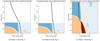 |
Fig. 10 Comparison between the locations (black line) and the underlying chemical properties of the gas (coloured contours) ofPlanets A, B, and C. We note that we only show the C/O up to the point where gas accretion is shut off in our formation model since the disk no longer impacts the atmosphere once accretion is stopped. The contours are the same as in Fig. 2. We note the change in the time axis in the third panel. |
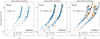 |
Fig. 11 C/Os for synthetic planets in both of the ongoing and reset carbon erosion models. The data for each erosion model are separated on each panel by a dashed line. Each panel separates the planets by the proto-planetary disk metallicity. Left-hand panel: low metallicity, middle panel: solar-like metallicity (− 0.1 < [Fe/H] ≤ 0.1), and right-hand panel: high metallicity (0.1 < [Fe/H] ≤ 0.6). The different point shapes represent different initial disk masses. The colour of each point denotes the trap from which the planet originated: ice line (blue), dead zone (orange), and heat transition (green). Generally, there is a shift in the C/Os between planets growing in the reset and ongoing carbon erosion models. However, there are some exceptions: for example, the heat transition planet (green point) in the first panel has nearly the same C/O in both the reset and ongoing models (this is Planet C from above). |
6.2 Impact of shifting the carbon erosion front
For the majority of the paper, and the entirety of Paper I, we have assumed that the process of carbon erosion began at 5 AU with the excess carbon smoothly increasing to 1 AU, after which we maintained a constant carbon excess. This assumption, however, is largely based on current observations of the refractory component of carbon in the Earth’s mantle, asteroids, comets, and Jupiter’s current orbital radius (Bergin et al. 2015; Mordasini et al. 2016). Jupiter very likely migrated to its current location, either from smaller radii during a Grand Tack or from larger radii. Indeed, Jupiter’s migration is required to explain the current population of Trojan asteroids (Pirani et al. 2019).
Since the chemical process that drives refractory erosion is still an open question, and Jupiter very likely (must have)migrated during its formation, it is completely reasonable to vary the radial location of the carbon erosion front. For simplicity, we anchored the inner region of the function that describes the carbon erosion such that the excess carbon is always constant under 1 AU. We then varied the carbon erosion front between 3 and 7 AU. This radius range ensures that the shifting erosion front remains relevant for the presented population of planets.
The location of the erosion front impacts the chemical properties of the disk in two ways. First, it changes the partitioning of the excess carbon between the gas and refractories through the location where carbon is removed from the grains. Moving the front inwards implies that there is generally less carbon available in the gas for accretion; it also implies a wider range of radii where the refractories remain carbon-rich. In the reset model, the second effect is the timing at which the excess carbon is lost to the host star. We keep the advection speed the same throughout this work, so moving the front inwards shortens the time it takes the excess carbon to accrete into the host star. The opposite is true if we move the erosion radius farther away from the host star.
In Fig. 12, for illustrative purposes, we show a comparison between a few of our planet tracks (which describe the planet’s evolution through the mass-semi-major axis diagram), the carbon erosion front, and the resulting excess carbon generated from the refractories (contours). We show the distribution of the excess carbon in the ongoing model for an erosion front of 5 AU (fiducial model). Clearly, if the front were shifted inwards, then the excess carbon available to some planets would be reduced; if it were moved outwards, then a higher carbon excess would be available to some of the growing planets earlier in their formation.
In Fig. 13, we show the impact of shifting the carbon erosion front between 3 and 7 AU for both the ongoing (top panel) and reset (bottom panel) models. The planets forming in the ongoing model show two distinct shifts in relation to the change in the carbon erosion front. Lower-mass planets (M ≲ 0.55 MJupiter) shift to higher C/Os when the carbon erosion front is shifted to smaller radii, while the opposite is true for higher-mass planets. This difference highlights how higher-mass planets depend more on gas accretion for setting their chemical composition, while lower-mass planets are more dependent on solid accretion. In a sense, a better classification of “ice giants” would be planets with M ≲ 0.55 MJupiter ~ 175 M⊕, and of gas giants as planet with M > 175 M⊕. Although we admit that such a classification would be confusing as it would change our Solar System to contain one gas giant and three ice giants, such a classification would nevertheless better capture the physics and chemistry of planet formation.
In the bottom panel of Fig. 13, we see that the majority of the planets are shifted to more carbon-rich atmosphereswhen the carbon erosion front is moved inwards. This is because there is more total carbon available for planetary accretion in the reset model since fewer solids are chemically processed and less carbon is lost to the host star. The lower-mass planets see the highest shift since their chemical composition is most dependent on the refractory source of carbon. There are a few planets where the opposite trend is observed, with higher C/Os when the carbon erosion front is farther away from the host star. Like Planet C from earlier, this is due to a coincidence between the excess carbon in the gas and the period of rapid gas accretion during the planets’ formation.
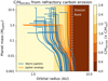 |
Fig. 12 Some selected planetary tracks compared to the location of the erosion front, and the resulting distribution of excess carbon (in contours). |
7 Conclusion
We have presented a population of warm Jupiters derived from a full planet population synthesis model starting from planetesimal accretion. We computed the chemical evolution of the disk volatiles in each of the disks used for the population synthesis calculation to predict the carbon, oxygen, and nitrogen abundances in the gas and ice. When combined with a model for the refractory chemistry – particularly the carbon – we computed the evolution of the total carbon, oxygen, and nitrogen content of each proto-planetary disk. These calculations are combined with the planet tracks derived from the formation model to predict the resulting C/Os and N/Os in the planetary atmospheres.
We generally find that:
-
like the hot Jupiters in Paper I (Cridland et al. 2019b), there is a reasonably tight correlation between the C/O in the atmosphere and the planetary mass;
-
the spread in the aforementioned correlation is linked to planets forming in metal-rich disks, which are capable of producing more chemically varied atmospheres due to a more rapid initial core build-up;
-
the main sequence of the C/O versus fraction of solid mass accreted into the atmosphere reported in Paper I is upheld for the warm Jupiters. High-mass planets tend to curve away from the general trend, moving asymptotically towards the disk volatile C/O in the case of the reset model, and to C/O ~ 1 for the ongoing model;
-
there is an arm of higher C/Os caused by the metal-rich disks seen in the main sequence that asymptote to a higher C/O in both carbon erosion models;
-
including N/Os in our analysis weakens the viability of planetesimal formation in the inner disk as the formation mechanism of Jupiter. This result agrees with the purely chemical analyses of Öberg & Wordsworth (2019) and Bosman et al. (2019), which place Jupiter’s formation origin outside tens of AU;
-
combining C/Os and N/Os additionally allows us to identify planets that exclusively accrete their atmosphere outside of the refractory carbon erosion front – a rare situation for this population of planets;
-
shifting the carbon erosion front shows the importance of solid accretion in determining the chemical structure of planetary atmospheres, particularly for planets with masses ≲175 M⊕.
The observability of these types of planets will continue to be a challenge as they lie in a range of orbital periods that makes their chemical characterization difficult by both transit spectroscopy and direct imaging. There is a single exoplanet, WASP-167e, that has had its orbital period (of 1071 days) characterized by both Kepler and Spitzer with enough accuracy to justify an attempt at transit spectroscopy with JWST (Dalba & Tamburo 2019). As we enter into the next generation of Extremely Large Telescopes, and with improvements to coronagraphy that are ongoing, it is possible that a direct emission spectrum of warm Jupiters could be taken. This could unlock a whole new range of planets to study chemically.
Along with the observational challenges, there is more to be done on the modelling side of planet formation and astrochemistry. This work has made strides to include a simple model that describes the chemical properties of the refractories in the proto-planetary disks. The physics that describe how this material finds its way into the atmosphere of the planet, and where the carbon and oxygen are deposited in the atmosphere, still remain complicated problems that are beyond the scope of this paper. The strict atmospheric mass cutoff that governs the delivery of refractory material into the atmosphere is simply implemented in our model (as described in Paper I). Self-consistently computing the arrival and destruction of planetesimals in the atmosphere of a giant planet could deliver refractory material that is so deep in the atmosphere that it is unable to impact the observable C/Os. Such a complication is currently also beyond the scope of this work.
Furthermore, the proto-planetary disk models that are used in our planet formation models are smooth – representing a much simpler picture than is being seen in current high resolution surveys of young star forming regions. These surveys also push the start time for planet formation – or at least the formation of the first planetesimals – farther back into the Class 0 or Class I young stellar systems (Tychoniec et al. 2018). It is perfectly possible that by the time a Class II disk (classically called a proto-planetary disk as it was believed to be the natal system for planets) emerges from the envelope of the proto-star, planets will have already almost fully formed. Indeed, the marginally Class I/II system HL Tau already shows wide shallow gaps that are often attributed to the presence of at least one large planet (ALMA Partnership 2015; Tamayo et al. 2015). If it is indeed true that the majority of initial core growth and atmosphere accretion (important for determining the chemistry of the atmosphere) occurs in the Class 0/I phase, then we will need adjust our disk models to incorporate the properties of these systems.
With all that being said, it is safe to say that there is still much that can be learned about the physical processes governing planet formation from models such as the ones presented here. Over the next few decades as we begin to chemically characterize the atmospheres of planets, which are now easy to find, we should see another surge in our understanding of planet formation. Such a surge, possibly driven by JWST or through the upcoming European Space Agency’s ARIEL mission, could rival the one we witnessed in the early years of the Kepler mission.
Acknowledgements
Astrochemistry in Leiden is supported by the European Union A-ERC grant 291141 CHEMPLAN, by the Netherlands Research School for Astronomy (NOVA). The work made use of the Shared Hierarchical Academic Research Computating Network (SHARCNET: www.sharcnet.ca) and Compute/Calcul Canada. A.J.C acknowledges additional support by the European Union ERC grant H2020 ExoplanetBio supervised by Ignas Snellen. R.E.P. is supported by an NSERC Discovery Grant. M.A. acknowledges funding from NSERC through the PGS-D Alexander Graham Bell scholarship.
Appendix A Breakdown of most abundant species
Here we show the most abundant species found in one particular chemical model in our population of disks. The carbon- and oxygen-carrying species are predominately H2O, OH, and CO. There are periods of time (and ranges of radii) where CO2 becomes abundant on the icy grains while molecular oxygen and atomic oxygen become abundant in the gas. Frozen OH is mainly made from the dissociation of frozen water by UV photons induced by collisions of cosmic rays with molecular hydrogen. A very small amount of carbon- and nitrogen-bearing species, such as CH4, HCN, and C6 H6, can be found in the gas phase; however, these species do not survive throughout the chemical evolution of the disk. Unlike some chemical models, ours does not produce large amounts of gaseous CO2 – which is generally produced through grain surface reactions that are not included in our model.
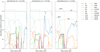 |
Fig. A.1 Abundances for the most abundant gas species in the chemical model. Annotated on the right-most panel are the most abundant species in our chemical model. |
References
- Alessi, M., & Pudritz, R. E. 2018, MNRAS, 478, 2599 [NASA ADS] [CrossRef] [Google Scholar]
- Alessi, M., Pudritz, R. E., & Cridland, A. J. 2017, MNRAS, 464, 428 [NASA ADS] [CrossRef] [Google Scholar]
- Alessi, M., Pudritz, R. E., & Cridland, A. J. 2020, MNRAS, 493, 1013 [CrossRef] [Google Scholar]
- Alibert, Y., Mousis, O., Mordasini, C., & Benz, W. 2005, ApJ, 626, L57 [NASA ADS] [CrossRef] [Google Scholar]
- ALMA Partnership (Brogan, C. L., et al.) 2015, ApJ, 808, L3 [NASA ADS] [CrossRef] [Google Scholar]
- Anderson, D. E., Bergin, E. A., Blake, G. A., et al. 2017, ApJ, 845, 13 [NASA ADS] [CrossRef] [Google Scholar]
- Ansdell, M., Williams, J. P., van der Marel, N., et al. 2016, ApJ, 828, 46 [Google Scholar]
- Asplund, M., Grevesse, N., Sauval, A. J., & Scott, P. 2009, ARA&A, 47, 481 [NASA ADS] [CrossRef] [Google Scholar]
- Aumann, H. H., Gillespie, C. M., J., & Low, F. J. 1969, ApJ, 157, L69 [NASA ADS] [CrossRef] [Google Scholar]
- Bergin, E. A., Blake, G. A., Ciesla, F., Hirschmann, M. M., & Li, J. 2015, Proc. Natl. Acad. Sci., 112, 8965 [NASA ADS] [CrossRef] [Google Scholar]
- Birnstiel, T., Klahr, H., & Ercolano, B. 2012, A&A, 539, A148 [NASA ADS] [CrossRef] [EDP Sciences] [Google Scholar]
- Bitsch, B., Lambrechts, M., & Johansen, A. 2015, A&A, 582, A112 [NASA ADS] [CrossRef] [EDP Sciences] [Google Scholar]
- Bosman, A. D., Walsh, C., & van Dishoeck, E. F. 2018, A&A, 618, A182 [NASA ADS] [CrossRef] [EDP Sciences] [Google Scholar]
- Bosman, A. D., Cridland, A. J., & Miguel, Y. 2019, A&A, 632, L11 [CrossRef] [EDP Sciences] [Google Scholar]
- Brewer, J. M., & Fischer, D. A. 2016, ApJ, 831, 20 [NASA ADS] [CrossRef] [Google Scholar]
- Brogi, M., de Kok, R. J., Birkby, J. L., Schwarz, H., & Snellen, I. A. G. 2014, A&A, 565, A124 [NASA ADS] [CrossRef] [EDP Sciences] [Google Scholar]
- Chambers, J. E. 2009, ApJ, 705, 1206 [NASA ADS] [CrossRef] [Google Scholar]
- Chambers, J. 2018, ApJ, 865, 30 [NASA ADS] [CrossRef] [Google Scholar]
- Chametla, R. O., D’Angelo, G., Reyes-Ruiz, M., & Sánchez-Salcedo, F. J. 2020, MNRAS, 492, 6007 [CrossRef] [Google Scholar]
- Cleeves, L. I., Bergin, E. A., & Adams, F. C. 2014, ApJ, 794, 123 [NASA ADS] [CrossRef] [Google Scholar]
- Crida, A. 2009, ApJ, 698, 606 [NASA ADS] [CrossRef] [Google Scholar]
- Cridland, A. J. 2018, A&A, 619, A165 [NASA ADS] [CrossRef] [EDP Sciences] [Google Scholar]
- Cridland, A. J., Pudritz, R. E., & Alessi, M. 2016, MNRAS, 461, 3274 [Google Scholar]
- Cridland, A. J., Pudritz, R. E., Birnstiel, T., Cleeves, L. I., & Bergin, E. A. 2017a, MNRAS, 469, 3910 [NASA ADS] [CrossRef] [Google Scholar]
- Cridland, A. J., Pudritz, R. E., & Birnstiel, T. 2017b, MNRAS, 465, 3865 [NASA ADS] [CrossRef] [Google Scholar]
- Cridland, A. J., Eistrup, C., & van Dishoeck, E. F. 2019a, A&A, 627, A127 [NASA ADS] [CrossRef] [EDP Sciences] [Google Scholar]
- Cridland, A. J., van Dishoeck, E. F., Alessi, M., & Pudritz, R. E. 2019b, A&A, 632, A63 [NASA ADS] [CrossRef] [EDP Sciences] [Google Scholar]
- Cridland, A. J., Pudritz, R. E., & Alessi, M. 2019c, MNRAS, 484, 345 [NASA ADS] [CrossRef] [Google Scholar]
- Cridland, A. J., Bosman, A. D., & van Dishoeck, E. F. 2020, A&A, 635, A68 [CrossRef] [EDP Sciences] [Google Scholar]
- Dalba, P. A., & Tamburo, P. 2019, ApJ, 873, L17 [CrossRef] [Google Scholar]
- D’Angelo, G., Durisen, R. H., & Lissauer, J. J. 2010, Exoplanet, ed. S. Seager (Tucson, AZ: University of Arizona Press), 319 [Google Scholar]
- Dodson-Robinson, S. E., Veras, D., Ford, E. B., & Beichman, C. A. 2009, ApJ, 707, 79 [NASA ADS] [CrossRef] [Google Scholar]
- Dra̧żkowska, J., & Alibert, Y. 2017, A&A, 608, A92 [NASA ADS] [CrossRef] [EDP Sciences] [Google Scholar]
- Eistrup, C., Walsh, C., & van Dishoeck, E. F. 2016, A&A, 595, A83 [NASA ADS] [CrossRef] [EDP Sciences] [Google Scholar]
- Eistrup, C., Walsh, C., & van Dishoeck, E. F. 2018, A&A, 613, A14 [NASA ADS] [CrossRef] [EDP Sciences] [Google Scholar]
- Fogel, J. K. J., Bethell, T. J., Bergin, E. A., Calvet, N., & Semenov, D. 2011, ApJ, 726, 29 [NASA ADS] [CrossRef] [Google Scholar]
- Gandhi, S., & Madhusudhan, N. 2018, MNRAS, 474, 271 [Google Scholar]
- GRAVITY Collaboration (Lacour, S., et al.) 2019, A&A, 623, L11 [NASA ADS] [CrossRef] [EDP Sciences] [Google Scholar]
- GRAVITY Collaboration (Nowak, M., et al.) 2020, A&A, 633, A110 [NASA ADS] [CrossRef] [EDP Sciences] [Google Scholar]
- Hasegawa, Y., & Pudritz, R. E. 2010, ApJ, 710, L167 [NASA ADS] [CrossRef] [Google Scholar]
- Hasegawa, Y., & Pudritz, R. E. 2011, MNRAS, 417, 1236 [NASA ADS] [CrossRef] [Google Scholar]
- Hasegawa, Y., & Pudritz, R. E. 2013, ApJ, 778, 78 [NASA ADS] [CrossRef] [Google Scholar]
- Helled, R., Bodenheimer, P., Podolak, M., et al. 2014, in Protostars and Planets VI, eds. H. Beuther, R. S. Klessen, C. P. Dullemond, & T. Henning (Tucson, AZ: University of Arizona Press), 643 [Google Scholar]
- Helling, C., Woitke, P., Rimmer, P. B., et al. 2014, Life, 4, 142 [NASA ADS] [CrossRef] [Google Scholar]
- Ida, S., & Lin,D. N. C. 2004, ApJ, 604, 388 [Google Scholar]
- Ikoma, M., Nakazawa, K., & Emori, H. 2000, ApJ, 537, 1013 [NASA ADS] [CrossRef] [Google Scholar]
- Johansen, A., Oishi, J. S., Mac Low, M.-M., et al. 2007, Nature, 448, 1022 [Google Scholar]
- Klarmann, L., Ormel, C. W., & Dominik, C. 2018, A&A 618, L1 [NASA ADS] [CrossRef] [EDP Sciences] [Google Scholar]
- Kokubo, E., & Ida, S. 2002, ApJ, 581, 666 [Google Scholar]
- Kreidberg, L., Bean, J. L., Désert, J.-M., et al. 2014, ApJ, 793, L27 [NASA ADS] [CrossRef] [Google Scholar]
- Krijt, S., Bosman, A. D., Zhang, K., et al. 2020, ApJ, 899, 134 [CrossRef] [Google Scholar]
- Lambrechts, M., & Johansen, A. 2014, A&A, 572, A107 [NASA ADS] [CrossRef] [EDP Sciences] [Google Scholar]
- Lee, J.-E., Bergin, E. A., & Nomura, H. 2010, ApJ, 710, L21 [NASA ADS] [CrossRef] [Google Scholar]
- Li, C., Ingersoll, A., Bolton, S., et al. 2020, Nat. Astron., 4, 609 [CrossRef] [Google Scholar]
- Lin, D. N. C., & Papaloizou, J. 1986, ApJ, 309, 846 [NASA ADS] [CrossRef] [Google Scholar]
- Line, M. R., Knutson, H., Wolf, A. S., & Yung, Y. L. 2014, ApJ, 783, 70 [Google Scholar]
- Lyra, W., Paardekooper, S.-J., & Mac Low, M.-M. 2010, ApJ, 715, L68 [NASA ADS] [CrossRef] [Google Scholar]
- MacDonald, R. J., & Madhusudhan, N. 2019, MNRAS, 486, 1292 [Google Scholar]
- Madhusudhan, N. 2012, ApJ, 758, 36 [NASA ADS] [CrossRef] [Google Scholar]
- Madhusudhan, N., Amin, M. A., & Kennedy, G. M. 2014, ApJ, 794, L12 [Google Scholar]
- Manara, C. F., Morbidelli, A., & Guillot, T. 2018, A&A, 618, L3 [NASA ADS] [CrossRef] [EDP Sciences] [Google Scholar]
- Masset, F. S., Morbidelli, A., Crida, A., & Ferreira, J. 2006, ApJ, 642, 478 [NASA ADS] [CrossRef] [Google Scholar]
- McNally, C. P., Nelson, R. P., & Paardekooper, S.-J. 2018, MNRAS, 477, 4596 [NASA ADS] [CrossRef] [Google Scholar]
- McNally, C. P., Nelson, R. P., Paardekooper, S.-J., Benítez-Llambay, P., & Gressel, O. 2020, MNRAS, 493, 4382 [CrossRef] [Google Scholar]
- Mordasini, C., Alibert, Y., Benz, W., & Naef, D. 2009, A&A, 501, 1161 [NASA ADS] [CrossRef] [EDP Sciences] [Google Scholar]
- Mordasini, C., Mollière, P., Dittkrist, K.-M., Jin, S., & Alibert, Y. 2015, Int. J. Astrobiol., 14, 201 [CrossRef] [Google Scholar]
- Mordasini, C., van Boekel, R., Mollière, P., Henning, T., & Benneke, B. 2016, ApJ, 832, 41 [NASA ADS] [CrossRef] [Google Scholar]
- Morley, C. V., Knutson, H., Line, M., et al. 2017, AJ, 153, 86 [NASA ADS] [CrossRef] [Google Scholar]
- Moses, J. I., Madhusudhan, N., Visscher, C., & Freedman, R. S. 2013, ApJ, 763, 25 [NASA ADS] [CrossRef] [Google Scholar]
- Öberg, K. I., & Wordsworth, R. 2019, AJ, 158, 194 [Google Scholar]
- Öberg, K. I., Murray-Clay, R., & Bergin, E. A. 2011, ApJ, 743, L16 [NASA ADS] [CrossRef] [Google Scholar]
- Ormel, C. W., & Klahr, H. H. 2010, A&A, 520, A43 [NASA ADS] [CrossRef] [EDP Sciences] [Google Scholar]
- Pinhas, A., Madhusudhan, N., Gandhi, S., & MacDonald, R. 2019, MNRAS, 482, 1485 [Google Scholar]
- Pinilla, P., Klarmann, L., Birnstiel, T., et al. 2016, A&A, 585, A35 [NASA ADS] [CrossRef] [EDP Sciences] [Google Scholar]
- Pirani, S., Johansen, A., Bitsch, B., Mustill, A. J., & Turrini, D. 2019, A&A, 623, A169 [NASA ADS] [CrossRef] [EDP Sciences] [Google Scholar]
- Pollack, J. B., Hubickyj, O., Bodenheimer, P., et al. 1996, Icarus, 124, 62 [NASA ADS] [CrossRef] [Google Scholar]
- Pontoppidan, K. M., Salyk, C., Bergin, E. A., et al. 2014, Protostars and Planets VI (Tucson, AZ: University of Arizona Press), 363 [Google Scholar]
- Raymond, S. N., & Morbidelli, A. 2014, IAU Symp., 310, 194 [NASA ADS] [CrossRef] [Google Scholar]
- Tamayo, D., Triaud, A. H. M. J., Menou, K., & Rein, H. 2015, ApJ, 805, 100 [NASA ADS] [CrossRef] [Google Scholar]
- Tychoniec, Ł., Tobin, J. J., Karska, A., et al. 2018, ApJS, 238, 19 [NASA ADS] [CrossRef] [Google Scholar]
- Tychoniec, Ł., Manara, C. F., Rosotti, G. P., et al. 2020, A&A, 640, A19 [CrossRef] [EDP Sciences] [Google Scholar]
- Voelkel, O., Klahr, H., Mordasini, C., Emsenhuber, A., & Lenz, C. 2020, A&A, 642, A75 [NASA ADS] [CrossRef] [EDP Sciences] [Google Scholar]
- Walsh, K. J., Morbidelli, A., Raymond, S. N., O’Brien, D. P., & Mandell, A. M. 2011, Nature, 475, 206 [NASA ADS] [CrossRef] [PubMed] [Google Scholar]
- Walsh, C., Nomura, H., & van Dishoeck, E. 2015, A&A, 582, A88 [NASA ADS] [CrossRef] [EDP Sciences] [Google Scholar]
- Ward, W. R. 1991, Lunar Planetary Science Conference, 22 [Google Scholar]
- Ward, W. R. 1997, ApJ, 482, L211 [NASA ADS] [CrossRef] [Google Scholar]
- Wei, C.-E., Nomura, H., Lee, J.-E., et al. 2019, ApJ, 870, 129 [NASA ADS] [CrossRef] [Google Scholar]
- Wittenmyer, R. A., Tinney, C. G., O’Toole, S. J., et al. 2011, ApJ, 727, 102 [NASA ADS] [CrossRef] [Google Scholar]
- Wright, J. T., Marcy, G. W., Howard, A. W., et al. 2012, ApJ, 753, 160 [NASA ADS] [CrossRef] [Google Scholar]
Extracted from exoplanet.eu.
In principle, the dust surface density also evolves due to the production of planetesimals (for example, see Voelkel et al. 2020); however, our current implementation is limited as it does not allow such a connection. In practice, such a connection leads to less efficient planetesimal formation and slower initial core growth. Overall, this change will not drastically change the main conclusions of the paper.
But see Alessi & Pudritz (2018) for the full details of the disk model.
Practically speaking, we increase τc,acc by two orders of magnitude in this stage.
We are using the typical notation where [Fe/H] ≡
 , such that [Fe/H]⊙ = 0.
We assume that the core does not contribute to the observed chemical composition of the atmosphere.
That is, the C/O of the envelope that has collected around the proto-planet.
All Figures
|
Fig. 1 Current population of confirmed exoplanets extracted on March 7, 2020 (from exoplanet.eu). We note the range of masses and semi-major axes that define our warm Jupiters with black lines. The majority of planets in this range were discovered through direct imaging, radial velocity, and microlensing. |
| In the text | |
|
Fig. 2 Evolution and radial distribution of the midplane C/O in the gas and solids in one of the disk models used for this work. Specifically, we show the chemistry of the disk in the reset scenario of refractory erosion, which governs the high C/O early on in the disk’s life (A). We similarly note the region of the disk with high and low water vapour abundances (B and D, respectively), the carbon-poor region due to refractory erosion (E), and a region where gaseous CO is converted to frozen CO2 (C). The more carbon-rich region (F) exists at larger radii than the carbon erosion front. Orange denotes carbon-rich regions (C/O > 1) while blue denotes carbon-poor regions (C/O < 1). The nominalvolatile C/O = 0.4 and the refractory C/O = 2. |
| In the text | |
|
Fig. 3 Typical evolution of the atmospheric C/O as a proto-planet grows (top panel). We show the results for each of the example planets for each of the ongoing (solid line) and reset (dashed line) carbon erosion models. In addition, we show the mass and orbital radius evolution of the same planets (bottom panel). |
| In the text | |
|
Fig. 4 Final mass and orbital range of synthetic planets from the Alessi et al. (2020, APC) population of planets. The colour coding here (and throughout) denotes the planet trap in which the planet initially grew. Generally, ice line planets (blue) start closer than the dead-zone (orange) and heat-transition (green) planets. The population of warm Jupiters exists predominately between 1 and 4 AU. |
| In the text | |
|
Fig. 5 Resulting C/O for our population of planets as a function of mass (black points). We note the Jupiter analogues from our population in red and observational data in grey. The data point for β Pic comes from GRAVITY Collaboration (2020) and the data for Jupiter from Asplund et al. (2009) and Li et al. (2020). The grey line accompanying Jupiter’s C/O (noted with |
| In the text | |
|
Fig. 6 C/O main sequence for both the ongoing and reset carbon erosion models. The vertical dashed lines show the C/O = 0.4 that initialized the chemical model for the volatile component of the disk. The data from Paper I are also included as faded points to show that the population of warm Jupiters does indeed follow the general trend of the main sequence from Paper I. At the very high C/O end, the population appears to drop away from the trend found at lower C/Os. The planets in this part of the figure have very large masses and are dominated by gas accretion. The colour of each point denotes the trap from which the planet originated: ice line (blue), dead zone (orange), and heat transition (green). |
| In the text | |
|
Fig. 7 Mass-metallicity relation for the Alessi et al. (2020, APC) population of warm Jupiters, compared to the hot Jupiter population from Paper I (faded points). The Solar System giants (inferred by methane abundance and taken from Kreidberg et al. 2014), WASP-43 b (Kreidberg et al. 2014), GJ 436 b (Morley et al. 2017), and HAT-P-26 b (MacDonald & Madhusudhan 2019) (inferred from their water abundance) are also shown. In addition, we include the recent O/H measurement for Jupiter by Li et al. (2020) to show that, within uncertainty, the relation is independent of whether we used C/H or O/H to determine the metallicity. We include the O/Hs for our synthetic population and find that they follow the relation up to a mass of a few Jupiter masses, where they appear to flatten out. The colour of each point denotes the trap from which the planet originated: ice line (blue), dead zone (orange), and heat transition (green). This is a recreation of Fig. 12a from Paper I. |
| In the text | |
|
Fig. 8 Cross reference of the C/O with N/O for the population of warm Jupiters. We show here both the reset (squares) and ongoing (circles) models, which generally lie on a pair of straight lines. The slopes of these lines represent the elemental ratio N/C, which must be generally constant for most planets. The black point and error bars denote Jupiter’s C/O and N/O along with estimates for possible ranges. Due to the uncertainty in observed elemental abundances, Jupiter is consistentwith planets from the reset model but not with the ongoing model. The colour of each point denotes the trap from which the planet originated: ice line (blue), dead zone (orange), and heat transition (green). |
| In the text | |
|
Fig. 9 Deviation of N/O from the straight lines shown in Fig. 8, which represent a constant N/C across all planets in the population. For further analysis, we label three planets that show the wide deviation from the median N/C of the population. |
| In the text | |
|
Fig. 10 Comparison between the locations (black line) and the underlying chemical properties of the gas (coloured contours) ofPlanets A, B, and C. We note that we only show the C/O up to the point where gas accretion is shut off in our formation model since the disk no longer impacts the atmosphere once accretion is stopped. The contours are the same as in Fig. 2. We note the change in the time axis in the third panel. |
| In the text | |
|
Fig. 11 C/Os for synthetic planets in both of the ongoing and reset carbon erosion models. The data for each erosion model are separated on each panel by a dashed line. Each panel separates the planets by the proto-planetary disk metallicity. Left-hand panel: low metallicity, middle panel: solar-like metallicity (− 0.1 < [Fe/H] ≤ 0.1), and right-hand panel: high metallicity (0.1 < [Fe/H] ≤ 0.6). The different point shapes represent different initial disk masses. The colour of each point denotes the trap from which the planet originated: ice line (blue), dead zone (orange), and heat transition (green). Generally, there is a shift in the C/Os between planets growing in the reset and ongoing carbon erosion models. However, there are some exceptions: for example, the heat transition planet (green point) in the first panel has nearly the same C/O in both the reset and ongoing models (this is Planet C from above). |
| In the text | |
|
Fig. 12 Some selected planetary tracks compared to the location of the erosion front, and the resulting distribution of excess carbon (in contours). |
| In the text | |
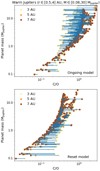 |
Fig. 13 Same as Fig. 5 but including the effect of shifting the erosion between 3 and 7 AU. |
| In the text | |
|
Fig. A.1 Abundances for the most abundant gas species in the chemical model. Annotated on the right-most panel are the most abundant species in our chemical model. |
| In the text | |
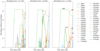 |
Fig. A.2 Same as Fig. A.1 but for the most abundant ice species. |
| In the text | |
Current usage metrics show cumulative count of Article Views (full-text article views including HTML views, PDF and ePub downloads, according to the available data) and Abstracts Views on Vision4Press platform.
Data correspond to usage on the plateform after 2015. The current usage metrics is available 48-96 hours after online publication and is updated daily on week days.
Initial download of the metrics may take a while.