| Issue |
A&A
Volume 642, October 2020
|
|
|---|---|---|
| Article Number | A34 | |
| Number of page(s) | 20 | |
| Section | Planets and planetary systems | |
| DOI | https://doi.org/10.1051/0004-6361/201936201 | |
| Published online | 02 October 2020 | |
Plasma and magnetic-field structures near the Martian induced magnetosphere boundary
I. Plasma depletion region and tangential discontinuity
1
State Key Laboratory of Lunar and Planetary Sciences, Macau University of Science and Technology,
Macao,
PR China
e-mail: This email address is being protected from spambots. You need JavaScript enabled to view it.
2
Institute of Earth Science, Academia Sinica, Nankang,
Taipei, Taiwan
3
School of Space and Environment, Beihang University,
Beijing
100191,
PR China
4
Planetary Environmental and Astrobiological Research Laboratory (PEARL), School of Atmospheric Sciences, Sun Yat-sen University,
Zhuhai, PR China
Received:
28
June
2019
Accepted:
21
July
2020
Abstract
The interaction between the solar wind and the Martian induced magnetosphere can lead to the formation of various regions with different plasma and magnetic-field characteristics. In this paper, these structures are investigated based on the plasma and magnetic-field measurements from Mars Atmosphere and Volatile EvolutioN (MAVEN). We find that the structures upstream of Mars are similar to those around Earth: both have a bow shock, magnetosheath, magnetopause, and a magnetosphere or induced magnetosphere. The inner part of Martian magnetosheath is called a plasma depletion region (PDR), similar to the plasma depletion layer upstream of the Earth’s magnetopause, in which the magnetosheath magnetic fields are piled up and the magnetosheath plasmas (including ions and electrons) are partially depleted. Several cases of PDRs are examined in detail. The hotter plasmas in PDRs are squeezed out along the enhanced magnetic field, resulting in the decrease of the plasma beta, the plasma density, and the ion temperature. The boundary between the magnetosheath and the induced magnetosphere is called the magnetopause, which can be identified as a magnetohydrodynamic discontinuity, either tangential discontinuity (TD) or rotational discontinuity, where the magnetic field changes its orientation. Tangential discontinuities with an insignificant normal component (BN ≈ 0) of the magnetic field are the focus of this study. This discontinuity separates the magnetosheath H+ ions from the heavy ions (e.g. O+, O2+) in the induced magnetosphere. Inside a TD, ions from both sides are mixed. There are 3332 boundary crossings by MAVEN in 2015, 1075 cases of which are identified as the TD (including the potential TD). Tangential discontinuities at Mars are at higher locations in the southern hemisphere and have an average thickness of ~200 km, mostly ranging from 50 to 400 km. The sample of TD is a decreasing function of θ (θ is the magnetic field rotation angle on the two sides of the TD). The PDRs in front of TDs are thicker in the northern hemisphere. From the sub-solar point to the Mars tail, PDR thickness increases and the proton number density and temperature decrease.
Key words: planets and satellites: individual: Mars / planets and satellites: terrestrial planets / interplanetary medium / planets and satellites: magnetic fields
© ESO 2020
1 Introduction
Lacking a global magnetic field, Mars is considered as an obstacle, directly blocking the solar wind with its atmosphere and ionosphere (Russell 1979; Slavin & Holzer 1982; Hantsch & Bauer 1990). The Mars Global Surveyor (MGS) confirmed that Mars has no global magnetic field but has crustal magnetic fields on its surface (Connerney et al. 2004, 2015a). The crustal magnetic fields are mainly located in the southern hemisphere and exert a very limited influence on the global solar wind interaction (Acuña et al. 1998; Crider et al. 2004).
The plasma regions and boundaries upstream of Mars have been characterised by satellite observations. Due to the interaction between the super-magnetosonic solar wind and Mars, a bow shock is generated in front of Mars, followed by a turbulent magnetosheath (Lundin et al. 1991; Kallio et al. 1994). Measurements by Mars Express (MEX) reveal that the location of the bow shock is controlled by the solar wind dynamic pressure and the solar extreme-ultraviolet (EUV) irradiance (Hall et al. 2016). The asymmetries of the bow shock and magnetosheath are controlled by the interplanetary magnetic field (IMF), which has been confirmed by measurements from Phobos-2 (Dubinin et al. 1998a), MEX (Dubinin et al. 2008), and Mars Atmosphere and Volatile EvolutioN (MAVEN, Halekas et al. 2017).
The dynamics of the plasma across the Martian bow shock is similar to those operating at Earth (Skalsky et al. 1998). However, the scales of the bow shock and magnetosheath are much smaller at Mars, which are comparable to the Larmour radius of ions. Planetary ions and atoms can access the magnetosheath at Mars, resulting in a more complex solar wind–planet interaction (Dubinin et al. 1993, 1997; Mazelle et al. 2004). Observations from Phobos-2 reveal that the presence of planetary ions leads to strong coupling with solar wind protons in the Martian magnetosheath. As a result, the whole Martian magnetosheath is filled by compressive waves, which gradually evolve to multiple shocks (Dubinin et al. 1996, 1997, 1998b; Sauer et al. 1998). Meanwhile, the electrons decelerate as they approach Mars as a natural result of the trapping (by the ambipolar potential across the bow shock), escape, and replacement of electrons that traverse the global bow shock (Schwartz et al. 2019).
Magnetic field measurements from MGS show that the topology of the magnetic fields coincides with the IMF draping in the Martian magnetosheath (Crider et al. 2004). With decreasing distance from Mars in the magnetosheath, the magnetic fields drape more around the Martian ionosphere (Breus et al. 1991). A high level of low-frequency wave activity in the Martian magnetosheath, probably arising from mirror mode instabilities, has been detected in the magnetic field measurements by MGS (Bertucci et al. 2004; Espley et al. 2004).
Resulting from the shocked solar wind interaction with heavy ions from the Martian ionosphere, an induced magnetosphere (IM) with strong draped magnetic fields is produced downstream of the magnetosheath (Bertucci et al. 2011). The thermal pressure in the magnetosheath balances the solar wind dynamic pressure on the upstream side and the magnetic pressure of the induced magnetosphere on the downstream side (Dubinin et al. 2008; Brain et al. 2010; Holmberg et al. 2019). A classical view of IM formation is that it is due to the mass-loading process by the planetary heavy ions (Dubinin et al. 1994, 2018). When the heavy ions are implanted to the fast streaming solar wind, they slow down its flow to conserve the momentum in the flow direction (Szego et al. 2000; Halekas et al. 2016). The solar wind flow becomes stagnant, and the dominated plasma composition changes from protons to heavy ions (Breus et al. 1991; Kallio et al. 1994; Sauer et al. 1994). Meanwhile, the IMF lines upstream of Mars are decelerated and accumulate over the highly conducting ionosphere (Crider et al. 2002; Bertucci et al. 2005). These piled-up field lines form the magnetic pile-up region (MPR). The magnetic pile-up boundary (MPB), a sharp and thin plasma boundary, marks the entry into the MPR (e.g. Vignes et al. 2000).
The thin transition layer between the magnetosheath and the magnetosphere at Earth is called the Earth’s magnetopause. The magnetopause has been extensively studied (e.g. Sonnerup & Cahill 1967; Eastman et al. 1996) and is related toa magnetohydrodynamic (MHD) discontinuity, either tangential discontinuity (TD) or rotational discontinuity (RD, Landau & Lifshil 1959; Lee & Kan 1979; Lin & Lee 1993; Swift & Lee 1982). Compared with the Earth’s magnetopause, MGS and Phobos-2 observations demonstrated that there is a boundary that separates the Martian magnetosheath from the IM (Acuña et al. 1998; Breus et al. 1991; Kallio et al. 1994; Sauer et al. 1994). However, the identifications of this transition boundary are various and sometimes confusing in different viewpoints probably due to the lack of comprehensive plasma and magnetic field data from the missions prior to MAVEN.
- (1)
In terms of magnetic field, the induced magnetosphere boundary (IMB; e.g. Dubinin et al. 2006; Matsunaga et al. 2017) and the MPB (e.g. Trotignon et al. 1996, 2006; Matsunaga et al. 2015) are identified by the same criteria, namely an increase of magnetic field strength and the absence of strong magnetic fluctuation.
- (2)
From a plasma point of view, ion composition boundary (ICB; e.g. Breus et al. 1991; Sauer et al. 1994; Dubinin et al. 1996; Xu et al. 2016), planetopause (Riedler et al. 1989), and protonopause (Sauer et al. 1994) are terms used to describe the sudden change of dominant ion composition.
Previously, the MPB/IMB and ICB were defined to assess the same boundary between the magnetosheath and the induced magnetosphere and have been suggested to be at a similar location. However, a recent statistical analysis demonstrates that the location of the MPB is different from that of the ICB based on comprehensive measurements of both plasma and magnetic field from MAVEN (Matsunaga et al. 2017). This contradiction may derive from the ambiguous definition of these boundaries. A comparative study by MGS around Mars and the Wind spacecraft around Earth reveals that the MPR is analogous to the plasma depletion layer (PDL) observed upstream of the Earth’s magnetopause based on the compression of magnetic fields and the depletion of electrons (Øieroset et al. 2004). Øieroset et al. (2004) observations implied that the boundary of the Mars–solar wind interaction may be located at the inner edge of the MPR (Zwan & Wolf 1976). However, due to the lack of ion measurements, the different regions cannot be accurately separated (Øieroset et al. 2004).
The definitions of the boundary between the magnetosheath and the Martian induced magnetosphere were not unified due to the previously limited instruments. MAVEN provides both plasma and magnetic field measurements with higher time resolutions than previous missions, offering an unprecedented opportunity to define the comprehensive boundary of the Mars–solar wind interaction and to compare it with the previous boundaries identified by the magnetic field (e.g. IMB and MPB) or by the ion composition (e.g. ICB). In this study, using MAVEN observations, we investigate the existence and properties of the thin transition boundary between the magnetosheath and the induced magnetosphere. We distinguish this thin transition boundary from MPB by confirming the existence of PDR and investigate the relationship between this boundary and the ICB.
2 Instrumentations and methods
The MAVEN spacecraft was launched in November 2013 and entered into orbit around Mars in September 2014 (Jakosky et al. 2015). It travelled in an orbit of 150 km × 6200 km with an inclination angle of 75° and a period of 4.5 h. After aerobraking, MAVEN reached an altitude of 125 km in the deep dip orbits. After May 2019, MAVEN entered an orbit of 150 km × 4500 km.
The Magnetometer (MAG, Connerney et al. 2015a) consists of two independent triaxial fluxgate magnetometer sensors to measure thethree-component magnetic fields, and can provide magnetic field measurements with various cadences up to 32 samples s−1 in the dynamic range from 0.1 to 60 000 nT (Connerney et al. 2015a,b).
The Solar Wind Ion Analyzer (SWIA) is designed to measure the properties of solar wind and magnetosheath ions (primarily protons), and provides ion measurements with an angular resolution of 22.5° and a time resolution of 4 s in the energy range of 5 eV–25 keV. It also provides the moment data of solar wind protons, such as the bulk plasma flow, the temperature, and the number density (Halekas et al. 2015).
The MAVEN Solar Wind Electron Analyzer (SWEA) is used to measure the energy and angular distributions of 3–4600 eV electrons (Mitchell et al. 2016).
The Suprathermal and Thermal Ion Composition (STATIC) analyser (McFadden et al. 2015) is designed to measure the ion mass compositions in the energy and angular distributions. STATIC provides 3D ion distributions with time resolutions of 4–128 s in the energy range of 0.1 eV–30 keV. STATIC can produce 22 different data products, or Application Identifiers (APID). In this study, we use the measurements from the STATIC APID of the C6 mode (32 energy steps and 64 mass bins in a time resolution of 128 s).
The scientific instruments on board MAVEN enable simultaneous measurements of plasma and magnetic field. In this study, data from the four instruments above are used in conjunction with the Mars Solar Orbital (MSO) coordinates. In this coordinate system, the X-axis points from Mars to the Sun, the Y -axis is opposite to Mars’ orbital velocity, and then the Z-axis is defined to complete the righthanded coordinate system. The moment data of protons, such as the number density, the speed, and the velocity, are downloaded from the L2 data and calculated from the 3D distributions measured by SWIA (Halekas et al. 2015). The number densities of ions (H+, O+, O ) are calculated from the 3D distributions measured by STATIC (McFadden et al. 2015).
To analyse the discontinuity between the magnetosheath and the Martian induced magnetosphere, the minimum variance analysis of magnetic field (MVAB) method is used to construct the LMN coordinate system (Sonnerup & Cahill 1967; Russell 1979). In this coordinate system, the L, M, and N directions represent the maximum, intermediate, and minimum variance directions of the magnetic field across the discontinuity, respectively. Discontinuities in the plasma environments of planets can usually be divided into two types: TD with an insignificant normal component of magnetic field (BN ≈ 0) and RD with a significant BN component (the contact discontinuity, CD, has rarely been detected). In this study, we classify the discontinuities between the magnetosheath and Martian induced magnetosphere into three types based on the normal component fraction: TD for |BN ∕B0|≤ 0.1, potential TD for 0.1 < |BN∕B0|≤ 0.2, and RD for |BN∕B0| > 0.2, where B0 stands for the average value of the magnetic field magnitude on both sides of the discontinuity. It is worth noting that the normal direction is reliable only when the ratio of intermediate to minimum eigenvalue (λ2 ∕λ3) is significantly greater than one when using the MVAB method. Since the identification of TD and RD requires accurate normal components of magnetic field, we chose those events with relatively large ratios of intermediate to minimum eigenvalue (λ2 ∕λ3 ≥ 3).
3 Case study
During quiet solar wind, most of the events show clear boundaries without strong oscillations or instabilities, such as the Kelvin-Helmholtz (K-H) instability (Ruhunusiri et al. 2016). Here, we present six examples of boundary crossing by MAVEN. All cases are selected to show similar clear and typical structures with a PDR at the inner part of the magnetosheath and with a TD as the interaction boundary between the shocked solar wind and Mars. First, the six cases show the method for the leading edge identification of the PDR upstream of the TD in Sect. 3.1. Subsequently, two cases (Cases 5 and 6 in Fig. 1) are illustrated in Sects. 3.2 (Case A) and 3.3 (Case B) to show the detailed features of the boundaries near the subsolar point and terminator during quiet solar wind conditions, respectively.
3.1 Identification of the leading edge of the PDR
Figure 1 shows six representative inbound crossings by MAVEN, including case A and case B in Sects. 3.2 and 3.3, respectively. The panels in each event sequentially show the magnetic field strength from the MAG instrument (|B|, in black) and the proton number density from SWIA ( , in red), the smoothed data of the |B| and
  , the three-component magnetic field in LMN coordinates, the spectrum of the protons from SWIA, and the ion densities from STATIC.
For all six events, MAVEN passed similar structures and boundaries, including bow shocks between the solar wind and the magnetosheath (red arrows in Fig. 1) and TDs separating the Martian induced magnetosphere from the magnetosheath (vertical dashed lines in Fig. 1). The TDs are identified by the reversal of the BL component, the negligible BN component (panel d), and the transformation of the ion composition from the magnetosheath protons to planetary heavy ions (panel f). It is worth noting that the ICB, identified by the changes of the dominating ion compositions in previous studies (e.g. Breus et al. 1991), is at the same location as the TD for all the six events.
The inner part of the magnetosheath upstream of the TD, where the magnetic field strength increases but its oscillation weakens, has previously been identified as the MPB but is referred to as the PDR here (yellow rectangle under horizontal purple bars). In the PDR, protons are squeezed out along the piled-up magnetic field (panel a) and thus the proton number density decreases (panel c). Due to the greater velocity, higher-energy protons are depletedfaster, resulting in their firstly gradual disappearance (panel e). All six cases show that the PDR is part of the magnetosheath because of the domination of the shocked-solar-wind proton composition (panel f).
The PDR can be identified uniquely in the inner part of the magnetosheath by the increase of the magnetic strength and the decrease of magnetosheath plasma. The trends of the variations are more clear in the smoothed data (panels b and c). To automatically identify the exact leading boundary of the PDR, we propose a method that uses the linear fitting on the smoothed magnetic field strength (|B|) and proton number density ( ) through the following steps:
- (1)
Smooth |B| and
 using weighted smoothing scheme (Wang et al. 1981).
 - (2)
Set the start point at the middle point of the magnetosheath (from the bow shock to the leading edge of the TD) and the end time point at 10 points ahead of the leading edge of the TD. The start time point is set as the first selected time point (tsp) to do following calculations.
- (3)
Divide the time series in the magnetosheath into two segments: the inner and outer time segments from tsp to the leading edge of the TD and from the bow shock to tsp, respectively.
- (4)
Apply the linear least square fitting to the data (smoothed |B| or
 ) in the two segments to derive the variances of the data for both segments and a total variance by summing the two.
 - (5)
Shift tsp from the start to the end time point and repeat Steps 3 and 4 to obtain the total variances. The tsp corresponding to the minimal summed variance is the turning point, represented by red and blue dots for the |B| or
 in Figs. 1b and c, respectively. The red lines represent the linear fitting through the turning point.
The leading edge of the PDR is marked by the turning point on the  profile. Due to the compression in the magnetosheath, the magnetic field piles up and plasma accumulates as it gets closer to the TD. When the magnetic field strength increases, the plasma is also simultaneously squeezed out along the piled-up magnetic field. Thus, there is competition between the accumulation and depletion of magnetosheath plasma. When close enough to the TD, the depletion of plasma exceeds its accumulation and the number density of plasma turns to decrease, inducing the formation of the PDR. Therefore, the turning point of
  is the leading edge of the PDR and is closer to the TD than that of |B| as shown in Figs. 1b and c.
3.2 Case A on 29 September 2015
Figure 2 presents a representative example of MAVEN measurements in the MSO coordinates near the subsolar point on 29 September 2015, when MAVEN moved through the solar wind, bow shock, magnetosheath, TD, and the induced magnetosphere. The panels from top to bottom show MAVEN orbits (Figs. 2a and b), magnetic field magnitude (Fig. 2c) and three components (Fig. 2d), proton number density from SWIA (Fig. 2e), ion densities from STATIC (Fig. 2f), solar wind proton spectrum from SWIA (Fig. 2g), mass spectrum of ions from STATIC, electron spectrum from SWEA (Fig. 2i), and the bulk speed (Fig. 2j) and velocity of protons from SWIA. Before 08:04:20 UT, MAVEN is in the solar wind, characterised by relatively weak and stable magnetic fields (~5 nT; Fig. 2c), a small proton number density (Fig. 2e), a high bulk velocity (Figs. 2j and k), and a narrow proton spectrum near 1 keV (Fig. 2g). At 08:04:20 UT, as the spacecraft encounters the bow shock (BS) and enters the magnetosheath, it observes the suddenly heated and decelerated plasma (Fig. 2g), with density fluctuations (Fig. 2e) and broad energy spectra of both ion and electron (Figs. 2g and i), as well as magnetic field fluctuations (Fig. 2c). During 08:04:20-08:18:00 UT, although the amplitude of magnetic field fluctuations is larger than ~5 nT in the magnetosheath, the magnetic field magnitude consistently centres on ~10 nT (Fig. 2c). The bulk flow speed decreases with decreasing distance from the TD (Fig. 2j). The magnetic field fluctuations are anti-correlated with the density fluctuations (Figs. 2c and e) and hence likely to be mirror mode waves, which are common in the magnetosheath (Tsurutani et al. 1982). Mirror mode waves are generated by the instability resulting from a temperature anisotropy (Hasegawa 1969). During 08:18:00-08:20:30 UT, a PDR is detected by MAVEN, where the magnetic field magnitude increases from ~10 to 28.5 nT (Fig. 2c), but the proton density (Fig. 2e) and the proton flux (Fig. 2g) drop significantly. It should be emphasized that the number density of H+ (in black ofFig. 2h) is about 100 times larger than that of O+ (in blue of Fig. 2h), indicating that the dominant ions of the PDR are still protons from the upstream solar wind. Therefore, the PDR can still be regarded as part of the magnetosheath. The method of PDR identification is described in detail in the following section. After 08:20:30 UT, the spacecraft detects a TD with obvious rotation in magnetic field at the same location as the ICB, which is identified by the change of predominate ions from solar wind protons to ionospheric ions.
Figure 3 shows the zoom-in plot of the PDR and the TD. The magnetic field vectors are converted into LMN coordinates based on the MVAB method (Sonnerup & Cahill 1967). Similar to the number density and ion bulk velocity in Fig. 2, the temperatures of H+ and ions are also calculated using the 3D distributions measured by SWIA and STATIC, respectively. The plasma beta (β) is the ratio of thermal pressure to magnetic pressure. The ion density can be clearly seen to decrease with the compression of the magnetic field in PDR from 08:18:00 to 08:20:30 UT (Fig. 3c). The mirror mode waves in PDR, characterised by anti-correlation between the magnetic field and the plasma density or beta variations, are strong in case A on 29 September 2015 (Figs. 3a, c, and i). The ion density decreases from ~ 7 to ~ 3 cm−3 and the ion temperature decreases from ~200 to ~100 eV due to the significant depletion of hotter ions (Figs. 3c and g). Moreover, the temperature reduction is mainly in the direction parallel to the magnetic field. Consequently, the ratio of the proton perpendicular (to magnetic field) temperature over the parallel temperature (T⊥ ∕T∥) increases from ~1.5 to ~2 (Fig. 3h). When the magnetic field is compressed, the magnetic pressure enhances, and then the plasmas are squeezed out along the magnetic field, leading to a decrease in the plasma beta (Fig. 3i). In this magnetic compression process, the ions with larger parallel velocities (v∥) are more easily squeezed out (Crooker et al. 1979). Thus, T⊥∕T∥ increases although the temperatures of the ions in all directions decrease (Crooker et al. 1979).
Within the TD, the normal component BN of the magnetic field stays close to zero with an average of 0.4 nT and the BL component changes dramatically from −25 to 25 nT (Figs. 3b and k). Meanwhile, the BM component decreases from −17 to − 35 nT, and then goes back to −18 nT (Figs. 3b and l). The overall enhancement of magnetic field is less than 15% from upstream to downstream of the TD (Fig. 3a). The magnetic field hodogram across the TD is shown in Fig. 3k and 3l. The hodograms describe different magnetic field components (BN -BL in Fig. 3k and BM -BL in Fig. 3i) varying over a time interval from 08:20:30 UT (red dot) to 08:21:35 UT (blue dot). A typical TD is identified by a small and constant BN and a rotation from B1 (red dot) to B2 (blue dot) in the BM -BL plane (Figs. 3k and l). The rotation angle (θ) between B1 and B2 is calculated to be 112° (Fig. 3l;  ). After that, the magnetic field magnitude continues increasing up to ~46 nT (Fig. 3a).
Unlike the Earth’s magnetopause, the two sides of the TD around Mars have totally different ion compositions (Bouhram et al. 2005). The flux of protons and He+ from magnetosheath drop rapidly as shown in Figs. 2h and 3d, but they can still penetrate the TD (gradual drop of H+ number density inside TD in Fig. 3d). The O+ and O ions from ionospheric increase immediately when MAVEN enters the TD (Fig. 3d). As a result, the magnetosheath protons and ionospheric heavy ions overlap within the TD. According to the theoretical study by Lee & Kan (1979), such particle overlapping is closely related to magnetic enhancement within the TD and the large rotation angle (> 90°) across the TD. Here, we also calculated the average gyroradii of magnetosheath H+ and ionospheric O+ based on the magnetic field and plasma measurements from both sides of the TD (
 , |B1| = 28.5 nT,
  = 100 eV;
  , |B2| = 30 nT,
  = 10 eV). The
  at TD is 50.9 km, while
  is 60.9 km. Thus, the penetration depth of magnetosheath H+ into the TD is roughly the same as that of ionospheric O+ due to the comparable gyroradii of H+ and O+.
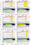 |
Fig. 1 MAVEN measurements of six inbound crossings, including Case A and Case B in Sects. 3.2 and 3.3, to show the features used to identify the PDR. The panels, from top to bottom, in each event are (a) the measurements and (b–c) the smoothed data of the magnetic field strength from MAG instrument (in black) and proton number density from SWIA (in red in panel a), (d) the three-component magnetic field in LMN coordinates, (e) the spectrum of the protons from SWIA, (f) the ion densities from STATIC instrument, and (g) the value of plasma beta (β, the ratio of thermal pressure to magnetic pressure). For each event, the red arrow labelled “BS” marks the position of the bow shock, and the horizontal colour bars stand for the PDR (in purple) and TD (in red) bounded by the two verticaldashed lines. The red lines in panels b and c represent the linear fitting lines of the smoothed |B| and
|


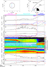 |
Fig. 2 Overview of the selected MAVEN observations from solar wind to Martian induced magnetosphere near the subsolar point on 29 September 2015. The MAVEN orbits in (a) Y –Z and (b) X–R planes in theMSO coordinates, where |
3.3 Case B on 14 February 2015
An inbound passing of MAVEN through the Martian boundaries near the terminator is illustrated in Fig. 4, in the same format as Fig. 2. MAVEN encounters the bow shock at 13:01:30 UT (marked by the left-most dashed line)and then enters the turbulent, high-density and low-velocity magnetosheath (Figs. 4c, e and j). Until 13:20:00 UT, the magnetosheath magnetic field is rather constant at a magnitude of ~17 nT with a fluctuation amplitude of more than 5 nT (Fig. 4c). According to a previous study, these fluctuations may be low-frequency waves, such as Alfvén waves (Ruhunusiri et al. 2016). The abrupt change of ions at 13:06:00 UT is caused by the mode shift of SWIA (Figs. 4e and g), which can also be affirmed by the smooth data of STATIC (Fig. 4h). When the magnetic field piles up from 13:20:00 UT to 13:29:32 UT, the amplitude of the fluctuation decreases, and the magnetic field magnitude increases steadily from 20 to 35 nT (Fig. 4c). The number density of the solar wind ions decreases from ~15 to ~3 cm−3 (Fig. 4e). The loss of the solar wind ions depends strongly on the energy, that is, the ions first get lost in the high-energy channel (Fig. 4g). The electron flux in the PDR region shows a similar feature withthe ion flux (Figs. 4g and i), namely the lost of ions and electrons starting from the high–energy channel, consistent with Øieroset et al. (2004). When the magnetic field stops increasing at 13:29:32 UT, its direction takes a sharp rotation, which is identified as a TD (Fig. 4d). The dominant composition of ions changes from solar wind ions (e.g. H+, He+) to ionospheric ions (e.g. O+, O ; Fig. 4h). After 13:33:00 UT, the magnetic field magnitude then drops a little (Fig. 4c).
Figure 5 shows the properties of the magnetic field and plasma in LMN coordinates when MAVEN passes through the PDR and TD near the terminator in the same format as Fig. 3. In the PDR, the magnetic field is piled up (Fig. 5a) with the depletion of proton ions (Fig. 5c). The temperature decreases but T⊥ ∕T∥ increases, indicating the same compression process as that of case A (Fig. 5b). Subsequently, MAVEN crosses the TD identified by the insignificant BN and reversed BL (Fig. 5b). The normal component BN is less than 5 nT with an average of 1.9 nT, but the BL component changes dramatically from 32 nT to −28 nT (Figs. 5b and k). As illustrated in the hodogram, the magnetic field vectors rotate 135° in the BM -BL plane (Fig. 5l). The  at TD is 26.4 km, while
  is 54.5 km. The average gyroradius of ions is calculated using the magnetic field magnitude and the average ion energy from MAVEN on the two sides of TD (|B1| = 33.3 nT,
  = 37 eV; |B2| = 30 nT,
  = 9 eV). The ionospheric components dominate in the overlapping region because they have larger gyroradii in this case. The hot protons cannot lead to a deep penetration.
The enhancement of the magnetic field strength starts from the outer edge of the PDR and then ends inside the induced magnetosphere. At the planet side of the TD, the magnitude of magnetic field can either continue to increase as in case A or turn to decrease as in case B.
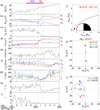 |
Fig. 3 Zoom-in plot of magnetic field and plasma parameters around the PDR and TD. (a) Magnitude and (b) three-component magnetic field in the LMN coordinate system. (c) Number density of protons from SWIA. (d) Ion components from STATIC. (e) Speed and (f) velocity of protons in the LMN coordinates. (g) Three-component proton temperature. (h) Ratio of perpendicular temperature to parallel temperature of protons from SWIA. (i) Plasma beta. (j) MAVEN position (red start) with respect to Trotignon’s MPB model (black curve; Trotignon et al. 2006) in the X–R plane, where |

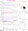 |
Fig. 5 Same format as Fig. 3 except that MAVEN passes through the duskside on 14 February 2015. The rotation angle from B1 to B2 is 135°, and |⟨BN⟩∕B0| = 0.063. |
4 Statistical results
4.1 BN /B0 distribution of discontinuity
To investigate the properties of TDs, we analyse the MAVEN measurements of 12 months from 1 January 2015 to 31 December 2015. The criteria to select discontinuities between the magnetosheath and Martian induced magnetosphere for statistical studies are described as follows:
- (1)
As the transition boundary separating the magnetosheath and IM, the candidate discontinuities should be located in the Marsward of the PDR near the ICB.
- (2)
In the statistical study, only cases with λ2∕λ3 ≥ 3 of the MVAB method (Sonnerup & Cahill 1967) are selected.
- (3)
In order to derive reliable BN components, the edges of the discontinuity are identified by sudden change in the L direction of the magnetic field.
Figure 6, from left to right, shows the global distributions of the MAVEN spacecraft orbits, identified discontinuities with λ2 ∕λ3 ≥ 3 including TDs and RDs, the ratio of the λ2∕λ3 ≥ 3 crossings ( ) to the total crossings (NB), and the ratio of the λ2∕λ3 < 3 crossings (
 ) to NB in each 0.15 × 0.15 RM bin during 2015.As shown in the left column of Fig. 6, MAVEN provides sufficient spatial coverage around Mars to study the features of the boundaries. Although the MAVEN whole orbit coverage shows a clear dawn–dusk asymmetry, such asymmetry is not significant near the magnetosheath inner boundary (Fig. 6a). In addition, to minimise the effect of the orbit coverage, the following statistics are based on the occurrence and the average results. The discontinuities between the magnetosheath and Martian induced magnetosphere used in the following statistical study are manually selected based on the three criteria above. The extremely oscillating boundary crossings are excluded, and a total of 3332 boundary crossings are identified. There is an obvious day–night asymmetry in the occurrence rate of boundaries with λ2 ∕λ3 < 3 as clearly shown in the last column of Fig. 6. The occurrence rates of boundaries with
  are larger in the nightside (XMSO < 0) than those in the dayside (XMSO > 0), suggesting that the dayside boundaries are more stable. The reason is probably that the stronger mass-loading effect at dayside can more solidly anchor the magnetic field lines, while the magnetic field lines across the boundaries at nightside are more turbulent.
These discontinuities, analogous to the Earth’s magnetopause (Eastman & Christon 2013), can be divided into two types: TD and RD. Figure 7 displays the histogram of |BN /B0|, where BN is the average normal component of magnetic field in the TD and B0 stands for the average magnetic field strength on both sides of the TD. The discontinuities in Fig. 7 are from λ2 ∕λ3 ≥ 3 discontinuities in the second column of Fig. 6. As |BN /B0| increases, the number of samples decreases gradually. The number of TDs (|BN∕B0|≤ 0.1) is about 30% and the number of potential TDs (0.1 < |BN∕B0|≤ 0.2) is about 22.4%. These jointly account for 52.4% of the λ2∕λ3 ≥ 3 events.
Figure 8 shows the global distributions of the occurence of TDs (left) and potential TDs (right), the ratio of TD/potential TD numbers from Fig. 7 to the total boundary crossing numbers. The day-side TDs are mainly distributed near the magnetopause, whereas the night-side TDs are distributed over a broader area (Fig. 8a). There is no obvious north–south asymmetry in the global distributions of TDs and potential TDs (Fig. 8d), indicating that crustal field does not play a crucial role in the formation of TDs. We note that the number of TDs is generally several times larger than that of potential TDs in almost all areas, but they have very similar global distributions.
Although the locations of TDs and potential TDs are scattered and display no obvious north–south asymmetry in the distribution coverage (Fig. 8 and black dots in Fig. 9) due to the flapping of the boundaries, their average locations are at higher altitudes in the southern hemisphere than in the northern hemisphere at dayside (colour-coded dots in Fig. 9). This is consistent with previous studies showing that the inner boundary of the magnetosheath is raised by the crustal fields (Crider et al. 2002; Matsunaga et al. 2017).
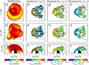 |
Fig. 6 Global distributions of MAVEN orbits used in this study. (a–c) Total orbits (Nsc). (d–f) Crossings of discontinuities between the magnetosheath and Martian induced magnetosheath with λ2 ∕λ3 ≥ 3 ( |


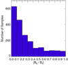 |
Fig. 7 Histogram of BN∕B0, where BN stands for the average value of the normal component of magnetic field in the discontinuity between the magnetosheath and Martian induced magnetosheath and B0 stands for the average value of the magnetic field magnitude on both sides of the discontinuity. |
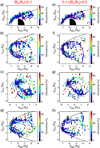 |
Fig. 8 From top to bottom: global distributions in the X–R, X–Y, Y –Z, and X–Z planes in MSO coordinates for TDs (|BN∕B0|≤ 0.1; left) and potential TDs (0.1 < |BN∕B0|≤ 0.2; right), respectively. |
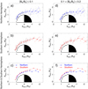 |
Fig. 9 Observed locations of the (a–c) TDs (|BN∕B0|≤ 0.1; left) and (d–f) potential TDs (0.1 < |BN∕B0|≤ 0.2; right) in MSO coordinates, where |

4.2 Thickness and rotation angle of the TD
The histogram of the corresponding thickness given in Fig. 10 is based on the distribution in Fig. 8. It should be pointed out that the thicknesses of TDs are difficult to estimate precisely using single-spacecraft observations. Here, we assume that the discontinuity is quasi-steady with respect to Mars because most events are in the quiet solar wind and the extremely oscillating boundary crossings are excluded, as pointed out above. Under this assumption, the thickness of each TD is calculated as the duration of the TD multiplied by the speed of the spacecraft in the normal direction of the TD. In ~80% of the cases, the thicknesses of TDs and potential TDs lie between 50 and 400 km, with medians of 208.4 and 194.5 km, respectively (Figs. 10a and c). Figures 10b and d show the thicknesses scaled to the proton gyroradii ( ) derived from the proton temperature at the upstream edge of these discontinuities. The median scaled thicknesses of TDs and potential TDs are both 2.0
  , ranging mostly from 0.2 to 4
  (~70%). These are much thinner than the TDs at the Earth’s magnetopause whose average thickness is supposed to be ~10
  and ~700 km (Lee & Kan 1979; Berchem & Russell 1982; Paschmann et al. 2018).
The rotation angles of TDs and potential TDs are shown in Fig. 11 based on the MAVEN orbits in Fig. 8. The rotation angle (θ) represents the angle between the magnetic field vectors on both sides of the TDs and potential TDs and is calculated using 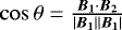 . The general distributions of rotation angles both decrease with increasing angle. The distribution of TD rotation angles has two peaks at ~0° and ~150° (Fig. 11a), whereas the distribution of potential TD rotation angles peaks at ~ 30° (Fig. 11b).
Figures 12 and 13 show the global distributions of the average thicknesses of TDs and potential TDs in kilometers and scaled to  , respectively. The formats are the same as in Fig. 8. The bins with less than three samples are not shown. The statistical results show that the day-side TDs are thinner than the night-side TDs, which is probably due to the magnetic field compression at dayside and the magnetic field stretch at nightside (Fig. 12a). The thickness scaled to
  is larger at dayside than that at nightside (Fig. 13a). The TD thickness scaled by both kilometers and
  is thicker at duskside (southern) than at dawnside (northern) (Figs. 12b and 13b; Figs. 12d and 13d). The dawn–dusk asymmetry is probably caused by the Parker spiral geometry of the solar wind magnetic field. The north–south asymmetry is more obvious when the thicknesses are scaled by
  (Figs. 12d and 13d), owing to stronger crustal magnetic fields and smaller
  in the southern hemisphere. Similar thickness distributions are also found for the potential TDs.
Figure 14 shows the global distributions of the rotation angles (θ) across TDs and potential TDs in the same formats as Fig. 8. Obviously, the dayside TDs have smaller rotation angles than the nightside TDs, and the TDs closer to Mars have larger rotation angles (Fig. 14a). Similar to the distributions of TD thickness, obvious dawn–dusk asymmetry (Fig. 14b) and invisible south–north asymmetry (Fig. 14d) are found in the distributions of TD rotation angle. The rotation angles of dawn-side TDs are slightly larger than those of dusk-side TDs (Fig. 14b), and the southern TDs are not significantly influenced by the crustal magnetic field (Fig. 14d). The TD rotation angles can be larger than 90° in the nightside and duskside, meaning that the magnetic fields of most TDs in these regions reverse on the two sides of these TDs. The potential TDs have similar rotation angle distributions. Overall, rotation angle is distributed in a similar way to the thickness, revealing that thicker TDs have larger rotation angles.
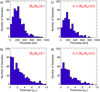 |
Fig. 10 Histograms of discontinuity thicknesses of (a) TDs in kilometers, (b) potential TDs, (c) TDs scaled to the proton gyroradius, and (d) potential TDs scaled to the proton gyroradius. |
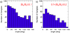 |
Fig. 11 Histograms of the rotation angle besides the discontinuity for (a) TDs (|BN∕B0|≤ 0.1) and (b) potential TDs (0.1 < |BN∕B0|≤ 0.2). |

4.3 Statistical results for the PDR
The statistical characteristics of the PDR upstream of the TD (|BN∕B0|≤ 0.1) are shown in Figs. 15 and 16. The leading boundary of the PDR is automatically identified by the method described in Sect. 3.3. The PDLs upstream of Earth’s magnetopause are detectedmore frequently in the northward IMF than in the southward IMF (Wang et al. 2004). Magnetic reconnection which can produce a RD is more easily triggered in the southward IMF. During this process, the piled-up magnetic field is dragged away in the PDL. Thus, the structures of PDLs are influenced upstream of the RDs. A similar process could also happen for PDRs at Mars. Therefore, only the PDRs upstream of TDs are shown in this study.
Figure 15 shows the distribution of the PDR thickness upstream of the TD in MSO coordinates. The blue and red bars show the average PDR thicknesses and directions in the northern and southern hemisphere, respectively (Figs. 15a and c). The PDRs are thicker at nightside than at dayside in both northern and southern hemispheres, consistent with the day–night asymmetry of the whole magnetosheath thickness. In the dayside, the PDRs are thicker in the northern hemisphere than in the southern hemisphere, indicating that the crustal magnetic fields compress the southern magnetosheath by lifting the inner boundary of the magnetosheath (north–south asymmetry of TDs in Fig. 9).
Figure 16 shows the statistical features of the PDR depending on SZA. With the increase of SZA, both the proton number density and temperature from SWIA decrease, resulting from the weak compression in the tailward magnetosheath, consistent with the increase of the PDR thickness. In the tailward, the plasma beta (β, the ratio of thermal pressure to magnetic pressure) increases while the thermal pressure decreases (derived from the decrease of both proton number density and temperature), indicating that the magnetic field pressure decreases faster than the thermal pressure.
There are also north–south asymmetries in the distributions of these physical parameters within the PDR. In the southern hemisphere, the proton number densities are larger but the proton temperatures are lower. Although the crustal magnetic field leads to stronger compression and higher proton number density in the southern magnetosheath, more higher-energy protons depleted from the PDR along the piled-up magnetic field leads to lower proton temperatures.
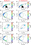 |
Fig. 14 Same format as Fig. 8 except for the average rotation angle of the magnetic field across TDs and potential TDs. |
5 Discussion
5.1 Comparison with Earth
Although Mars has no global intrinsic magnetic field, the structures upstream of Mars are similar to those around Earth. They both have the bow shock, magnetosheath (containing PDL/PDR), discontinuity (TD/RD), and magnetosphere or induced magnetosphere.
The PDL associated with the compression of the magnetic field on the sunward side of Earth’s magnetopause has been studied for a long time using both in situ observations (e.g. Anderson et al. 1994; Crooker et al. 1979; Sibeck et al. 1990)and simulations (e.g. Farrugia et al. 1997; Wang et al. 2004; Wu 1992; Zwan & Wolf 1976). Øieroset et al. (2004) suggested that the MPB with piled-up magnetic field upstream of Mars resembles the Earth’s PDL. However, without the detection of ion composition, this cannot be confirmed. Using the measurements from STATIC/MAVEN, we find that the ion composition in the region where the magnetic field is compressed and the plasma is depleted is mainly protons from solar wind. This indicates that this region is part of the magnetosheath. In addition, the behaviour of the plasma in this region is similar to that in Earth’s PDL, with an enhancement of T⊥ ∕T∥.
The Earth’s magnetopause consists of a discontinuity (TD or RD) resulting from the change in orientation and magnitude between the IMF and Earth’s intrinsic magnetic field, which has been observed by spacecraft (e.g. Eastman & Christon 2013; Paschmann et al. 2018; Haaland et al. 2019) and studied using models and simulations (e.g. Lee & Kan 1979; Swift & Lee 1982). The plasma composition on the two sides of the Earth’s magnetopause changes from the magnetosheath protons to the hotter H+ and O+ ions (Bouhram et al. 2005). A similar structure of discontinuity is also found between the Martian magnetosheath and the induced magnetosphere as demonstrated in the present paper. The magnetic field changes its orientation and magnitude across the discontinuity. From the sun-side to Mars-side of the discontinuities, the dominated ion composition changes from protons of the shocked solar wind to the heavy ions originating from the Martian ionosphere.
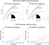 |
Fig. 15 Average thicknesses of the PDR upstream of the TD (|BN∕B0|≤ 0.1) (a–b) in MSO coordinates, where |
5.2 Formation of the discontinuity
Like the Earth’s magnetopause, the discontinuity separates the Martian magnetosheath and the induced magnetosphere. When the shocked solar wind travels anti-sunward toward the Martian ionosphere/atmosphere, it is slowed down by the mass-loading process associated with the heavy ions of planetary origin. The solar wind magnetic fields drape around Mars and form the induced magnetosphere. The magnetic field pattern in the Martian induced magnetosphere is mainly determined by the orientation of the IMF. When this latter changes, the magnetic fields on the two sides of the boundary are expected to have different directions, leading to formation of the TD. The magnetic field rotates within the TD transition region. At the Earth’s magnetopause, the discontinuity is identified either as a TD or as a RD after reconnection (Lee & Kan 1979; Eastman et al. 1996; Sonnerup & Cahill 1967). At Mars, the discontinuity between the magnetosheath and Martian induced magnetosphere also has these two types.
At dayside, the magnetic field lines that are heavily mass loaded stay relatively fixed in place though they convect downstream and become a part of the induced magnetosphere. Meanwhile, these magnetic fields can prevent most solar wind protons from entering into the induced magnetosphere, leading to the formation of the ICB. Therefore, the magnetic discontinuity between the magnetosheath and the induced magnetosphere should be located in the same place as the ICB. The induced magnetosphere of Mars, into which solar wind particles barely enter, can be treated as a part of Mars, analogous to the Earth’s intrinsic magnetosphere. This is probably why Mars and Earth have the same structures when interacting with solar wind.
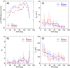 |
Fig. 16 Solarzenith angle (SZA) dependence of (a) crossing numbers, (b) median plasma beta (β, the ratio of thermal pressure to magnetic pressure), (c) median proton number density ( |


6 Conclusion
The major results of our analysis of the structures upstream of Mars based on the MAVEN measurements can be summarised as follows:
- (1)
As shown in Fig. 17, when a spacecraft moves inward from the solar wind, it enters the magnetosheath throughthe bow shock, then encounters the magnetopause, and finally reaches the IM. The inner part of magnetosheath is called the PDR, similar to the PDL upstream of the Earth’s magnetopause, in which the magnetic field is compressed and the plasma density is depleted.
- (2)
In the outer part of the magnetosheath, the magnetic field and plasma density fluctuate around constant values. Several types of waves can be observed in this region, such as fast mode waves or mirror mode waves.
- (3)
The PDR is at the inner part of the magnetosheath. As the magnetic field piles up, its fluctuation weakens, and the plasma of the magnetosheath is squeezed out along the magnetic field. Although the plasma beta and proton number density decrease, the magnetosheath plasma is still the dominant composition. This region has been identified as MPB or IMB previously due to the sudden enhancement of magnetic field magnitude.
- (4)
Due to the escape of hotter plasma along the magnetic field in the PDR, the proton temperature decreases while T⊥∕T∥ increases. The mirror mode waves can still occasionally be found in the PDR.
- (5)
Similar to the Earth’s magnetopause, the boundary of the Mars–solar wind interaction between the magnetosheath and the induced magnetosphere is a discontinuity, either tangential discontinuity (TD) or rotational discontinuity (RD) where the magnetic field changes its orientation. This discontinuity separates the magnetosheath H+ from the heavy ions in the induced magnetosphere. The discontinuities in the six cases presented in this paper are identified as TDs, owing to the extremely small normal component (BN). Inside the TDs, the ions from both sides are mixed but are dominated by the ionospheric ions.
- (6)
Statistical results for the discontinuities between the magnetosheath and Martian induced magnetosphere show that the TDs (|BN∕B0|≤ 0.1) and potential TDs (0.1 < |BN∕B0|≤ 0.2) are about 30 and 22.4% of the selected discontinuities with λ2∕λ3 ≥ 3. The global distributions of TDs and potential TDs indicate that the crustal field in the southern hemisphere does not play a crucial role in the formation of TDs, but raises the location of the TDs. Tangential discontinuities in the northern hemisphere can also be generated by the differences between the mass-loading IMF and the recently arrived IMF. The thickness of TDs near Mars is ~200 km, mostly inside the range of 1–10
 (100–1000 km), thinner than the Earth’s magnetopause. The rotation angle distribution of TDs has two peaks at
~0°
and ~150°, whereas the rotation angle distribution of potential TDs peaks at ~30°. The global distributions of thickness and rotation angle both show day–night and dawn–dusk asymmetries. Thicknesses are larger in the south hemisphere where the crustal field is located than in the north hemisphere, whereas rotation angle does not show an obvious north–south asymmetry.
(100–1000 km), thinner than the Earth’s magnetopause. The rotation angle distribution of TDs has two peaks at
~0°
and ~150°, whereas the rotation angle distribution of potential TDs peaks at ~30°. The global distributions of thickness and rotation angle both show day–night and dawn–dusk asymmetries. Thicknesses are larger in the south hemisphere where the crustal field is located than in the north hemisphere, whereas rotation angle does not show an obvious north–south asymmetry. - (7)
Statistical results for the PDRs in front of TDs show that thicknesses of PDRs increase while the proton number density and temperature decrease in the tailward. In the dayside, the distributions of PDR parameters show north–south asymmetries, that is, the PDRs are thinner, the proton number densities are larger, but the proton temperatures are lower in the southern hemisphere.
The discontinuities are transition regions during the interaction between the solar wind and Mars in most cases. The statistical results show that 52.4% of the discontinuities with λ2 ∕λ3 ≥ 3 are most likely TDs (|BN∕B0|≤ 0.2). In some cases, the solar wind protons can pass the discontinuities and penetrate into the IM, forming a boundary layer (BL; Eastman & Hones 1979). The properties of the rest cases of the discontinuities, such as RDs (|BN∕B0|≥ 0.2) and BLs, will be investigated in a future companion work.
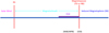 |
Fig. 17 Sketch shows the structures of boundaries upstream of Mars in the top row: solar wind, BS, magnetosheath, magnetopause, and induced magnetosphere. The magnetopause is an MHD discontinuity, either TDor RD. The inner part of magnetosheath is called the PDR, similar to the PDL at Earth, in which the magnetosheath magnetic fields are compressed and piled up, and the plasma is depleted. This PDR with enhanced magnetic field was previously identified as the IMB and the MPB. The magnetopause, that is, the TD or RD transition region, has also been referred to as the ICB, which separates H+ ions in the magnetosheath and heavy ions in the induced magnetosphere. |
Acknowledgements
This work is supported by the Science and Technology Development Fund of Macao SAR (0035/2018/AFJ), the pre-research project on Civil Aerospace Technologies No. D020308 funded by China National Space Administration, and the Ministry of Science and Technology in Taiwan (MOST 108-2111-M-002-005). We acknowledge the MAVEN contract for support. All MAVEN data are available on the Planetary Data System (https://pds.nasa.gov).
References
- Acuña, M. H., Connerney, J. E. P., Wasilewski, P., et al. 1998, Science, 279, 1676 [NASA ADS] [CrossRef] [Google Scholar]
- Anderson, B. J., Fuselier, S. A., Gary, S. P., & Denton, R. E. 1994, J. Geophys. Res., 99, 5877 [NASA ADS] [CrossRef] [Google Scholar]
- Berchem, J., & Russell, C. T. 2001, J. Geophys. Res., 87, 2108 [Google Scholar]
- Bertucci, C., Mazelle, C., Crider, D. H., et al. 2004, Adv. Space Res., 33, 1938 [NASA ADS] [CrossRef] [Google Scholar]
- Bertucci, C., Mazelle, C., & Acuña, M. H. 2005, J. Atm. Sol. -Terr. Phys., 67, 1797 [NASA ADS] [CrossRef] [Google Scholar]
- Bertucci, C., Duru, F., Edberg, N., et al. 2011, Space Sci. Rev., 162, 113 [Google Scholar]
- Brain, D., Barabash, S., Boesswetter, A., et al. 2010, Icarus, 206, 139 [NASA ADS] [CrossRef] [Google Scholar]
- Breus, T. K., Dubinin, E. M., Krymskii, A. M., et al. 1991, J. Geophys. Res., 96, 11165 [Google Scholar]
- Bouhram, M., Klecker, B., Paschmann, G., et al. 2005, Ann. Geophys., 23, 1281 [NASA ADS] [CrossRef] [Google Scholar]
- Connerney, J. E. P., Acuña, M. H., Ness, N. F., et al. 2004, Space Sci. Rev., 111, 1 [NASA ADS] [CrossRef] [Google Scholar]
- Connerney, J. E. P., Espley, J. R., DiBraccio, G. A., et al. 2015a, Geophys. Res. Lett., 42 [Google Scholar]
- Connerney, J. E. P., Espley, J., Lawton, P., et al. 2015b, Space Sci. Rev., 195, 257 [NASA ADS] [CrossRef] [Google Scholar]
- Crider, D. H., Acuña, M. H., Connerney, J. E. P., et al. 2002, Geophys. Res. Lett., 29, 11 [CrossRef] [Google Scholar]
- Crider, D., Brain, D. A., Acuña, M. H., et al. 2004, Space Sci. Rev., 111, 203 [NASA ADS] [CrossRef] [Google Scholar]
- Crooker, N. U., Eastman, T. E., & Stiles, G. S. 1979, J. Geophys. Res., 84, 869 [NASA ADS] [CrossRef] [Google Scholar]
- Dubinin, E., Lundin, R., Koskinen, H., & Norberg, O. 1993, J. Geophys. Res., 98, 5617 [NASA ADS] [CrossRef] [Google Scholar]
- Dubinin, E., Obod, D., Pedersen, A., & Grard, R. 1994, Geophys. Res. Lett., 21, 2769 [NASA ADS] [CrossRef] [Google Scholar]
- Dubinin, E., Sauer, K., Lundin, R., et al. 1996, Geophys. Res. Lett., 23, 785 [NASA ADS] [CrossRef] [Google Scholar]
- Dubinin, E., Sauer, K., Baumgärtel, K., & Lundin, R. 1997, Adv. Space Res., 20, 149 [NASA ADS] [CrossRef] [Google Scholar]
- Dubinin, E., Sauer, K., Delva, M., & Tanaka, T. 1998a, Earth, Planets Space, 50, 873 [NASA ADS] [CrossRef] [Google Scholar]
- Dubinin, E., Sauer, K., Baumgärtel, K., & Srivastava, K. 1998b, Earth, Planets Space, 50, 279 [NASA ADS] [CrossRef] [Google Scholar]
- Dubinin, E., Lundin, R., Fränz, M., et al. 2006, Icarus, 182, 337 [NASA ADS] [CrossRef] [Google Scholar]
- Dubinin, E., Modolo, R., Fraenz, M., et al. 2008, Geophys. Res. Lett., 35, L11103 [NASA ADS] [CrossRef] [Google Scholar]
- Dubinin, E., Fraenz, M., Pätzold, et al. 2018, Geophys. Res. Lett., 45, 2574 [CrossRef] [Google Scholar]
- Eastman, T., & Christon, S. 2013, Physics of the Magnetopause, eds. P. Song, B. Sonnerup, & M. Thomsen (Washington, D.C.: American Geophysical Union) [Google Scholar]
- Eastman, T. E., & Hones, E. W. 1979, J. Geophys. Res., 84, 2019 [NASA ADS] [CrossRef] [Google Scholar]
- Eastman, T. E., Fuselier, S. A., & Gosling, J. T. 1996, J. Geophys. Res., 101, 49 [CrossRef] [Google Scholar]
- Espley, J. R., Cloutier, P. A., Brain, D. A., et al. 2004, J. Geophys. Res., 109, A07213 [NASA ADS] [Google Scholar]
- Farrugia, C. J., Erkaev, N. V., Biernat, H. K., Lawrence, G. R., & Elphic, R. C. 1997, J. Geophys. Res., 102, 315 [Google Scholar]
- Haaland, S., Runov, A., Artemyev, A., & Angelopoulos, V. 2019, J. Geophys. Res., 124, 3421 [NASA ADS] [CrossRef] [Google Scholar]
- Halekas, J., Taylor, E., Dalton, G., et al. 2015, Space Sci. Rev., 195, 125 [CrossRef] [Google Scholar]
- Halekas, J. S, Ruhunusiri, S., Harada, Y., et al. 2016, J. Geophys. Res. Space Phys., 122, 547 [NASA ADS] [CrossRef] [Google Scholar]
- Halekas, J. S., Brain, D. A., Luhmann, J. G., et al. 2017, J. Geophys. Res. Space Phys., 122, 341 [Google Scholar]
- Hall, B. E. S., Lester, M., Sänchez-Cano, B., et al. 2016, J. Geophys. Res. Space Phys., 121, 474 [Google Scholar]
- Hampel, F. R. 1974, J. Am. Stat. Assoc., 69, 383 [CrossRef] [Google Scholar]
- Hantsch, M. H., & Bauer, S. J. 1990, Planet. Space Sci., 38, 539 [NASA ADS] [CrossRef] [Google Scholar]
- Hasegawa, A. 1969, Phys. Fluids, 12, 2642 [CrossRef] [Google Scholar]
- Holmberg, M. K. G., Andre, N., Garnier, P., et al. 2019, J. Geophys. Res. Space Phys., 124, 8564 [Google Scholar]
- Jakosky, B. M., Grebowsky, J. M., Luhmann, J. G., & Brain, D. A. 2015, Geophys. Res. Lett., 42 [Google Scholar]
- Kallio, E., Koskinen, H., Barabash, S., et al. 1994, J. Geophys. Res., 99, 23547 [NASA ADS] [CrossRef] [Google Scholar]
- Landau, L. D., & Lifshil, E. M., 1959, Fluid Mechanics (London: Pergamon) [Google Scholar]
- Lee, L. C., & Kan, J. 1979, J. Geophys. Res., 84, 6417 [NASA ADS] [CrossRef] [Google Scholar]
- Lin, Y., & Lee, L. C., 1993, Space Sci. Rev., 65, 59 [Google Scholar]
- Lundin, R., Dubinin, E. M., Koskinen, H., et al. 1991, Geophys. Res. Lett., 18, 1059 [NASA ADS] [CrossRef] [Google Scholar]
- Matsunaga, K., Seki, K., Hara, T., & Brain, D. A. 2015, J. Geophys. Res. Space Phys., 120, 6874 [Google Scholar]
- Matsunaga, K., Seki, K., Brain, D. A., et al. 2017, J. Geophys. Res. Space Phys., 122 [Google Scholar]
- Mazelle, C., Réme, H., Sauvaud, J. A., et al. 1989, Geophys. Res. Lett., 16, 1035 [NASA ADS] [CrossRef] [Google Scholar]
- Mazelle, C., Winterhalter, D., Sauer, K., et al. 2004, Space Sci. Rev., 111, 115 [NASA ADS] [CrossRef] [Google Scholar]
- McFadden, J. P., Kortmann, O., Curtis, D., et al. 2015, Space Sci. Rev., 195, 199 [CrossRef] [Google Scholar]
- Mitchell, D. L., Mazelle, C., Sauvaud, J.-A., et al. 2016, Space Sci. Rev., 200, 495 [NASA ADS] [CrossRef] [Google Scholar]
- Nagy, A. F., Winterhalter, D., Sauer, K., et al. 2004, Space Sci. Rev., 111, 33 [NASA ADS] [CrossRef] [Google Scholar]
- Øieroset, M., Mitchell, D., Phan, T., et al. 2004, Space Sci. Rev., 111, 185 [CrossRef] [Google Scholar]
- Paschmann, G., Haaland, S. E., Phan, T. D., et al. 2018, J. Geophys. Res. Space Phys., 123, 2018 [NASA ADS] [Google Scholar]
- Riedler, W., Schwingenschuh, K., Moehlmann, D., et al. 1989, Nature, 341, 604 [NASA ADS] [CrossRef] [Google Scholar]
- Ruhunusiri, S., Halekas, J. S., McFadden, J. P., et al. 2016, Geophys. Res. Lett., 43, 4763 [NASA ADS] [CrossRef] [Google Scholar]
- Russell, C.T. 1979, ASP Sol. Syst. Plasma Phys., 2, 208 [NASA ADS] [Google Scholar]
- Russell, C.T., & Elphic, R. C. 1978, Space Sci. Rev., 22, 681 [NASA ADS] [CrossRef] [Google Scholar]
- Sauer, K., Bogdanov, A., & Baumgartel, K. 1994, Geophys. Res. Lett., 21, 2255 [NASA ADS] [CrossRef] [Google Scholar]
- Sauer, K., Dubinin, E., & Baumgärtel, K. 1998, Earth, Planets Space, 50, 793 [NASA ADS] [CrossRef] [Google Scholar]
- Schwartz, S. J., Andersson, L., Xu, S., et al. 2019, Geophys. Res. Lett., 46, 7157 [Google Scholar]
- Sibeck, D. G., Lepping, R. P., & Lazarus, A. J. 1990, J. Geophys. Res., 95, 2433 [NASA ADS] [CrossRef] [Google Scholar]
- Skalsky, A., Dubinin, E. M., Petrukovich, A., et al. 1998, Earth Planets Space, 50, 289 [NASA ADS] [CrossRef] [Google Scholar]
- Slavin, J. A., & Holzer, R. E. 1982, J. Geophys. Res., 87, 10285 [NASA ADS] [CrossRef] [Google Scholar]
- Sonnerup, B. U., & Ledley, B. G. 1974, J. Geophys. Res., 79, 4309 [NASA ADS] [CrossRef] [Google Scholar]
- Sonnerup, B. U., & Cahill, L. J. 1967, J. Geophys. Res., 72, 171 [NASA ADS] [CrossRef] [Google Scholar]
- Swift, D. W., & Lee, L. C. 1982, Geophys. Res. Lett., 9, 527 [NASA ADS] [CrossRef] [Google Scholar]
- Szego, K., Glassmeier, K.-H., Bingham, R., et al. 2000, Space Sci. Rev., 94, 429 [NASA ADS] [CrossRef] [Google Scholar]
- Trotignon, J. G., Dubinin, E., Grard, R., et al. 1996, J. Geophys. Res., 101, 24965 [CrossRef] [Google Scholar]
- Trotignon, J. G., Mazelle, C., Bertucci, et al. 2006, Planet. Space Sci., 54, 357 [Google Scholar]
- Tsurutani, B. T., Smith, E. J., Anderson, R. R., et al. 1982, J. Geophys. Res., 87, 6060 [NASA ADS] [CrossRef] [Google Scholar]
- Vignes, D., Mazelle, C., Rme, H., et al. 2000, Geophys. Res. Lett., 27, 49 [NASA ADS] [CrossRef] [Google Scholar]
- Wang, D., Vagnucci, A., & Li, C. C. 1981, Comput. Graph. Image Process., 15, 167 [CrossRef] [Google Scholar]
- Wang, Y. L., Raeder, J., & Russell, C. T., 2004, Ann. Geophys., 22, 1001 [NASA ADS] [CrossRef] [Google Scholar]
- Wu, C. C. 1992, Geophys. Res. Lett., 19, 87 [NASA ADS] [CrossRef] [Google Scholar]
- Xu, S., Liemohn, M. W., Dong, C., et al. 2016, J. Geophys. Res. Space Phys., 121, 6417 [NASA ADS] [CrossRef] [Google Scholar]
- Zwan, B. J., & Wolf, R. A. 1976, J. Geophys. Res., 81, 1636 [NASA ADS] [CrossRef] [Google Scholar]
All Figures
|
Fig. 1 MAVEN measurements of six inbound crossings, including Case A and Case B in Sects. 3.2 and 3.3, to show the features used to identify the PDR. The panels, from top to bottom, in each event are (a) the measurements and (b–c) the smoothed data of the magnetic field strength from MAG instrument (in black) and proton number density from SWIA (in red in panel a), (d) the three-component magnetic field in LMN coordinates, (e) the spectrum of the protons from SWIA, (f) the ion densities from STATIC instrument, and (g) the value of plasma beta (β, the ratio of thermal pressure to magnetic pressure). For each event, the red arrow labelled “BS” marks the position of the bow shock, and the horizontal colour bars stand for the PDR (in purple) and TD (in red) bounded by the two verticaldashed lines. The red lines in panels b and c represent the linear fitting lines of the smoothed |B| and
|
| In the text | |
|
Fig. 2 Overview of the selected MAVEN observations from solar wind to Martian induced magnetosphere near the subsolar point on 29 September 2015. The MAVEN orbits in (a) Y –Z and (b) X–R planes in theMSO coordinates, where |
| In the text | |
|
Fig. 3 Zoom-in plot of magnetic field and plasma parameters around the PDR and TD. (a) Magnitude and (b) three-component magnetic field in the LMN coordinate system. (c) Number density of protons from SWIA. (d) Ion components from STATIC. (e) Speed and (f) velocity of protons in the LMN coordinates. (g) Three-component proton temperature. (h) Ratio of perpendicular temperature to parallel temperature of protons from SWIA. (i) Plasma beta. (j) MAVEN position (red start) with respect to Trotignon’s MPB model (black curve; Trotignon et al. 2006) in the X–R plane, where |
| In the text | |
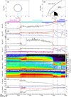 |
Fig. 4 Same format as Fig. 2 except that MAVEN passes through the duskside on 14 February 2015. |
| In the text | |
|
Fig. 5 Same format as Fig. 3 except that MAVEN passes through the duskside on 14 February 2015. The rotation angle from B1 to B2 is 135°, and |⟨BN⟩∕B0| = 0.063. |
| In the text | |
|
Fig. 6 Global distributions of MAVEN orbits used in this study. (a–c) Total orbits (Nsc). (d–f) Crossings of discontinuities between the magnetosheath and Martian induced magnetosheath with λ2 ∕λ3 ≥ 3 ( |
| In the text | |
|
Fig. 7 Histogram of BN∕B0, where BN stands for the average value of the normal component of magnetic field in the discontinuity between the magnetosheath and Martian induced magnetosheath and B0 stands for the average value of the magnetic field magnitude on both sides of the discontinuity. |
| In the text | |
|
Fig. 8 From top to bottom: global distributions in the X–R, X–Y, Y –Z, and X–Z planes in MSO coordinates for TDs (|BN∕B0|≤ 0.1; left) and potential TDs (0.1 < |BN∕B0|≤ 0.2; right), respectively. |
| In the text | |
|
Fig. 9 Observed locations of the (a–c) TDs (|BN∕B0|≤ 0.1; left) and (d–f) potential TDs (0.1 < |BN∕B0|≤ 0.2; right) in MSO coordinates, where |
| In the text | |
|
Fig. 10 Histograms of discontinuity thicknesses of (a) TDs in kilometers, (b) potential TDs, (c) TDs scaled to the proton gyroradius, and (d) potential TDs scaled to the proton gyroradius. |
| In the text | |
|
Fig. 11 Histograms of the rotation angle besides the discontinuity for (a) TDs (|BN∕B0|≤ 0.1) and (b) potential TDs (0.1 < |BN∕B0|≤ 0.2). |
| In the text | |
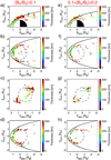 |
Fig. 12 Same format as Fig. 8 but the average thickness is given in kilometers. |
| In the text | |
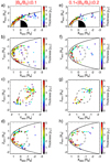 |
Fig. 13 Same format as Fig. 8 except that the average thickness is scaled by
|
| In the text | |
|
Fig. 14 Same format as Fig. 8 except for the average rotation angle of the magnetic field across TDs and potential TDs. |
| In the text | |
|
Fig. 15 Average thicknesses of the PDR upstream of the TD (|BN∕B0|≤ 0.1) (a–b) in MSO coordinates, where |
| In the text | |
|
Fig. 16 Solarzenith angle (SZA) dependence of (a) crossing numbers, (b) median plasma beta (β, the ratio of thermal pressure to magnetic pressure), (c) median proton number density ( |
| In the text | |
|
Fig. 17 Sketch shows the structures of boundaries upstream of Mars in the top row: solar wind, BS, magnetosheath, magnetopause, and induced magnetosphere. The magnetopause is an MHD discontinuity, either TDor RD. The inner part of magnetosheath is called the PDR, similar to the PDL at Earth, in which the magnetosheath magnetic fields are compressed and piled up, and the plasma is depleted. This PDR with enhanced magnetic field was previously identified as the IMB and the MPB. The magnetopause, that is, the TD or RD transition region, has also been referred to as the ICB, which separates H+ ions in the magnetosheath and heavy ions in the induced magnetosphere. |
| In the text | |
Current usage metrics show cumulative count of Article Views (full-text article views including HTML views, PDF and ePub downloads, according to the available data) and Abstracts Views on Vision4Press platform.
Data correspond to usage on the plateform after 2015. The current usage metrics is available 48-96 hours after online publication and is updated daily on week days.
Initial download of the metrics may take a while.