| Issue |
A&A
Volume 641, September 2020
|
|
|---|---|---|
| Article Number | L5 | |
| Number of page(s) | 10 | |
| Section | Letters to the Editor | |
| DOI | https://doi.org/10.1051/0004-6361/202038769 | |
| Published online | 04 September 2020 | |
Letter to the Editor
Signatures of ubiquitous magnetic reconnection in the lower solar atmosphere⋆
1
Institute of Theoretical Astrophysics, University of Oslo, PO Box 1029, Blindern 0315, Oslo, Norway
e-mail: This email address is being protected from spambots. You need JavaScript enabled to view it.
2
Rosseland Centre for Solar Physics, University of Oslo, PO Box 1029, Blindern 0315, Oslo, Norway
3
Institute for Solar Physics, Dept. of Astronomy, Stockholm University, AlbaNova University Centre, 10691 Stockholm, Sweden
Received:
26
June
2020
Accepted:
28
July
2020
Abstract
Ellerman Bomb-like brightenings of the hydrogen Balmer line wings in the quiet Sun, also known as quiet Sun Ellerman bombs (QSEBs), are a signature of the fundamental process of magnetic reconnection at the smallest observable scale in the lower solar atmosphere. We analyze high spatial resolution observations (0.″1) obtained with the Swedish 1-m Solar Telescope to explore signatures of QSEBs in the Hβ line. We find that QSEBs are ubiquitous and uniformly distributed throughout the quiet Sun, predominantly occurring in intergranular lanes. We find up to 120 QSEBs in the field of view for a single moment in time; this is more than an order of magnitude higher than the number of QSEBs found in earlier Hα observations. This suggests that about half a million QSEBs could be present in the lower solar atmosphere at any given time. The QSEB brightenings found in the Hβ line wings also persist in the line core with a temporal delay and spatial offset toward the nearest solar limb. Our results suggest that QSEBs emanate through magnetic reconnection along vertically extended current sheets in the lower solar atmosphere. The apparent omnipresence of small-scale magnetic reconnection may play an important role in the energy balance of the solar chromosphere.
Key words: Sun: activity / Sun: atmosphere / Sun: magnetic fields
Movies associated to Figs. 1−3, B1, and B2 are available at https://www.aanda.org
© ESO 2020
1. Introduction
Magnetic reconnection is at the root of a wide range of magnetic activity phenomena in the solar atmosphere and is the fundamental driver of, for example, solar flares and coronal mass ejections. In the deep solar atmosphere, magnetic reconnection is manifested as Ellerman bombs (EBs): small but intense brightenings of the extended wings of the hydrogen Balmer-α line (Hα). EBs are traditionally found in complex bipolar active regions, particularly during episodes of vigorous flux emergence; they are invisible in the Hα line core, which locates the site of reconnection below the chromospheric canopy of fibrils (Watanabe et al. 2011; Vissers et al. 2013).
The advanced numerical simulations of Hansteen et al. (2017, 2019) and Danilovic (2017) have reinforced the interpretation of EBs as markers of small-scale photospheric magnetic reconnection. EBs are further characterized as a transient phenomenon with lifetimes on the order of minutes and a morphology in slanted-view Hα-wing images that appears like flames: bright, upright, 1–2 Mm tall, and rapidly flickering on timescales of seconds (Watanabe et al. 2011). We refer to Rutten et al. (2013) for a review of EB properties and the introduction of Vissers et al. (2019) for an overview of EB visibility in different diagnostics.
Rouppe van der Voort et al. (2016) recently discovered a phenomenon of Ellerman bomb-like brightenings in the quiet Sun, far away from regions with strong magnetic activity. These quiet Sun Ellerman bombs (QSEBs) are smaller in size and exhibit weaker enhancement of their Hα wings than their active region counterparts (Rouppe van der Voort et al. 2016; Nelson et al. 2017). QSEBs are also thought to originate through magnetic reconnection in the photosphere (Rouppe van der Voort et al. 2016; Shetye et al. 2018), similar to EBs.
Here, we further advance the observational characterization of QSEBs by analysis of high-resolution observations in the Balmer-β (Hβ) line. EBs in active regions were observed in the Hβ line by Ellerman (1917) and Libbrecht et al. (2017). The shorter wavelength of the Hβ line allows higher spatial resolution and enhanced intensity contrast compared to Hα observations. The latter stems from the wavelength dependence of the Planck function, which results in higher contrast at shorter wavelengths for the enhanced temperature in the reconnection site. We find much higher numbers of QSEBs compared to the earlier Hα observations. This apparent ubiquity of QSEBs raises interest in the impact of low atmospheric reconnection events onto the total energy budget of the solar atmosphere. Furthermore, we see evidence of a dynamical progression of the reconnection process from lower to higher altitude. These findings highlight the potential of high-resolution observations in probing the smallest observable magnetic reconnection events in the solar atmosphere.
2. Observations
The observations were obtained with the CHROMIS and CRISP (Scharmer et al. 2008) instruments at the Swedish 1-m Solar Telescope (SST, Scharmer et al. 2003) on 6 June 2019. The target was a quiet Sun region at (x, y) = (611″, 7″) and the time series has a duration of 1 h starting at 8:41 UT. CHROMIS observed the Hβ spectral line at 4861 Å with the temporal cadence of 8.6 s and a pixel scale of  . The CHROMIS instrument has an auxiliary wide-band (WB) channel that is equipped with a continuum filter centered at 4845 Å (FWHM = 6.5 Å). The analyzed WB data has the same cadence as the Hβ data. CRISP ran a program sampling the Hα, Fe I 6173 Å, and Ca II 8542 Å spectral lines at a cadence of 35.9 s. For this study, we concentrated on the Hα and Fe I 6173 Å observations. Further details of the observations, data reduction, and method to infer the line-of-sight component of the magnetic field (BLOS) are described in Appendix A.
3. Data analysis
3.1. Identification of QSEBs
Signatures of EBs and QSEBs are readily observable in the Hα and Hβ lines; the wings of these lines show enhancement, whereas the line core remains unaffected. To identify this telltale spectral signature of QSEBs, we used the k-means clustering technique (Everitt 1972) to classify the Hβ observations into 100 different line profiles. Out of the 100 Hβ line profiles, we identified profiles that show the signatures of QSEBs, i.e., the enhanced wings and unaffected line core. The red contours indicate QSEB detections in Fig. 1, which shows an example Hβ blue-wing image alongside the co-temporal continuum WB image. We will outline the details of the k-means classification methodology to identify QSEBs in a follow-up paper.
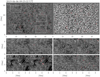 |
Fig. 1. Ubiquitous QSEB detections using the k-means clustering technique. (a) Observed FOV in the Hβ blue wing. The red contours indicate the location of QSEBs. (b) Co-temporal continuum WB image. (c–f) Zoom-in on the four different areas indicated by the white boxes in (a); each panel shows duplicate images, one with the red contours indicating the location of QSEBs and one without the contours. The arrow in panel b shows the direction of the closest solar limb. An animation of this figure is available online. |
Figure 1 shows that the QSEBs are almost uniformly distributed throughout the field of view (FOV). From the zoom-in on four different areas presented in Fig. 1, it is evident that QSEBs are predominantly located in the intergranular lanes. We found a total of ∼2800 events in 420 CHROMIS spectral scans within the FOV of 60″ × 40″. The number of detected events varies from scan to scan, clearly correlated to variations in the seeing conditions. In the highest quality scans we found up to 120 QSEBs in the FOV suggesting that there could be as many as half a million QSEBs present on the solar surface at any given time.
3.2. Selected examples of QSEBs
Quiet Sun Ellerman bombs vary significantly in their properties, such as lifetime, brightness, and size. In this study we present a few specific examples that are representative of all QSEBs, and demonstrate the variations in different properties.
The QSEB displayed in Fig. 2 is in the category of brighter, bigger, and longer-lived QSEBs. In the Hβ red-wing intensity map, the QSEB appears as a bright flame-like structure elongated in the direction of the closest solar limb. The Hβ spectra of the QSEB show the typical enhancement of the line wings while the line core remains unchanged compared to the average background spectrum. The QSEB is also visible in the intensity map obtained in the Hα red wing. However, the Hα spectra exhibit very little enhancement in the line wings. The WB image suggests that the QSEB is located in an intergranular lane and we note the absence of a photospheric magnetic bright point (BP). The QSEB is located at the intersection of two magnetic patches with opposite polarities. The animation in Fig. 2 shows that the opposite polarity patches merge, leading to magnetic flux cancellation. Panels k and l illustrate that at the onset of the QSEB, the unsigned BLOS flux (ϕ) starts decreasing. Moreover, the light curve of the QSEB in panel l indicates that it has a lifetime of around two minutes.
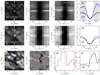 |
Fig. 2. Details of a QSEB in Hβ and Hα. (a) QSEB observed in the Hβ red wing. (b) Spatial variations in the Hβ line profile along the y-axis crossing the QSEB and shown by the two vertical white lines in (a). Here the spectral dimension is presented in terms of Doppler offset. (c) Temporal variations in the Hβ line profile for a location in the QSEB indicated by the blue plus sign in (a). (d) Hβ line profile at the brightest pixel in the QSEB and an average quiet Sun reference profile (black line). (e–h) Similar to (a–d), but in Hα. (i) Corresponding WB image, and (j) Map of BLOS. (k) Evolution of the BLOS flux (ϕ) within the red box shown in (j). (l) Light curves of the intensity variations of the QSEB (solid) and averaged over the FOV presented in this figure (dotted). Both the curves are averages of intensities in the Hβ line wings (Iw) as marked by the gray shaded area in (d). An animation showing evolution of the QSEB is available online. |
Figure 3 presents a QSEB event that is smaller, less bright, and shorter-lived than the QSEB in Fig. 2. The Hβ spectra show weak enhancement of the line wings, found in only six pixels, which indicates a QSEB area of around 8000 km2. On the other hand, the QSEB presented in Fig. 2 is approximately five times bigger. In the Hα observations the QSEB is hardly distinguishable from the background. The QSEB is among the shortest-lived QSEBs with a lifetime of ∼35 s, which is evident from the light curve of the QSEB and average background intensity plotted in Fig. 3l. Furthermore, the temporal evolution of the Hβ line profile in the QSEB shows the enhancement above the averaged background profile in four time steps; see the animation in Fig. 3. This QSEB also appears in an intergranular lane and has a very weak magnetic field strength (BLOS < 10 G). Two more QSEB examples are shown in Appendix B in the same format as Figs. 2 and 3.
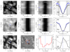 |
Fig. 3. Example QSEB that is small, short-lived, and less bright than the QSEB example in Fig. 2, but with the same format. An animation of this figure is available online. |
3.3. Hβ line core brightening associated with QSEBs
As mentioned before, the typical characteristics of EBs and QSEBs are the enhanced Hα wings and unaltered line core. The Hβ observations presented in this Letter show overwhelming evidence that the QSEB brightening also persists in the Hβ line core. In this section and Appendix C, we provide a few examples of the Hβ line core brightening associated with QSEBs.
Figure 4 shows the temporal evolution of a QSEB at different line positions in the Hβ line. At first, the QSEB appears in the line wings (at Doppler offsets of 41−55 km s−1), while it is barely visible in the intensity maps of the line flanks (14−27 km s−1) and absent in the line core. As the evolution of the QSEB progresses, the brightening appears in the line flanks and finally in the line core, approximately 50 to 80 s after the QSEB onset. By the time the brightening begins to appear in the line core, it weakens in the wings. Apart from its gradual progression to the line core from the wings, the QSEB also shows a systematic spatial displacement between the line wings and line core. The QSEB brightening in the line core is located more toward the limbward direction as compared to that in the wings; this indicates temperature enhancement at higher altitude. We note that not all QSEBs exhibit brightening in Hβ line core; only ∼400 out of 2800 QSEBs show the line core brightening in our dataset. Two additional examples of the QSEB brightening in the Hβ line core are discussed in Appendix C.
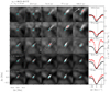 |
Fig. 4. Temporal evolution of a QSEB. Time progresses along the rows of Hβ images from left to right; the Doppler offset varies along the columns from the line core at the top to the far wing at the bottom. The rightmost column shows the evolution of the QSEB Hβ line profiles in red (the location of the line profile is given by the red plus sign in the images); the black line is a reference profile averaged over the presented FOV. The vertical dotted line gives the Doppler offset in the corresponding row. The Hβ profile is selected from the location of maximum intensity at that Doppler offset within the area of the QSEB. The cyan plus sign in each panel indicates the centre of the FOV. The dotted rectangle (center panel) shows the area used to create the space-time map displayed in Fig. 5b. |
We show space-time maps in Fig. 5 for the QSEBs displayed in Figs. 4, C.1, and C.2, which provide clear illustration of the gradual shift in the QSEB brightening from the Hβ line wings toward the line core as well as the gradual spatial displacement. From the diagonal slope in the space-time maps we estimate that the QSEB brightening moves from the line wings toward the line core with apparent velocities in the range 3−10 km s−1.
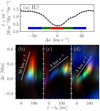 |
Fig. 5. Space-time maps demonstrating progression of the QSEB brightening from the Hβ line wings to the line core in time and space. The space-time maps in panels b–d are constructed as RGB color images with the Hβ line core image in the red channel, flanks in the green, and wings in the blue. The space-time maps in panels b–d correspond to the QSEBs presented in Figs. 4, C.1, and C.2, respectively. The displayed space-time maps are created by averaging intensities along the width of the dotted rectangle plotted in the central image of the respective figures, and Δr representing the length of the rectangles. The white lines in panels b–d indicate the apparent speed by which the QSEB brightening progresses from the wings to the core in the Hβ line. |
4. Discussion and conclusions
We present Hβ observations that reveal the ubiquitous presence of QSEBs in the quiet Sun. In the highest-quality images, recorded during the best seeing conditions, we find up to 120 QSEBs in uniform distribution over the FOV. This number of QSEBs is more than an order of magnitude higher than in the Hα observations of Rouppe van der Voort et al. (2016) who found fewer than ten QSEBs in their best images. We estimate that about half a million QSEBs could be present in the lower solar atmosphere at any given time. The QSEBs mainly arise in the intergranular lanes, but occasionally they also appear co-spatially with photospheric magnetic BPs. We find significant variation in QSEB properties ranging from larger (∼40 000 km2) and brighter QSEBs that last for several minutes to smaller (∼8000 km2) and less bright QSEBs that have a lifetime of a few tens of seconds. Comparing co-temporal Hα and Hβ observations, we conclude that the latter diagnostic is more suited to study QSEBs. QSEBs show more pronounced intensity enhancement of the Hβ wings, and small and weak QSEBs are difficult to distinguish from the background in the Hα observations. We attribute the unambiguous identification of QSEBs in Hβ observations to higher spatial resolution that can be achieved at shorter wavelengths. Another major factor is the intrinsic higher intensity contrast at shorter wavelengths where the Planck function has greater variation for different temperatures. The wings of hydrogen Balmer lines form in the lower parts of the solar atmosphere and are more coupled to the local thermodynamic conditions. Therefore, a temperature increase due to magnetic reconnection will result in a higher intensity enhancement of the Hβ line wings compared to the Hα line.
By definition, the quiet Sun is where the Sun exhibits minimal solar activity, and no large-scale magnetic flux emergence occurs. On the other hand, new magnetic flux does appear in the interior of supergranular cells (see Thornton & Parnell 2011; Gošić et al. 2016; Smitha et al. 2017, and references therein); Smitha et al. (2017) found the flux emergence rate of 1100 Mx cm−2 day−1. Moreover, with time, a significant fraction of newly appeared magnetic elements dissipate by cancellation with opposite polarity patches (Gošić et al. 2016; Smitha et al. 2017). So, flux cancellation prevails throughout the quiet Sun photosphere and might be responsible for QSEBs. We found episodes of flux cancellation in the photosphere that spatially and temporally coincide with QSEBs. This supports the idea that magnetic reconnection in the photosphere is the fundamental mechanism for QSEBs (Rouppe van der Voort et al. 2016; Shetye et al. 2018). Nonetheless, not all the QSEBs show flux cancellation in our data, and many appear with unipolar BLOS patches. We note that lower spatial and temporal resolution in our BLOS maps compared to the Hβ observations make it difficult to detect weak and small opposite polarity patches. Furthermore, projection effects in our off-center observations may hide magnetic patches rooted in deep intergranular lanes.
The three-dimensional (3D) radiation magnetohydrodynamic (MHD) simulations by Hansteen et al. (2017, 2019) successfully reproduce observable properties of EBs and suggest that they originate through magnetic reconnection in vertical or nearly vertical elongated current sheets in the lower solar atmosphere. In particular, Hansteen et al. (2019) explain the co-spatial and temporal presence of EBs and UV bursts (Peter et al. 2014) observed by Vissers et al. (2015), Tian et al. (2016), and Ortiz et al. (2020). Their simulations show that the reconnection in the upper part of the current sheet (in the chromosphere/transition region) produces enhanced Si IV emission associated with UV bursts, whereas EBs with enhanced Balmer wings occur in the lower part of the current sheet in the photosphere. Indications of a spatial offset between EBs and UV bursts in off-center observations were first found by Vissers et al. (2015) and later clearly demonstrated by Chen et al. (2019). Our observations of a flame-like morphology of QSEBs aligned along the limbward direction, and the associated brightenings in the Hβ line core that appear with a spatial offset toward the limb, indicate that QSEBs also originate in vertically elongated current sheets stretching between the photosphere and chromosphere. Moreover, the temporal delay in the Hβ line core brightening compared to the wings suggest progression of the magnetic reconnection from the photosphere toward the chromosphere with a speed of 3−10 km s−1.
In the flux emergence simulations by Hansteen et al. (2017, 2019), the magnetic reconnection responsible for EBs takes place in a ∪-shaped magnetic field topology, where the two opposite sides are advected through a converging photospheric flow, a scenario put forward by Watanabe et al. (2008), among others. On the contrary, Danilovic (2017) found the magnetic reconnection in Ω-shaped topology producing EBs in her 3D MHD simulations. Given the ubiquity of QSEBs and the minimal magnetic activity in the quiet Sun, it is less likely that QSEBs also originate in the magnetic field topology described above, which usually features in regions of large-scale flux emergence. Therefore, we propose an alternative scenario for QSEBs: mixed polarity magnetic patches in intergranular lanes produced by the local dynamo action (Petrovay & Szakaly 1993; Cattaneo 1999; Vögler & Schüssler 2007) might generate small-scale current sheets, and consequently magnetic reconnection. However, the proposed mechanism requires scrutiny through 3D numerical simulations.
A series of recent numerical studies (Priest et al. 2018; Syntelis et al. 2019; Syntelis & Priest 2020) suggest that ubiquitous photospheric flux cancellation driven by magnetic reconnection could act as a mechanism for chromospheric and coronal heating. Here we present the first ever unambiguous detection of ubiquitous magnetic reconnection in the lower solar atmosphere. In terms of ubiquity, this reminds one of the nanoflare mechanism of Parker (1988), a scenario of numerous and continuous small-scale reconnection events in the upper atmosphere that can explain coronal heating. It will be of great interest to quantify the energy budget of QSEBs and to explore their role in chromospheric and coronal heating.
Movies
Movie of Fig. 1 Access Supplementary Material
Movie of Fig. 2 Access Supplementary Material
Movie of Fig. 3 Access Supplementary Material
Movie of Fig. B.1. Access Supplementary Material
Movie of Fig. B.2 Access Supplementary Material
Acknowledgments
The Swedish 1-m Solar Telescope is operated on the island of La Palma by the Institute for Solar Physics of Stockholm University in the Spanish Observatorio del Roque de los Muchachos of the Instituto de Astrofísica de Canarias. The Institute for Solar Physics is supported by a grant for research infrastructures of national importance from the Swedish Research Council (registration number 2017-00625). This research is supported by the Research Council of Norway, project number 250810, and through its Centres of Excellence scheme, project number 262622. This study benefited from discussions during the workshop “Studying magnetic-field-regulated heating in the solar chromosphere” (team 399) at the International Space Science Institute (ISSI) in Switzerland. We made much use of NASA’s Astrophysics Data System Bibliographic Services. JdlCR is supported by grants from the Swedish Research Council (2015-03994), the Swedish National Space Agency (128/15). This project has received funding from the European Research Council (ERC) under the European Union’s Horizon 2020 research and innovation programme (SUNMAG, grant agreement 759548).
References
- Cattaneo, F. 1999, ApJ, 515, L39 [Google Scholar]
- Chen, Y., Tian, H., Peter, H., et al. 2019, ApJ, 875, L30 [NASA ADS] [CrossRef] [Google Scholar]
- Danilovic, S. 2017, A&A, 601, A122 [NASA ADS] [CrossRef] [EDP Sciences] [Google Scholar]
- de la Cruz Rodríguez, J. 2019, A&A, 631, A153 [NASA ADS] [CrossRef] [EDP Sciences] [Google Scholar]
- de la Cruz Rodríguez, J., Löfdahl, M. G., Sütterlin, P., Hillberg, T., & Rouppe van der Voort, L. 2015, A&A, 573, A40 [NASA ADS] [CrossRef] [EDP Sciences] [Google Scholar]
- Ellerman, F. 1917, ApJ, 46, 298 [NASA ADS] [CrossRef] [Google Scholar]
- Everitt, B. S. 1972, Br. J. Psychiatr., 120, 143 [Google Scholar]
- Gošić, M., Bellot Rubio, L. R., del Toro Iniesta, J. C., Orozco Suárez, D., & Katsukawa, Y. 2016, ApJ, 820, 35 [Google Scholar]
- Hansteen, V. H., Archontis, V., Pereira, T. M. D., et al. 2017, ApJ, 839, 22 [NASA ADS] [CrossRef] [Google Scholar]
- Hansteen, V., Ortiz, A., Archontis, V., et al. 2019, A&A, 626, A33 [NASA ADS] [CrossRef] [EDP Sciences] [Google Scholar]
- Libbrecht, T., Joshi, J., de la Cruz Rodríguez, J., Leenaarts, J., & Ramos, A. A. 2017, A&A, 598, A33 [NASA ADS] [CrossRef] [EDP Sciences] [Google Scholar]
- Löfdahl, M. G., Hillberg, T., de la Cruz Rodriguez, J., et al. 2018, ArXiv e-prints [arXiv:1804.03030] [Google Scholar]
- Nelson, C. J., Freij, N., Reid, A., et al. 2017, ApJ, 845, 16 [Google Scholar]
- Ortiz, A., Hansteen, V. H., Nóbrega-Siverio, D., & van der Voort, L. R. 2020, A&A, 633, A58 [CrossRef] [EDP Sciences] [Google Scholar]
- Parker, E. N. 1988, ApJ, 330, 474 [Google Scholar]
- Peter, H., Tian, H., Curdt, W., et al. 2014, Science, 346, 1255726 [Google Scholar]
- Petrovay, K., & Szakaly, G. 1993, A&A, 274, 543 [Google Scholar]
- Priest, E. R., Chitta, L. P., & Syntelis, P. 2018, ApJ, 862, L24 [Google Scholar]
- Rouppe van der Voort, L. H. M., Rutten, R. J., & Vissers, G. J. M. 2016, A&A, 592, A100 [NASA ADS] [CrossRef] [EDP Sciences] [Google Scholar]
- Rutten, R. J., Vissers, G. J. M., Rouppe van der Voort, L. H. M., Sütterlin, P., & Vitas, N. 2013, J. Phys. Conf. Ser., 440, 012007 [Google Scholar]
- Scharmer, G. B., Bjelksjö, K., Korhonen, T. K., Lindberg, B., & Petterson, B. 2003, in Innovative Telescopes and Instrumentation for Solar Astrophysics, eds. S. L. Keil, & S. V. Avakyan, Proc. SPIE, 4853, 341 [Google Scholar]
- Scharmer, G. B., Narayan, G., Hillberg, T., et al. 2008, ApJ, 689, L69 [Google Scholar]
- Scharmer, G. B., Löfdahl, M. G., Sliepen, G., & de la Cruz Rodríguez, J. 2019, A&A, 626, A55 [NASA ADS] [CrossRef] [EDP Sciences] [Google Scholar]
- Shetye, J., Shelyag, S., Reid, A. L., et al. 2018, MNRAS, 479, 3274 [Google Scholar]
- Smitha, H. N., Anusha, L. S., Solanki, S. K., & Riethmüller, T. L. 2017, ApJS, 229, 17 [Google Scholar]
- Syntelis, P., & Priest, E. R. 2020, ApJ, 891, 52 [NASA ADS] [CrossRef] [Google Scholar]
- Syntelis, P., Priest, E. R., & Chitta, L. P. 2019, ApJ, 872, 32 [NASA ADS] [CrossRef] [Google Scholar]
- Thornton, L. M., & Parnell, C. E. 2011, Sol. Phys., 269, 13 [Google Scholar]
- Tian, H., Xu, Z., He, J., & Madsen, C. 2016, ApJ, 824, 96 [CrossRef] [Google Scholar]
- van Noort, M., Rouppe van der Voort, L., & Löfdahl, M. G. 2005, Sol. Phys., 228, 191 [Google Scholar]
- Vissers, G. J. M., Rouppe van der Voort, L. H. M., & Rutten, R. J. 2013, ApJ, 774, 32 [NASA ADS] [CrossRef] [Google Scholar]
- Vissers, G. J. M., Rouppe van der Voort, L. H. M., Rutten, R. J., Carlsson, M., & De Pontieu, B. 2015, ApJ, 812, 11 [NASA ADS] [CrossRef] [Google Scholar]
- Vissers, G. J. M., Rouppe van der Voort, L. H. M., & Rutten, R. J. 2019, A&A, 626, A4 [NASA ADS] [CrossRef] [EDP Sciences] [Google Scholar]
- Vögler, A., & Schüssler, M. 2007, A&A, 465, L43 [NASA ADS] [CrossRef] [EDP Sciences] [Google Scholar]
- Watanabe, H., Kitai, R., Okamoto, K., et al. 2008, ApJ, 684, 736 [Google Scholar]
- Watanabe, H., Vissers, G., Kitai, R., Rouppe van der Voort, L., & Rutten, R. J. 2011, ApJ, 736, 71 [NASA ADS] [CrossRef] [Google Scholar]
Appendix A: Observations and data processing
CHROMIS sampled the Hβ spectral line at 4861 Å at 35 line positions between ±1.371 Å with 74 mÅ steps between ±1.184 Å. CHROMIS has a transmission profile FWHM of 100 mÅ at 4860 Å and a pixel scale of 0 038. With the CRISP instrument we observed the Hα, Fe I 6173 Å, and Ca II 8542 Å spectral lines. CRISP sampled the Hα line at 11 line positions between ±1.5 Å with 30 mÅ steps. We obtained the spectropolarimetric observation in the Fe I 6173 Å line sampled at 13 line positions with ±32 mÅ steps plus continuum at +680 mÅ.
High spatial resolution was achieved by the combination of good seeing conditions, the adaptive optics system, and the high-quality CRISP and CHROMIS reimaging systems (Scharmer et al. 2019). We also applied image restoration using the method of multi-object multi-frame blind deconvolution (MOMFBD; van Noort et al. 2005). The data was processed with the CRISP and CHROMIS data processing pipelines (de la Cruz Rodríguez et al. 2015; Löfdahl et al. 2018).
We performed Milne-Eddington inversions of the Fe I 6173 Å line data to infer the BLOS utilizing a parallel C++/Python implementation1 (de la Cruz Rodríguez 2019).
Appendix B: Additional QSEB examples
Two additional examples of QSEB are presented in Figs. B.1 and B.2. In terms of properties, the QSEB event displayed in Fig. B.1 is very similar to the QSEB in Fig. 2. The QSEB is located in intergranular lanes harboring multiple BLOS patches with mixed polarities, and the evolution of unsigned BLOS flux suggests a co-temporal flux cancellation episode.
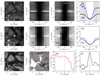 |
Fig. B.1. Another example of a QSEB in the same format as Fig. 2. An animation of this figure is available online. |
Finally, the QSEB shown in Fig. B.2 is an example of a QSEB that occurs on top of a photospheric magnetic BP (see panels a and i). Our dataset has many examples of QSEBs appearing co-spatially with photospheric magnetic BPs. A detailed analysis of lifetime, area, and brightness distribution of the QSEBs along with an analysis of the magnetic field topology will be presented in a follow-up paper.
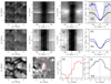 |
Fig. B.2. Example of a QSEB that appears co-spatially with a photospheric magnetic bright point. This figure is in the same format as Fig. 2. An animation of this figure is available online. |
Appendix C: Additional examples of the Hβ line core brightening
We show the temporal evolution of two QSEBs in the Hβ line in Figs. C.1 and C.2, in a manner similar to that in Fig. 4. These QSEBs present a scenario that is qualitatively similar to that described in Sect. 3.3: brightening in the Hβ line core with a temporal delay and spatial offset toward the limb compared to the QSEB brightening in the wings.
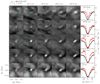 |
Fig. C.1. Another example of a QSEB that exhibits brightening in the Hβ line core. This figure is in the same format as Fig. 4. |
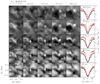 |
Fig. C.2. Example of a QSEB that is smaller and less bright than the QSEBs shown in Figs. 4 and C.1 and that exhibits brightening in the Hβ line core. This figure is in the same format as Fig. 4. |
Figure C.3 illustrates the temporal evolution of the same QSEB presented in Fig. 4, but in the Hα line instead of Hβ. Figure C.3 suggests that the QSEB also shows the progression from the wings to the flank in the Hα line. However, the QSEBs do not appear in the Hα line core, unlike the Hβ observations. The signature of the QSEB in the Hβ line core and its absence in the Hα line core suggest a difference in line core opacity of these two lines.
All Figures
|
Fig. 1. Ubiquitous QSEB detections using the k-means clustering technique. (a) Observed FOV in the Hβ blue wing. The red contours indicate the location of QSEBs. (b) Co-temporal continuum WB image. (c–f) Zoom-in on the four different areas indicated by the white boxes in (a); each panel shows duplicate images, one with the red contours indicating the location of QSEBs and one without the contours. The arrow in panel b shows the direction of the closest solar limb. An animation of this figure is available online. |
| In the text | |
|
Fig. 2. Details of a QSEB in Hβ and Hα. (a) QSEB observed in the Hβ red wing. (b) Spatial variations in the Hβ line profile along the y-axis crossing the QSEB and shown by the two vertical white lines in (a). Here the spectral dimension is presented in terms of Doppler offset. (c) Temporal variations in the Hβ line profile for a location in the QSEB indicated by the blue plus sign in (a). (d) Hβ line profile at the brightest pixel in the QSEB and an average quiet Sun reference profile (black line). (e–h) Similar to (a–d), but in Hα. (i) Corresponding WB image, and (j) Map of BLOS. (k) Evolution of the BLOS flux (ϕ) within the red box shown in (j). (l) Light curves of the intensity variations of the QSEB (solid) and averaged over the FOV presented in this figure (dotted). Both the curves are averages of intensities in the Hβ line wings (Iw) as marked by the gray shaded area in (d). An animation showing evolution of the QSEB is available online. |
| In the text | |
|
Fig. 3. Example QSEB that is small, short-lived, and less bright than the QSEB example in Fig. 2, but with the same format. An animation of this figure is available online. |
| In the text | |
|
Fig. 4. Temporal evolution of a QSEB. Time progresses along the rows of Hβ images from left to right; the Doppler offset varies along the columns from the line core at the top to the far wing at the bottom. The rightmost column shows the evolution of the QSEB Hβ line profiles in red (the location of the line profile is given by the red plus sign in the images); the black line is a reference profile averaged over the presented FOV. The vertical dotted line gives the Doppler offset in the corresponding row. The Hβ profile is selected from the location of maximum intensity at that Doppler offset within the area of the QSEB. The cyan plus sign in each panel indicates the centre of the FOV. The dotted rectangle (center panel) shows the area used to create the space-time map displayed in Fig. 5b. |
| In the text | |
|
Fig. 5. Space-time maps demonstrating progression of the QSEB brightening from the Hβ line wings to the line core in time and space. The space-time maps in panels b–d are constructed as RGB color images with the Hβ line core image in the red channel, flanks in the green, and wings in the blue. The space-time maps in panels b–d correspond to the QSEBs presented in Figs. 4, C.1, and C.2, respectively. The displayed space-time maps are created by averaging intensities along the width of the dotted rectangle plotted in the central image of the respective figures, and Δr representing the length of the rectangles. The white lines in panels b–d indicate the apparent speed by which the QSEB brightening progresses from the wings to the core in the Hβ line. |
| In the text | |
|
Fig. B.1. Another example of a QSEB in the same format as Fig. 2. An animation of this figure is available online. |
| In the text | |
|
Fig. B.2. Example of a QSEB that appears co-spatially with a photospheric magnetic bright point. This figure is in the same format as Fig. 2. An animation of this figure is available online. |
| In the text | |
|
Fig. C.1. Another example of a QSEB that exhibits brightening in the Hβ line core. This figure is in the same format as Fig. 4. |
| In the text | |
|
Fig. C.2. Example of a QSEB that is smaller and less bright than the QSEBs shown in Figs. 4 and C.1 and that exhibits brightening in the Hβ line core. This figure is in the same format as Fig. 4. |
| In the text | |
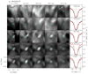 |
Fig. C.3. Same QSEB presented in Fig. 4, but for Hα observations instead of Hβ. |
| In the text | |
Current usage metrics show cumulative count of Article Views (full-text article views including HTML views, PDF and ePub downloads, according to the available data) and Abstracts Views on Vision4Press platform.
Data correspond to usage on the plateform after 2015. The current usage metrics is available 48-96 hours after online publication and is updated daily on week days.
Initial download of the metrics may take a while.