| Issue |
A&A
Volume 641, September 2020
|
|
|---|---|---|
| Article Number | A63 | |
| Number of page(s) | 7 | |
| Section | The Sun and the Heliosphere | |
| DOI | https://doi.org/10.1051/0004-6361/202038455 | |
| Published online | 10 September 2020 | |
Observational indications of magneto-optical effects in the scattering polarization wings of the Ca I 4227 Å line
1
Istituto Ricerche Solari Locarno, 6605 Locarno Monti, Switzerland
e-mail: emilia.capozzi@irsol.ch
2
Geneva Observatory, University of Geneva, 1290 Sauverny, Switzerland
3
Leibniz-Institut für Sonnenphysik (KIS), 79104 Freiburg, Germany
Received:
20
May
2020
Accepted:
20
June
2020
Context. Several strong resonance lines, such as H I Ly-α, Mg II k, Ca II K, and Ca I 4227 Å, are characterized by deep and broad absorption profiles in the solar intensity spectrum. These resonance lines show conspicuous linear scattering polarization signals when observed in quiet regions close to the solar limb. Such signals show a characteristic triplet-peak structure with a sharp peak in the line core and extended wing lobes. The line core peak is sensitive to the presence of magnetic fields through the Hanle effect, which however is known not to operate in the line wings. Recent theoretical studies indicate that, contrary to what was previously believed, the wing linear polarization signals are also sensitive to the magnetic field through magneto-optical (MO) effects.
Aims. We search for observational indications of this recently discovered physical mechanism in the scattering polarization wings of the Ca I 4227 Å line.
Methods. We performed a series of spectropolarimetric observations of this line using the Zurich IMaging POLarimeter camera at the Gregory-Coudé telescope at Istituto Ricerche Solari Locarno in Switzerland and at the GREGOR telescope in Tenerife (Spain).
Results. Spatial variations of the total linear polarization degree and linear polarization angle are clearly appreciable in the wings of the observed line. We provide a detailed discussion of our observational results, showing that the detected variations always take place in regions in which longitudinal magnetic fields are present, thus supporting the theoretical prediction that they are produced by MO effects.
Key words: polarization / scattering / Sun: chromosphere / Sun: photosphere / Sun: magnetic fields / techniques: polarimetric
© ESO 2020
1. Introduction
Over a decade ago, unexpected observations of the scattering polarization signal of the Ca I 4227 Å line were reported (see Bianda et al. 2003). This signal shows a triplet-peak structure with a sharp peak in the line core and broad lobes in the wings. The wing lobes, which are typical of strong resonance lines, are produced by coherent scattering processes. The observations of Bianda et al. (2003) were unexpected because, in addition to spatial variations in the Stokes Q/I wing signal (the reference direction for positive Q being the parallel to the closest limb), U/I wing signals of substantial amplitude showing similar spatial variations were found. Spatial variations of the Q/I wing lobes could, in principle, be explained in terms of variations of the anisotropy of the radiation field or variations of properties of the atmospheric plasma such as the density of neutral perturbers, which determine the fraction of coherent scattering processes. However, no straightforward physical explanation was readily available for the appearance and variation of U/I wing signals.
The observation of U/I signals in the line wings could not be explained in terms of the Hanle effect, as it is known to operate in the core of spectral lines and not in the wings (for an exhaustive overview, see Stenflo 1982; Trujillo Bueno et al. 2001; Landi Degl’Innocenti & Landolfi 2004). This circumstance led to the common belief that the large wing scattering polarization signals shown by strong resonance lines were insensitive to the presence of magnetic fields. On the other hand, Bianda et al. (2003) reported that the observed variations in the Q/I and U/I wings of the Ca I 4227 Å line were always accompanied by Zeeman signals in the nearby blends, thus suggesting that such unexpected wing behavior could indeed have a not yet understood magnetic origin. Sampoorna et al. (2009) investigated the possibility that the Hanle effect could extend in the wings, when a high rate of collisions and strong magnetic fields are present. However, these authors ruled out this explanation when considering realistic collisional rates and field strengths. We finally observe that at the spatial and temporal resolutions of the observations of Bianda et al. (2003) it can be excluded that the detected U/I signals could be produced by horizontal inhomogeneities in the solar plasma.
Theoretical investigations carried out in the last few years (see del Pino Alemán et al. 2016; Alsina Ballester et al. 2016) have shown that, in contrast to what was previously thought, the conspicuous scattering polarization signals observed in the wings of many strong resonance lines should be sensitive to the presence of magnetic fields. This sensitivity arises when longitudinal magnetic fields are present owing to the so-called magneto-optical (MO) effects. These effects most notably induce a rotation of the plane of linear polarization (often referred to as Faraday rotation; e.g., Pershan 1967), modifying the Q/I wing signal and giving rise to an appreciable wing signal in U/I. These MO effects have been theoretically predicted to have an appreciable impact on the scattering polarization wings of a number of strong resonance lines, including the Mg II k and h lines (del Pino Alemán et al. 2016; Alsina Ballester et al. 2016), the Sr II line at 4078 Å (Alsina Ballester et al. 2017), the H I Ly-α line (Alsina Ballester et al. 2019), and the Ca I line (Alsina Ballester et al. 2018). These theoretical investigations suggest MO effects as an ideal candidate for explaining observations such as those of Bianda et al. (2003). Moreover, these observations could offer a novel window into the magnetism of the solar atmosphere, providing complementary information to that accessible through the Hanle and Zeeman effects.
In this work we present new spectropolarimetric observations of the Ca I 4227 Å line carried out in regions with different levels of magnetic activity. We provide indications that variations of the Q/I wing lobes, together with the appearance of significant U/I wing signals, are observed in regions in which relatively strong longitudinal fields are present, thus supporting the theoretical prediction that such variations are produced by MO effects. In Sect. 2 we analyze the scattering polarization signal of the Ca I 4227 Å line, and we introduce the main physical quantities on which we base our analysis. In Sects. 3–5 we present our spectropolarimetric observations, which were carried out with the Zurich Imaging Polarimeter (ZIMPOL), both at GREGOR and at Istituto Ricerche Solari Locarno (IRSOL). For each of these, we briefly describe the instrumental setup, we provide information on the observed solar region, and we describe the data reduction procedure. Finally, we analyze the data, and we provide our conclusions.
2. Scattering polarization signal of the Ca I 4227 Å line
In the solar intensity spectrum, the Ca I 4227 Å line is characterized by a broad absorption profile with extended wings (see the upper panel of Fig. 1). It is produced by a resonance transition between the ground level of neutral calcium, which has total angular momentum Jℓ = 0 [1S0], and an upper level with Ju = 1 [1P ]. The line-core radiation originates primarily from atmospheric heights around 1000 km above the τ = 1 surface, making it chromospheric in nature (Supriya et al. 2014), while the radiation at wavelengths immediately outside the core of the line originates from photospheric heights, as illustrated in Fig. 2.
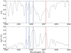 |
Fig. 1. Intensity spectrum (upper panel) and second solar spectrum (lower panel) across a wavelength interval containing the Ca I 4227 Å line (data from Gandorfer 2002). The blue and red lines indicate the wavelength intervals of interest for this work (see text). |
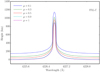 |
Fig. 2. Height at which the optical depth is unity as a function of wavelength across the Ca I 4227 Å line, in the semiempirical atmospheric model C of Fontenla et al. (1993), for various lines of sight (see legend). These curves provide a rough estimate of the formation region of the line as a function of wavelength. |
This line exhibits the largest scattering polarization signal in the visible range of the so-called second solar spectrum (Brückner 1963; Stenflo et al. 1980, 1984; Gandorfer 2002). The Q/I profile is characterized by a sharp peak in the line core and prominent lobes in the wings (see the lower panel of Fig. 1). This characteristic triplet-peak structure is typical of strong resonance lines. The Q/I wing lobes arise as a consequence of frequency coherent scattering processes (Holzreuter et al. 2005). As such, it can be shown that their amplitude is insensitive to the depolarizing effect of elastic collisions with neutral perturbers. On the other hand, elastic collisions may modify the amplitude of the scattering polarization wings through the branching ratios determining the fraction of coherent and noncoherent scattering processes (see Alsina Ballester et al. 2018). The drops in amplitude that can be observed within the wing lobes of the Q/I signal result from the presence of several blended lines, especially of Fe I, which can also be clearly observed in the intensity spectrum.
In this work we search for observational evidence of the theoretically predicted sensitivity of the scattering polarization wing lobes of the Ca I 4227 Å line to MO effects by comparing the spatial variations of the linear polarization signals to the magnetic activity within the same regions. To this aim, we analyzed the linear polarization angle (i.e., the angle between the direction of linear polarization and the specified reference direction) and the total linear polarization fraction at particular wing wavelengths. The polarization angle, which is defined within the interval [0° ,180° ) (e.g., Landi Degl’Innocenti & Landolfi 2004), is given by
According to this definition, when U/I = 0, α = 0° if Q/I > 0 and α = 90° if Q/I < 0, while when Q/I = 0, α = 45° if U/I > 0, and α = 135° if U/I < 0. The linear polarization angle is of course undefined when Q = U = 0. The total linear polarization fraction is given by
We note that the total linear polarization fraction of scattering polarization signals depends directly on the degree of anisotropy of the scattered radiation field.
The MO effects operating in the presence of a magnetic field with a longitudinal component produce a rotation of the plane of linear polarization, giving rise to a non-zero α angle. On the other hand, we may, in principle, expect such MO effects to preserve the polarization fraction PL. However, it should be noted that the emerging radiation is generally emitted over an extended region in the solar atmosphere. Since the rotation of the plane of linear polarization depends on the distance traveled through the medium, radiation emitted at different points is rotated by different amounts. As a consequence, the total linear polarization fraction of the radiation can decrease (see the Appendix A in Alsina Ballester et al. 2018).
In order to reduce the influence of blends as much as possible, we focus our attention on the wing wavelengths at which the Q/I signal shows local maxima (peaks). We consider four different wavelengths. Three are located in the blue wing; moving from the core to the wing, these are referred to as bI, bII, and bIII. The fourth is located in the red wing (hereafter referred to as rI). Because of the noise affecting the observed profiles, the position of the Q/I peaks is determined by performing a Gaussian fit of the observed signal around the considered peak and by finding the maximum of the ensuing curve. To minimize the noise in the analyzed physical quantities (α and PL), the observed signal is averaged over a small spectral interval centered at the fit maximum. The width of this interval must be large enough to reach an acceptable signal-to-noise ratio, but sufficiently narrow to not include spectral regions affected by the blends. We found a width of 50 mÅ to be suitable. We verified that the values of α and PL do not change appreciably if this value is slightly modified. Taking the observation of Gandorfer (2002) as reference, the wing intervals, determined as described above, are shown in Fig. 1. Such wing intervals can be specified through their distance from the line center, determined by finding the intensity absorption profile minimum, following a fitting procedure fully analogous to that previously described. In all the observations considered in this work, the wavelength intervals of interest are determined from the Q/I profiles averaged over the entire slit, following the aforementioned workflow.
3. Zeeman V/I signal in the nearby Fe I 4224.2 Å line
For the purpose of determining the magnetic origin of the spatial variations of the wing scattering polarization of the Ca I 4227 Å line, we analyzed the circular polarization signal produced by the Zeeman effect in the nearby Fe I 4224.2 Å line. Although it must be acknowledged that, in general, Stokes V is not strictly proportional to the longitudinal component of the magnetic field (see del Toro Iniesta & Ruiz Cobo 2016), it nevertheless provides a reliable indication of the level of magnetic activity of the observed region. For all the measurements presented in the following sections, we considered the maximum amplitude of the blue peak of the V/I signal of the aforementioned Fe I line, because the red peak is closer to another blended line.
4. Observations at GREGOR
The first observations that we analyzed were taken at the GREGOR telescope on June 24, 2018, using the ZIMPOL camera (see Ramelli et al. 2010), which was installed at the GREGOR spectrograph. The polarimeter analyzer, consisting of a double ferroelectric crystal (FLC) modulator followed by a linear polarizer, was mounted in front of the spectrograph slit after several folding mirrors; the FLC modulates the polarization signals at the frequency of 1 kHz, allowing us to “freeze” intensity variations due to seeing (see Ramelli et al. 2014, for technical details).
The spectrograph slit covers a solar area of ∼0.3″ (width of the slit) times 47″ (length of the slit). The ZIMPOL images presented in this work have 140 pixels along the spatial direction and 1240 pixels along the spectral direction. According to the Nyquist criterion, the attainable spatial resolution is ∼0.6″, while the spectral resolution is of ∼10 mÅ.
The GREGOR polarimetric calibration unit (GPU; Hofmann et al. 2012) is mounted at the second focal point (F2) before any folding reflection to avoid any significant instrumental polarization produced by the mirrors. Owing to the presence of a pre-filter in the GPU that blocks the radiation at all wavelengths below a cutoff just above the Ca I line, the polarimetric calibration measurements were performed at around 4240 Å and not at the exact wavelength of the line. The polarimetric calibration, dark images, and flat field (obtained by moving the telescope randomly around disk center) were recorded within a few minutes of the observations (see Dhara et al. 2019, for more details).
We carried out two observations: one on an active region close to the west limb, and one on a quiet region at a diametrically opposed position at the east limb. The latter was carried out to have an observation in the quiet Sun to be compared to the observation in the active region. For scheduling reasons, the observations were carried out around noon, which is a comparatively unfavorable time because the althazimuthal system rotates quite fast. This introduced time-dependent instrumental polarization signals that could not be completely removed in the data reduction. Moreover, the seeing was rather poor (r0 < 4), but still good enough for the purpose of this work. The slit was placed parallel to the limb, choosing the positive direction for Stokes Q to be parallel to the slit direction. The tip-tilt of the adaptive optics (AO) system (Berkefeld et al. 2016) was used to keep the limb distance constant with an uncertainty of ∼0.5″. The data of the two observations were corrected using a flat-field image and a dark image, and a Fourier filter was also used to remove the periodic fringes originated by both electronics and optics. Furthermore, because the absolute value of the polarization cannot be determined with the instrumental setup used in this campaign, the Stokes profiles of the measurements were properly shifted along the polarization scale so that in the continuum Q/I matches the theoretical value (Gandorfer 2002), while U/I and V/I are zero.
For each Stokes parameter, the statistical error has been determined as follows. A slit portion of 20 pixels, corresponding to a magnetically uniform region, is selected. Then, at each frequency, the standard deviation is taken over the considered portion. The value of the standard deviation with the highest occurrence is taken as the statistical error for all frequency points. On the other hand, the statistical error associated with the linear polarization fraction and linear polarization angle is taken as the average absolute difference between such quantities, calculated from the experimental data at the all spatial positions, and a smooth function fitting their variation along the slit.
4.1. Analysis of a GREGOR observation on a quiet region
We observed a quiet Sun region close to the east limb, at a limb distance of ∼6″. The duration of the measurement was around 8 minutes (240 frames of 1 second exposure time each, with 1 second of lag between two consecutive frames). Figure 3 shows this measurement and the corresponding spatially averaged Stokes profiles. The statistical error was determined as described in Sect. 4. It is 0.09% for Stokes Q/I and V/I and 0.06% for Stokes U/I.
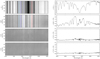 |
Fig. 3. Stokes I, Q/I, U/I, and V/I images (left) and spatially averaged profiles (right). The spatial average was performed over the entire slit. The intensity is normalized to the continuum. The observations were taken at ∼6″ from the solar limb, across a quiet region, with the slit oriented parallel to the nearest limb. The positive direction for Stokes Q is taken parallel to the limb. The wavelength intervals of interest are highlighted in the intensity and Q/I images. |
The Stokes Q/I profile shows the aforementioned triple peak structure, with a sharp peak at the line core and extended wing lobes; the highest polarization value in the blue lobe reaches ∼2%. We notice the persistence of some spurious effects in the U/I and V/I profiles, whose origin can be attributed to the fast changes of the instrumental polarization at the time of day at which the observation was taken (see Sect. 4). As discussed in Sect. 2, we focus our attention on four wavelength intervals in the wings, which are highlighted in Fig. 3 and whose distances from line center are given in Table 1.
The upper panel of Fig. 4 shows that the linear polarization angle is very close to zero along the whole slit for all the considered wavelengths. The anomalous peak found between 15″ and 17″ is of instrumental origin, resulting from dust grains in the optical system, close to the focal plane. This is supported by the bright horizontal stripe found at the same spatial position in Fig. 3. The total linear polarization fraction does not show any significant variation along the slit, at any of the considered wavelengths (see middle panel of Fig. 4). These results are compatible with our hypothesis because we are observing a quiet Sun region, where no magnetic fields capable of producing significant MO effects are expected. The absence of magnetic fields with a significant longitudinal component is confirmed by the very weak V/I signals observed in the nearby Fe I line (see lower panel of Fig. 4).
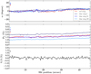 |
Fig. 4. Linear polarization angle (upper panel) and total linear polarization fraction (middle panel) along the slit for the considered wavelength intervals (see text and Table 1). In the lower panel, the amplitude of the blue peak of the V/I signal in the Fe I 4224.2 Å line is shown as a function of the slit position. The values shown in all three panels are obtained from the data presented in Fig. 3. The error bars (statistical error) are reported in the upper left part of each panel. |
4.2. Analysis of a GREGOR observation on an active region
At GREGOR, we also observed a region at 4″ from the west limb with modest magnetic activity, with part of the slit placed upon a region with moderate activity (see slit portion from ∼35″ to 47″ in Fig. 5). The duration of the measurement was around 9 minutes (284 frames of 1 second exposure time each, with 1 second of lag between two consecutive frames). The statistical error was determined as described in Sect. 4. It is 0.08% for Stokes Q/I and V/I and 0.07% for Stokes U/I.
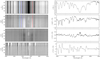 |
Fig. 5. Stokes I, Q/I, U/I, and V/I images (left) and spatially averaged profiles (right). The spatial average was performed over the slit positions from ∼35″ to 47″ (dashed line) where the magnetic field is strongest. The intensity is normalized to the continuum. The observations were taken at a limb distance of 4″, across a solar region with moderate magnetic activity, with the slit oriented parallel to the nearest limb. The positive direction for Stokes Q is taken parallel to the limb. The wavelength intervals of interest are highlighted in the intensity and Q/I images. |
Figure 5 shows the Stokes images and the corresponding spatially averaged profiles, for which the average was performed within the region where the magnetic field is strongest (i.e., over the slit portion from ∼35″ to 47″). In this region, Stokes Q/I again shows a triplet peak structure. However the line core peak, in comparison to the previous measurement (see Fig. 3), is clearly depolarized through the Hanle effect, which also induces significant U/I line-core signals. In the line wings prominent U/I signals are found along the entire slit. A significant depolarization of both Q/I and U/I wing signals is found in the region between ∼35″ and 47″. Indeed the blue wing maximum of the spatially averaged Q/I signal within this region is significantly smaller than in the previous measurement, which in this case is ∼0.7%. In the Stokes V/I and Q/I images, the typical patterns of the longitudinal and transverse Zeeman effect, respectively, can be observed.
The line-center distance of the wavelength intervals of interest for this observation, as defined in Sect. 2, are shown in Table 2. As can be seen in Fig. 6, the polarization angle differs appreciably from zero along the whole slit at all the considered wing wavelengths. This rotation of the plane of linear polarization is compatible with the impact of MO effects produced by a longitudinal magnetic field, whose presence is revealed by the Stokes V/I signal in the photospheric Fe I 4224.2 Å line. An increase of the amplitude of this V/I signal can be clearly observed between ∼35″ and 47″, confirming the presence of stronger longitudinal fields in this region (see the lower panel of Fig. 6). It is interesting to observe that while PL shows a clear decrease in this region, the variation of the polarization angle is less pronounced. This behavior can be interpreted observing that the anisotropy of the radiation field and other properties of the atmospheric plasma (e.g., the density of neutral perturbers) have a direct impact on PL, whereas they influence α only through its sensitivity to the magnetic field (Capozzi et al., in prep.). The observed variation of PL could thus be mainly ascribed to a variation of the properties of the atmospheric plasma in the region between ∼35″ and 47″, rather than to the presence of stronger fields via MO effects.
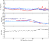 |
Fig. 6. Linear polarization angle (upper panel) and total linear polarization fraction (middle panel) along the slit for the considered wavelength intervals (see text and Table 2). In the lower panel, the amplitude of the blue peak of the V/I signal in the Fe I 4224.2 Å line is shown as a function of the slit position. The values shown in all three panels are obtained from the data presented in Fig. 5. The error bars (statistical error) are reported in the upper left of each panel. |
5. Observation at IRSOL and analysis
Another set of spectropolarimetric observations of the Ca I line at 4227 Å was performed with the ZIMPOL camera at IRSOL on April 19, 2019. The instrumental setup was similar to that used during the GREGOR campaign (Sect. 4), but the polarization modulation was done with a photoelastic modulator (PEM). This instrument modulates the signals with a frequency of 42 kHz, allowing us to minimize spurious effects induced by intensity variations due to the seeing.
The spectrograph slit covered a solar area of 0.5″ (width of the slit) times 180″ (length of the slit). Recalling that the ZIMPOL image has 140 pixels in the spatial direction and 1240 pixels in the spectral direction, the spatial sampling is ∼1.47″ pixel−1, and the spectral resolution is ∼10 mÅ. The polarimetric calibration, dark image, and flat-field image (obtained by moving the telescope randomly around disk center) were all recorded within few minutes of the observations. The data was corrected for flat-field and dark images, and a Fourier filter was used. Since the polarimetric calibration unit at IRSOL is mounted after two folding mirrors, some cross talk is unavoidable. The cross talk correction was made by performing a rotation around the U and Q axes of the Poincaré sphere until the V/I cross talk signal was minimized. In the observation that we analyzed, the cross talk from V/I to Q/I was corrected by a 6° rotation around the U axis, and the cross talk from V/I to U/I was corrected by a rotation around the Q axis with an angle of 5.5°.
Using a rotating glass tilt plate based on an elaboration of the slit jaw image, the distance of the limb to the spectrograph slit could be kept constant within an accuracy of ∼1″. Given the length of the slit of the IRSOL telescope, we also corrected for the effects of the curvature of the limb (Bianda et al. 2011).
We observed a region at 5″ from the west limb with moderate magnetic activity. The duration of the measurement was around 7 min (200 frames of 1 second exposure time each, with 1 second of lag between two consecutive frames). The slit was placed parallel to the nearest limb, and the reference direction for positive Stokes Q was chosen along the slit. The left panels of Fig. 7 show the Stokes images while the right panels show the corresponding profiles spatially averaged over the slit portion between ∼110″ and 170″ (i.e., over a region in which we have a strong magnetic field with a fixed polarity). The central peak of this Q/I profile is strongly depolarized through the Hanle effect. The maximum value of Q/I in the blue wing reaches ∼1% and prominent U/I signals are also found. In the region from ∼50″ to ∼170″, it is possible to recognize the typical patterns of the longitudinal Zeeman effect in the Stokes V/I image, as well as transverse Zeeman signals in Stokes Q/I and U/I. The statistical error was determined as described in Sect. 4. It is 0.09% for Stokes Q/I and 0.11% for Stokes U/I and V/I.
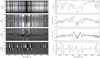 |
Fig. 7. Stokes I, Q/I, U/I, and V/I images (left) and spatially averaged profiles (right). The spatial average was performed over the slit positions from ∼110″ to 170″ (dashed line) where the magnetic field is strongest. The intensity is normalized to the continuum. The observation was taken at a limb distance of 5″, across a solar region with stronger magnetic activity, with the slit oriented parallel to the nearest limb. The positive direction for Stokes Q is taken parallel to the limb. The wavelength intervals of interest are highlighted in the intensity and Q/I images. |
In Fig. 8 the behavior of α, PL, and V/I along the slit is shown. The line-center distance of the wavelength intervals of interest considered in this observation, as defined in Sect. 2, are shown in Table 3.
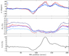 |
Fig. 8. Linear polarization angle (upper panel) and total linear polarization fraction (middle panel) along the slit for the considered wavelength intervals (see text and Table 3). In the lower panel, the amplitude of the blue peak of the V/I signal in the Fe I 4224.2 Å line is shown as a function of the slit position. These values are obtained from the data presented in Fig. 7. The error bars (statistical error) are reported in the upper left of each panel. |
Similarly to what is reported in Sect. 4.2, a clear change in the behavior of both PL and α can be noticed when going into the more magnetized region between ∼70″ and ∼170″. The behavior of α closely follows the variations of the V/I signal, including the change of sign in the region around 100″, strongly suggesting the impact of MO effects. On the other hand, PL is found to decrease sharply in this region, but it presents no clear variations within it. This could again be an indication that the total linear polarization fraction is mainly determined by the anisotropy of the radiation field and other nonmagnetic properties of the plasma (such as the rate of elastic collisions), which we may expect not to vary significantly within the magnetized region. Still focusing on the region around 100″, we may also propose an alternative explanation (compatible with the previous one). Within this region, we could expect the presence of magnetic fields of opposite polarities below the spatial resolution of the observation, leading to cancellations in both α and V/I (in agreement with their vanishing values found around 100″). It is an interesting consequence of MO effects that, if magnetic fields are present such that their orientation changes at scales below the resolution element but above the mean free path of the line’s photons, the magnetic fields would still contribute to depolarizing PL while at the same time cancellations would occur in α (see Appendix A in Alsina Ballester et al. 2018). Discriminating between these two scenarios is outside the scope of this work, but these observational results already provide tantalizing hints about the diagnostic potential of the MO effects.
6. Discussion and conclusions
In the present paper we have analyzed different spectropolarimetric observations of the Ca I 4227 Å line, obtained using the ZIMPOL camera with both the GREGOR and IRSOL telescopes. Spatial variations of the Q/I scattering polarization wing signals as well as the appearance of U/I wing signals, presenting similar spatial fluctuations, have been clearly detected. A comparison with the V/I signals produced by the Zeeman effect in the nearby Fe I 4224.2 Å line clearly indicates that such spatial variations are of magnetic origin, thus supporting the conclusion that they represent measurable signatures of MO effects operating on this line, as theoretically predicted in Alsina Ballester et al. (2018).
To make further advances in this line of investigation it will be of interest to have more quantitative information of the magnetic field present in the observed region. In this regard, the use of advanced spatially coherent inversion techniques (e.g., Asensio Ramos & de la Cruz Rodríguez 2015) will be highly beneficial in acquiring much needed information.
The results presented in this work also provide some hints regarding the potential of MO effects as a novel tool for magnetic field diagnostics, complementary to the Zeeman and Hanle effects. This motivates us to investigate the impact of MO effects on this line in greater depth. In a forthcoming publication, we will take a numerical approach, based on the solution of the non-LTE radiative transfer problem, to characterize the sensitivity of the four Stokes profiles of this line to magnetic fields, accounting for the joint action of the Hanle, Zeeman, and MO effects.
Acknowledgments
This research work was financed by the Swiss National Science Foundation (SNF) through grants 200020_169418 and 200020_184952. E.A.B. and L.B. gratefully acknowledge financial support by SNF through grants 200021_175997 and CRSII5_180238. IRSOL is supported by the Swiss Confederation (SEFRI), Canton Ticino, the city of Locarno and the local municipalities. The 1.5-meter GREGOR solar telescope was built by a German consortium under the leadership of the Kiepenheuer-Institut fur Sonnenphysik in Freiburg with the Leibniz-Institut für Astrophysik Potsdam, the Institut für Astrophysik Göttingen, and the Max-Planck-Institut für Sonnensystem forschung in Göttingen as partners, and with contributions by the Instituto de Astrofísica de Canarias and the Astronomical Institute of the Academy of Sciences of the Czech Republic.
References
- Alsina Ballester, E., Belluzzi, L., & Trujillo Bueno, J. 2016, ApJ, 831, L15 [Google Scholar]
- Alsina Ballester, E., Belluzzi, L., & Trujillo Bueno, J. 2017, ApJ, 836, 6 [Google Scholar]
- Alsina Ballester, E., Belluzzi, L., & Trujillo Bueno, J. 2018, ApJ, 854, 150 [Google Scholar]
- Alsina Ballester, E., Belluzzi, L., & Trujillo Bueno, J. 2019, ApJ, 880, 85 [Google Scholar]
- Asensio Ramos, A., & de la Cruz Rodríguez, J. 2015, A&A, 577, A140 [NASA ADS] [CrossRef] [EDP Sciences] [Google Scholar]
- Berkefeld, T., Schmidt, D., Soltau, D., Heidecke, F., & Fischer, A. 2016, in SPIE Conf. Ser., Proc. SPIE, 9909, 990924 [Google Scholar]
- Bianda, M., Stenflo, J. O., Gandorfer, A., et al. 2003, ASP Conf. Ser., 286, 61 [Google Scholar]
- Bianda, M., Ramelli, R., Stenflo, J. O., et al. 2011, ASP Conf. Ser., 437, 67 [Google Scholar]
- Brückner, G. 1963, Z. Astrophys., 58, 73 [Google Scholar]
- del Pino Alemán, T., Casini, R., & Manso Sainz, R. 2016, ApJ, 830, L24 [Google Scholar]
- del Toro Iniesta, J. C., & Ruiz Cobo, B. 2016, Liv. Rev. Sol. Phys., 13, 4 [Google Scholar]
- Dhara, S. K., Capozzi, E., Gisler, D., et al. 2019, A&A, 630, A67 [NASA ADS] [CrossRef] [EDP Sciences] [Google Scholar]
- Fontenla, J. M., Avrett, E. H., & Loeser, R. 1993, ApJ, 406, 319 [Google Scholar]
- Gandorfer, A. 2002, The Second Solar Spectrum: A high spectral resolution polarimetric survey of scattering polarization at the solar limb in graphical representation. Volume II: 3910 Å to 4630 Å (vdf ETH) [Google Scholar]
- Hofmann, A., Arlt, K., Balthasar, H., et al. 2012, AN, 333, 854 [Google Scholar]
- Holzreuter, R., Fluri, D. M., & Stenflo, J. O. 2005, A&A, 434, 713 [NASA ADS] [CrossRef] [EDP Sciences] [Google Scholar]
- Landi Degl’Innocenti, E., & Landolfi, M. 2004, Polarization in Spectral Lines (Dordrechet: Kluwer) [Google Scholar]
- Pershan, P. S. 1967, J. Appl. Phys., 38, 1482 [Google Scholar]
- Ramelli, R., Balemi, S., Bianda, M., et al. 2010, Proc. SPIE, 7735, 77351Y [Google Scholar]
- Ramelli, R., Gisler, D., Bianda, M., et al. 2014, in SPIE Conf. Ser., Proc. SPIE, 9147, 91473G [Google Scholar]
- Sampoorna, M., Stenflo, J. O., Nagendra, K. N., et al. 2009, ApJ, 699, 1650 [Google Scholar]
- Stenflo, J. O. 1982, Sol. Phys., 80, 209 [Google Scholar]
- Stenflo, J. O., Baur, T. G., & Elmore, D. F. 1980, A&A, 84, 60 [NASA ADS] [Google Scholar]
- Stenflo, J. O., Solanki, S., Harvey, J. W., & Brault, J. W. 1984, A&A, 131, 333 [NASA ADS] [Google Scholar]
- Supriya, H. D., Smitha, H. N., Nagendra, K. N., et al. 2014, ApJ, 793, 42 [Google Scholar]
- Trujillo Bueno, J. 2001, ASP Conf. Ser., 236, 161 [Google Scholar]
All Tables
All Figures
|
Fig. 1. Intensity spectrum (upper panel) and second solar spectrum (lower panel) across a wavelength interval containing the Ca I 4227 Å line (data from Gandorfer 2002). The blue and red lines indicate the wavelength intervals of interest for this work (see text). |
| In the text | |
|
Fig. 2. Height at which the optical depth is unity as a function of wavelength across the Ca I 4227 Å line, in the semiempirical atmospheric model C of Fontenla et al. (1993), for various lines of sight (see legend). These curves provide a rough estimate of the formation region of the line as a function of wavelength. |
| In the text | |
|
Fig. 3. Stokes I, Q/I, U/I, and V/I images (left) and spatially averaged profiles (right). The spatial average was performed over the entire slit. The intensity is normalized to the continuum. The observations were taken at ∼6″ from the solar limb, across a quiet region, with the slit oriented parallel to the nearest limb. The positive direction for Stokes Q is taken parallel to the limb. The wavelength intervals of interest are highlighted in the intensity and Q/I images. |
| In the text | |
|
Fig. 4. Linear polarization angle (upper panel) and total linear polarization fraction (middle panel) along the slit for the considered wavelength intervals (see text and Table 1). In the lower panel, the amplitude of the blue peak of the V/I signal in the Fe I 4224.2 Å line is shown as a function of the slit position. The values shown in all three panels are obtained from the data presented in Fig. 3. The error bars (statistical error) are reported in the upper left part of each panel. |
| In the text | |
|
Fig. 5. Stokes I, Q/I, U/I, and V/I images (left) and spatially averaged profiles (right). The spatial average was performed over the slit positions from ∼35″ to 47″ (dashed line) where the magnetic field is strongest. The intensity is normalized to the continuum. The observations were taken at a limb distance of 4″, across a solar region with moderate magnetic activity, with the slit oriented parallel to the nearest limb. The positive direction for Stokes Q is taken parallel to the limb. The wavelength intervals of interest are highlighted in the intensity and Q/I images. |
| In the text | |
|
Fig. 6. Linear polarization angle (upper panel) and total linear polarization fraction (middle panel) along the slit for the considered wavelength intervals (see text and Table 2). In the lower panel, the amplitude of the blue peak of the V/I signal in the Fe I 4224.2 Å line is shown as a function of the slit position. The values shown in all three panels are obtained from the data presented in Fig. 5. The error bars (statistical error) are reported in the upper left of each panel. |
| In the text | |
|
Fig. 7. Stokes I, Q/I, U/I, and V/I images (left) and spatially averaged profiles (right). The spatial average was performed over the slit positions from ∼110″ to 170″ (dashed line) where the magnetic field is strongest. The intensity is normalized to the continuum. The observation was taken at a limb distance of 5″, across a solar region with stronger magnetic activity, with the slit oriented parallel to the nearest limb. The positive direction for Stokes Q is taken parallel to the limb. The wavelength intervals of interest are highlighted in the intensity and Q/I images. |
| In the text | |
|
Fig. 8. Linear polarization angle (upper panel) and total linear polarization fraction (middle panel) along the slit for the considered wavelength intervals (see text and Table 3). In the lower panel, the amplitude of the blue peak of the V/I signal in the Fe I 4224.2 Å line is shown as a function of the slit position. These values are obtained from the data presented in Fig. 7. The error bars (statistical error) are reported in the upper left of each panel. |
| In the text | |
Current usage metrics show cumulative count of Article Views (full-text article views including HTML views, PDF and ePub downloads, according to the available data) and Abstracts Views on Vision4Press platform.
Data correspond to usage on the plateform after 2015. The current usage metrics is available 48-96 hours after online publication and is updated daily on week days.
Initial download of the metrics may take a while.