| Issue |
A&A
Volume 641, September 2020
|
|
|---|---|---|
| Article Number | A147 | |
| Number of page(s) | 12 | |
| Section | Extragalactic astronomy | |
| DOI | https://doi.org/10.1051/0004-6361/202038428 | |
| Published online | 23 September 2020 | |
γ-ray/infrared luminosity correlation of star-forming galaxies
1
Instituto Argentino de Radioastronomía (IAR, CCT La Plata, CONICET/CIC), C.C.5, (1984) Villa Elisa, Buenos Aires, Argentina
e-mail: paulakx@iar.unlp.edu.ar
2
Instituto de Astronomía y Física del Espacio, CONICET-UBA, C.C. 67, Suc. 28, 1428 Buenos Aires, Argentina
3
Institute for Nuclear Physics (IKP), Karlsruhe Institute of Technology (KIT), Karlsruhe, Germany
4
Instituto de Tecnologías en Detección y Astropartículas (CNEA, CONICET, UNSAM), Buenos Aires, Argentina
5
Universidad de Río Negro, Sede Atlántica – CONICET, Viedma CP8500, Río Negro, Argentina
Received:
15
May
2020
Accepted:
6
July
2020
Context. Nearly a dozen star-forming galaxies have been detected in γ-rays by the Fermi observatory in the last decade. A remarkable property of this sample is the quasi-linear relation between the γ-ray luminosity and the star formation rate, which was obtained assuming that the latter is well traced by the infrared luminosity of the galaxies. The non-linearity of this relation has not been fully explained yet.
Aims. We aim to determine the biases derived from the use of the infrared luminosity as a proxy for the star formation rate and to shed light on the more fundamental relation between the latter and the γ-ray luminosity. We expect to quantify and explain some trends observed in this relation.
Methods. We compiled a near-homogeneous set of distances, ultraviolet, optical, infrared, and γ-ray fluxes from the literature for all known γ-ray emitting, star-forming galaxies. From these data, we computed the infrared and γ-ray luminosities, and star formation rates. We determined the best-fitting relation between the latter two, and we describe the trend using simple, population-orientated models for cosmic-ray transport and cooling.
Results. We find that the γ-ray luminosity–star formation rate relation obtained from infrared luminosities is biased to shallower slopes. The actual relation is steeper than previous estimates, having a power-law index of 1.35 ± 0.05, in contrast to 1.23 ± 0.06.
Conclusions. The unbiased γ-ray luminosity–star formation rate relation can be explained at high star formation rates by assuming that the cosmic-ray cooling region is kiloparsec-sized and pervaded by mild to fast winds. Combined with previous results about the scaling of wind velocity with star formation rate, our work provides support to advection as the dominant cosmic-ray escape mechanism in galaxies with low star formation rates.
Key words: galaxies: starburst / galaxies: star formation / gamma rays: galaxies
© ESO 2020
1. Introduction
Among the γ-ray sources identified with extragalactic objects (e.g. Abdollahi et al. 2020), those associated with star-forming galaxies (SFGs) are of particular interest. Although the sample is still small, a clear correlation is observed between the γ-ray luminosity Lγ of these sources and observational tracers of the star formation rate (SFR) of their associated galaxies (mainly the infrared luminosity LIR; Ackermann et al. 2012; Tang et al. 2014; Rojas-Bravo & Araya 2016; Peng et al. 2016, 2019a; Griffin et al. 2016; Ajello et al. 2020). This correlation suggests that high-energy emission is produced mainly by stellar populations of SFGs, whereas any active galactic nucleus (AGN) eventually present would provide a minor contribution.
Star-forming galaxies have been observed by Fermi at gigaelectronvolt energies (Abdo et al. 2010a,b; Lenain et al. 2010; Ackermann et al. 2012); some SFGs have been observed by the Very Energetic Radiation Imaging Telescope Array System (VERITAS) and the High Energy Stereoscopic System (H.E.S.S.) at teraelectronvolt energies (Acciari et al. 2009; Acero et al. 2009). The sample comprises very different objects, including starburst galaxies (SBGs), ultraluminous IR galaxies (ULIRGs), and normal spirals such as M 31. Models predicting gigaelectronvolt to teraelectronvolt emission of SFGs had been developed before their detection (e.g. Völk et al. 1996; Blom et al. 1999; Romero & Torres 2003; Domingo-Santamaría & Torres 2005; Persic et al. 2008; de Cea del Pozo et al. 2009; Rephaeli et al. 2010). From the first observations, a consistent picture emerged (Persic et al. 2008; Rephaeli et al. 2010), in which gigaelectronvolt emission is dominated by hadronic interactions of cosmic rays (CRs) with interstellar protons. This process produces photons through neutral pion decay. As CRs are produced mainly by supernova remnants (SNRs, Jokipii & Morfill 1985; Bustard et al. 2017), high-SFR galaxies have higher CR energy densities, and therefore are more luminous in γ-rays (Persic & Rephaeli 2012). Alternative scenarios, in which galactic-scale super-winds accelerate CRs have also been proposed (Romero et al. 2018).
The fraction of the CR power that is lost to high-energy photons results from the interplay of CR cooling and escape mechanisms. Many works have been devoted to investigate their relevance in individual SFGs, with different levels of detail (Ackermann et al. 2012; Lacki & Thompson 2013; Yoast-Hull et al. 2014; Pfrommer et al. 2017; Wang & Fields 2018; Sudoh et al. 2018; Peretti et al. 2019). The results show that at high SFRs, galaxies behave as near-perfect calorimeters, radiating almost all the CR energy. Non-radiative processes would only be important at low SFRs, but their relative contribution is still controversial. Some authors (e.g. Peretti et al. 2020) propose that advection is the main non-radiative cooling mechanism down to very low SFRs, when diffusion overcomes it. Others (e.g. Pfrommer et al. 2017) claim that adiabatic cooling dominates the energy losses.
From the population standpoint, the most outstanding characteristic of the high-energy emission of SFGs is its correlation with SFR indicators. Using three-year Fermi data, Ackermann et al. (2012) found a quasi-linear correlation  for eight SFGs. The correlation spans more than four orders of magnitude in LIR, but their sample is rather small. Consequently, several works have improved the data set (Tang et al. 2014; Rojas-Bravo & Araya 2016; Peng et al. 2016, 2019a; Griffin et al. 2016). The most comprehensive work to date is that of Ajello et al. (2020), who compile a sample of 14 galaxies plus undetected objects from ten-year Fermi data, finding
  .
.
The investigation of the physics driving this correlation is important for several reasons. First, it allows us to understand the acceleration and evolution of CRs in galaxies (e.g. Wang & Fields 2018; Peretti et al. 2019). Second, a complete description of the correlation would allow us to accurately compute the contribution of SFGs to the extragalactic background γ-ray and neutrino fluxes (e.g. Sudoh et al. 2018; Peretti et al. 2020). Finally, escaped CRs, as well as high-energy photons, contribute to the energy feedback of SFGs into their surrounding medium. This contribution may have been important in the early Universe, when small SFGs were abundant and their energetic feedback influenced both the thermodynamic state of the intergalactic medium and the cosmic star formation history (e.g. Artale et al. 2015).
Some issues regarding the Lγ–SFR relation and its drivers, however, remain as yet poorly explored. A large effort has been devoted to improving γ-ray data, whereas little attention has been paid to the SFR. As noted by Pfrommer et al. (2017) and Zhang et al. (2019), the LIR–SFR relation relies on the assumption that most of the UV light emitted by massive stars is absorbed and re-radiated in the IR by dust. This is not true, for example, for low-metallicity SFGs such as the Small Magellanic Cloud (SMC). A thorough examination of this issue in the whole sample of γ-ray emitting SFGs, which is one of the aims of this work, is important to assess the validity of conclusions derived from the Lγ–LIR relation.
From the theoretical side, most previous works (Lacki & Thompson 2013; Sudoh et al. 2018; Peretti et al. 2019) focus on individual galaxies. These studies rely on multi-parameter models to fit the γ-ray spectra of SFGs. Each individual galaxy may require a different set of parameter values and, owing unavoidable correlations and degeneracies, it is difficult to extract a clear picture of which galaxy properties shape the Lγ–SFR relation from the combination of individual model results. A different insight is offered by population-orientated models (e.g. Zhang et al. 2019). These only rely on a few parameters that show scaling relations with the SFR (e.g. the Kennicutt-Schmidt or K-S law, Kennicutt 1998; Kennicutt & Evans 2012) and that influence the physical mechanisms driving CR behaviour. Usually, these works do not model in detail the CR particle distribution or γ-ray spectrum to obtain Lγ, computing instead the luminosity as an SFR-dependent fraction of the total CR energy. A third approach is proposed by Pfrommer et al. (2017), who use high-resolution, magneto-hydrodynamical (MHD) simulations to describe the formation and evolution of individual galaxies from gas in dark matter haloes, including CR injection, cooling, and escape. These MHD simulations can trace the physical mechanisms behind γ-ray emission, but the accuracy of their description of galaxies as a whole is limited by the sub-grid physics employed, especially that describing star formation.
In this paper, we combine the first two approaches, building a population-orientated model that treats the physical mechanisms responsible for γ-ray emission in detail. We improve upon previous models of this kind (e.g. Zhang et al. 2019) by including a full computation of the CR distribution and the γ-ray spectrum (similar to that of Peretti et al. 2019), while keeping the SFR scaling relations not present in individual-galaxy emission models. We carefully analyse the parameters and scaling relations needed to describe the regions of the galaxies in which high-energy radiation is emitted, and treat the rest of the parameters as fixed population means, or typical values.
This paper is organised as follows. In Sect. 2 we present SFR data taken from the literature for the full sample of SFGs observed up to date, plus the Milky Way (MW) and discuss the reliability of LIR as an SFR tracer in this sample. In Sect. 3 we develop our population-orientated model for γ-ray emission of SFGs, and compare it with previous models, paying special attention to the scaling relations that drive the Lγ–SFR correlation. In Sect. 4 we describe our results, which we discuss in Sect. 5, where we also present our conclusions.
2. Correlation of Lγ–SFR
In this section, we aim to revisit the Lγ–LIR relation, paying special attention to its lower end. We constructed the largest possible subsample of γ-ray emitting SFGs with near-homogeneous γ-ray, IR, and SFR data, and derived the more fundamental Lγ–SFR relation. The latter allowed us to quantify the biases introduced by the use of LIR as a proxy for the SFR in the whole range.
Previous works have compiled samples of LIR and Lγ published in the last 25 years. Improvements in extragalactic distance measurements in this period have produced changes in the accepted distances to many nearby galaxies, sometimes by large amounts (see e.g. the compilation of measurements in the NASA/IPAC Extragalactic Database; NED1). In some previous works, updated distance values were used to compute Lγ, whereas data on LIR were taken from literature sources that use outdated distances. We enforced the self consistency of our sample by only taking fluxes from γ-ray and IR catalogues, and computing luminosities using a single, near-homogeneous set of distances. Also, because SFRs are computed from fluxes (e.g. Kennicutt & Evans 2012), we always used the same set of distances described above to preserve the self-consistency of our sample. The self-consistent use of distances is crucial to obtain robust results. Table 1 compiles the estimates of Lγ, LIR, and Ṁ∗ (the SFR) for the 14 SFGs detected in γ-rays so far, plus the MW. In every case, we took care to compute reliable values of the uncertainties for all quantities to perform meaningful statistical analyses on our sample.
Distances, SFRs, IR, and γ-ray fluxes and luminosities for all γ-ray emitting SFGs known.
2.1. Distances
We adopted the best luminosity-distance value DL available for each galaxy to construct our set of distances. We took distances from the Cosmicflows-3 catalogue of Tully et al. (2016) when possible (nine objects). The estimates of these authors rely on redshift-independent methods (e.g. Tully-Fisher, Cepheids and red giant branch tip) therefore, to keep the homogeneity of our sample, for the remaining galaxies we searched in NED for measurements performed with similar methods that are compatible with the current cosmological model. This search failed in only three cases (NGC 3424, Arp 220, and Arp 299). For these we took the distances computed by NED using redshifts and Hubble flow modelling. As these are distant systems (> 25 Mpc), we expect redshift-dependent methods to provide reliable data.
The values obtained from the aforementioned sources are proper (metric) distances. For all but the three farthest galaxies in our sample, proper and luminosity distances coincide to better than 0.5%, therefore we take them to be identical. In the remaining cases, we computed luminosity distances from proper distances using the nine-year Wilkinson Microwave Anisotropy Probe (WMAP) cosmological model (Hinshaw et al. 2013).
2.2. Luminosities and SFRs
In previous works, the total IR luminosity LIR in the 8 − 1000 μm band is usually used as a proxy for the SFR. The quantity LIR can be computed from IRAS 12, 25, 60, and 100 μm fluxes using the formulae in Sanders & Mirabel (1996). We took the IRAS fluxes from the catalogues of Brauher et al. (2008, for Circinus) and Sanders et al. (2003, for all of the remaining galaxies except the MW), and derived both the FIR and LIR; we derived the latter using the luminosity distance described in Sect. 2.1. For the MW, we adopted the IR luminosity from Strong et al. (2010).
For all the galaxies in our sample, we computed their γ-ray luminosities using the observed flux in the 0.1 − 100 GeV band, and the luminosity distance to each one. For 11 galaxies we used the most recent data provided by the Fermi source catalogue (4FGL; Abdollahi et al. 2020). The γ-ray flux for the Large Magellanic Cloud (LMC) in the 4FGL is the result of the sum of the fluxes of 4 extended sources (4FGL J0500.9–6945e, 4FGL J0519.9–6845e, 4FGL J0530.0–6900e, and 4FGL J0531.8–6639e; Ackermann et al. 2016). Fluxes in the 0.1 − 100 GeV band are not reported in 4FGL for Arp 299, M 33, and NGC 2403, therefore we computed these from the 0.1 − 800 GeV energy fluxes and the best-fitting spectral energy distributions (SEDs) provided by Ajello et al. (2020). We also included the modelled γ-ray luminosity for the MW (Strong et al. 2010; Ackermann et al. 2012). It is important to stress that MW data were only added to perform qualitative comparisons because the MW is an important landmark for any study of SFGs. The MW data depend on models of CR propagation, γ-ray emission, and the IR interstellar radiation field. Their inclusion in the quantitative analysis would destroy the homogeneity of our data set, introducing biases that we cannot quantify.
As we aim to test the reliability of LIR as a proxy for the SFR within our sample, we avoided using the total IR luminosity in the determination of the SFR of our galaxies whenever possible. Far ultraviolet (FUV; λ ∼ 150 nm) and Hα fluxes are good tracers of SFR in unobscured systems, and several methods have been devised to include the effects of dust in obscured objects using multiwavelength (FUV+IR or Hα+IR) composite tracers (Kennicutt & Evans 2012). Among the latter, we chose those using monochromatic IR fluxes to keep our estimates independent of LIR. We compiled GALEX FUV fluxes (Gil de Paz et al. 2007; Cortese et al. 2012) and Hα fluxes (Kennicutt et al. 2008) for eight and nine galaxies, respectively. Five of these have estimates of both fluxes. We combined FUV and Hα fluxes with IRAS 25 μm fluxes from Sanders et al. (2003) and compiled distances to compute SFRs via the following formulae provided by Kennicutt & Evans (2012):
![$$ \begin{aligned}&\log \dot{M}_* [{M}_\odot \,\mathrm{yr}^{-1}] = \log (L_{\rm FUV} + 3.89 L_{25\,\mu \mathrm{m}}) [\mathrm{erg\,s}^{-1}] - 43.35;\end{aligned} $$](/articles/aa/full_html/2020/09/aa38428-20/aa38428-20-eq3.gif)
![$$ \begin{aligned}&\log \dot{M}_* [{M}_\odot \,\mathrm{yr}^{-1}] = \log (L_{\mathrm{H}\alpha } + 0.02 L_{25\,\mu \mathrm{m}}) [\mathrm{erg\,s}^{-1}] - 41.27. \end{aligned} $$](/articles/aa/full_html/2020/09/aa38428-20/aa38428-20-eq4.gif)
In these equations, LFUV and L25 μm are the monochromatic (νLν) luminosities at 150 nm and 25 μm, respectively, and LHα is the total luminosity in the Hα line. For the five galaxies with both FUV and Hα data, the two SFRs agree within measurement errors. We took the former values in the subsequent analysis.
For two galaxies (Arp 220 and Arp 299) we could not find any Hα or FUV measurement. These are IR-luminous systems with a large obscuration, for which LIR is expected to be the best SFR tracer. Therefore we computed their SFRs as
![$$ \begin{aligned} \dot{M}_*[{M}_\odot \,\mathrm{yr}^{-1}] = 1.7 \times 10^{-10} \epsilon \, L_{\rm IR} [{L}_\odot ], \end{aligned} $$](/articles/aa/full_html/2020/09/aa38428-20/aa38428-20-eq5.gif)
where ϵ depends on the initial mass function (IMF; Kennicutt 1998). As the FUV and optical tracers taken from Kennicutt & Evans (2012) are consistent with a Chabrier (2003) IMF, we adopted ϵ = 0.79 (Crain et al. 2010). Finally, following Kennicutt & Evans (2012), we took the SFR value of Chomiuk & Povich (2011) for the MW.
To assess the reliability of our SFR values, we compared these with (non-IR-based) measurements in the literature (Israel 1997; Wilke et al. 2004; Harris & Zaritsky 2004, 2009; For et al. 2012; Lanz et al. 2013; de los Reyes & Kennicutt 2019). We find that, once rescaled to our distances, published values agree well with ours within uncertainties. The only exception is NGC 3424, for which we find a 3.1σ difference between our SFR and that published by Lanz et al. (2013), where σ is the combined error of both measurements. Our value is higher by ∼0.9 M⊙ yr−1, similar to the offset they find between their SED-based and FUV-based SFRs. These authors explain this as an effect of the different SFR timescales probed by their method and FUV-based techniques. We conclude that our sample is well suited for the task of investigating the reliability of the Lγ–LIR correlation.
In the upper panel of Fig. 1 we show the correlation we find between the IR luminosity and SFR of the galaxies of our sample, whereas in the lower panel we plot the residuals Δ of the correlation, weighted by their standard deviation (computed from both LIR and Ṁ∗ uncertainties). As expected, luminous IR galaxies lie on the locus given by Eq. (3). For comparison, we plot the corresponding relation for both ϵ = 0.79 and 1 (the latter corresponds to the IMF of Salpeter 1955). For Ṁ∗ ≳ 1 M⊙ yr−1, most galaxies follow tightly the SFR–LIR correlation defined by Kennicutt & Evans (2012). Only NGC 3424 and NGC 4945 deviate from the relation, the former marginally (Δ = −2.1). The latter deserves some discussion because the strong downward deviation (Δ = −4.2) implies a higher IR emission than that expected from a complete conversion of UV photons into IR radiation by dust at the measured SFR value. Either NGC 4945 has a strong non-thermal source of IR radiation or the Hα+IR proxy used severely underestimates the SFR. The fact that this galaxy has a strong obscuration and is observed nearly edge-on (Strickland et al. 2004) favours the second explanation. However, multiwavelength observations would be required to completely settle this issue.
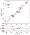 |
Fig. 1. Upper panel: SFR as a function of IR luminosity for our sample galaxies. The red dot-dashed and grey dashed lines represent the Ṁ∗(LIR) scaling relation presented in Eq. (3) for ϵ = 1 and 0.79, respectively. Lower panel: residuals of the Ṁ∗(LIR) relation for ϵ = 0.79, weighted by their standard deviation, as a function of LIR. The horizontal dotted lines correspond to ±3 standard deviations. |
For Ṁ∗ ≲ 1 M⊙ yr−1, galaxies deviate upwards from the linear relation of Eq. (3). Their SFRs are consistently higher than those predicted by IR luminosities; Δ > 3.6 in all cases but M 31. We interpret this as an effect of the incomplete obscuration of their star-forming regions, their IR luminosities accounting only for a fraction of their SFRs. This result suggests that LIR is not a reliable tracer for the low-SFR end of the sample of γ-ray emitting SFGs and that the Lγ–SFR correlation deserves further exploration.
In Fig. 2 (left panels) we present the variation of Lγ with LIR, constructed using the data in Table 1. A clear trend is seen, from which only NGC 3424 deviates significantly. The extreme γ-ray luminosity of this galaxy has already been noted by Ajello et al. (2020) and may be due to the presence of an AGN (Gavazzi et al. 2011), although this hypothesis has not yet been confirmed. A power-law fit ( ) to the remaining data results in m = 1.21 ± 0.07, log A = 27.47 ± 0.65, and a dispersion of 0.34 dex, indicating a relatively tight relation. The index m is consistent with that obtained by previous authors (Ackermann et al. 2012; Ajello et al. 2020). A linear behaviour (m = 1) can be rejected at the 3σ level.
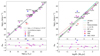 |
Fig. 2. Upper left panel: γ-ray luminosity of as a function of total IR luminosity for our sample. The grey solid line represents the best fit to the data (excluding the MW and NGC 3424) and the grey shaded region shows its 68% confidence level. The trend is consistent with those found by previous works. Lower left panel: residuals of the fit, weighted by their standard deviation, as a function of the total IR luminosity. The horizontal dotted lines correspond to ±3 standard deviations. Upper right panel: γ-ray luminosity as a function of SFR. Three fits performed on different data sets are shown: the full data set (cyan solid line); a reduced data set, excluding the MW and NGC 3424( green dashed line); and the BF, excluding all galaxies in the range −0.5 < log Ṁ∗ < 0.5 (grey dot-dashed line, see text). The grey shaded region shows the 68% confidence level of the BF fit. The red dotted line represents the best fit to the Lγ–LIR relation presented in the left panel, translated into the SFR–Lγ plane by Eq. (3), with ϵ = 0.79. The latter agrees only marginally with the data or any of the other three fits. Lower right panel: residuals of the BF fit, weighted by their standard deviation, as a function of the SFR. Horizontal dotted lines correspond to ±3 standard deviations. |
The right panels of Fig. 2 show the same correlation, but using our SFR instead of its IR tracer. A fit on the full data set (excluding the MW) gives an index m = 1.43 ± 0.15, log A = 39.32 ± 0.17, and a large dispersion of 0.65 dex, which is two times that of the Lγ–LIR correlation. Using a reduced data set (excluding NGC 3424 and the MW) we get m = 1.38 ± 0.12, log A = 39.22 ± 0.13, but with a smaller dispersion of 0.45 dex (still larger than that of the IR correlation). The large dispersion seems to be due to the data at intermediate SFRs (−0.5 ≲ log Ṁ∗ ≲ 0.5), therefore we try a third sample (called best followers; BF) excluding the five galaxies in this SFR range. A fit to this latter data set gives m = 1.35 ± 0.05, log A = 39.02 ± 0.07 and a dispersion of 0.21 dex, implying a much tighter relation. In all cases, a linear behaviour of Lγ with SFR can be rejected at least at the 2.8σ level. In the case of the BF correlation, the confidence level increases to almost 7σ.
To compare the IR and SFR correlations involving Lγ, we show in the upper left panel of Fig. 2 the best fit to the Lγ–LIR relation, translated into the SFR–Lγ plane by Eq. (3). Its index (m = 1.21 ± 0.05) is only marginally consistent with the BF index (m = 1.35 ± 0.05) at the 2σ level, where σ is the combined error of both indices. The IR correlation largely overestimates the γ-ray luminosity of low-SFR galaxies. This is consistent with our previous result that the IR luminosity underestimates the SFR. The IR relation index does not agree with those of the fits performed on the other two samples either, but these differences have a smaller significance.
To summarise, we showed that in our sample the IR luminosity consistently underestimates the SFR at low values. This makes the Lγ–LIR relation shallower than Lγ–SFR, the index of the former being lower by 0.14. In all cases, a linear relation between Lγ and either LIR or SFR is rejected with high confidence, at least 3σ. We also found a large dispersion in the latter at intermediate SFRs. In the next section, we devise models for γ-ray emission aimed at explaining the main features of the observed Lγ–SFR correlation.
3. Emission model
3.1. Cosmic-ray injection and density within galaxies
We aim to make progress in the understanding of the processes that shape the observed Lγ–SFR correlation (Ackermann et al. 2012) along the whole SFR range. This encompasses both quiescent SFGs, showing a low star formation activity spread on kiloparsec-scale discs, and the most active SBGs, with large SF activities concentrated in compact, sub-kiloparsec nuclei. The correlation connects two integrated properties of galaxies, and previous works (e.g. Ackermann et al. 2012; Zhang et al. 2019) suggest that it is possible to describe it based on the global CR energy balance. We thus choose a leaky-box model (Cowsik et al. 1967) to compute the CR populations in SFGs and their emission. Leaky-box are the simplest models available. They assume a homogeneous system in which CRs are injected at some rate, and of which CRs leak out in a finite time scale. These models do not capture the effects of gradients within SFGs, and they lack a detailed description of mechanisms such as diffusion or advection. The average effects of these mechanisms are parametrised by the leaking timescales. In spite of these shortcomings, leaky-box models can still capture the essentials of the CR energy balance (e.g. Peretti et al. 2019). We stress that our models do not try to fit the detailed emission of individual galaxies. Instead, we try to reproduce the mean Lγ of a typical galaxy, given its SFR and a few global properties that either correlate with SFR or are fixed (representing averages over the whole SFG population).
In our model, CRs of energy E are assumed to be injected within the galaxies at a steady rate Q(E), and cool and leak out of the CR cooling region in finite timescales τcool and τesc, respectively. The CR distribution within the region of the galaxy in which injection and cooling occurs is then

where i = e, p stands for electrons or protons and  . For the injection term Q(E) we adopt a power law with a quasi-exponential cutoff,
where the normalisation is Q0, i, maximum particle energy Emax, i, spectral index αi, and δp, e = (1, 2) (Zirakashvili & Aharonian 2007; Blasi 2010). We assume that CRs are accelerated in SNR shocks by the Fermi diffusive shock acceleration mechanism (Axford et al. 1977; Bell 1978; Blandford & Ostriker 1978), leading to αi = 2.2 for both protons and electrons (Lacki & Thompson 2013). According to Merten et al. (2017), plausible hadron-to-lepton ratios for SFGs are a = Q0, p/Q0, e > 10. At these large ratios, it is expected that hadrons dominate the emission, rendering the exact value of a irrelevant. We therefore adopt an intermediate value a = 50 in the following discussion. We verified a posteriori that different values of a > 10 do not change our results.
The total CR proton power injected by SNRs into the interstellar medium (ISM) of the galaxies is written as
where ξ = 0.1 is the injection efficiency, and ESN = 1051 erg is the typical energy released by a SN explosion. The supernova rate of the galaxy is ΓSN = (83 M⊙)−1 Ṁ∗, consistent with the Chabrier (2003) IMF adopted in this work (Ackermann et al. 2012). This provides the normalisation value of Q0, p, and gives the basic dependence of γ-ray emission on SFR.
In the presence of Bohm diffusion, as usually assumed for SNR environments, maximum particle energies can be obtained by the formulae given by Gaisser et al. (2016). For a typical shock velocity of vsh = 5000 km s−1 and a typical SNR magnetic field of BSNR = 200 μG, we obtain Emax, p ∼ 1 PeV and Emax, e ∼ 10 TeV. We also adopt Emin, p = 1.2 GeV and Emin, e = 1 MeV as minimum particle energies.
3.2. Cosmic-ray escape
Cosmic rays are advected by supernova-driven galactic winds (e.g. Strickland & Heckman 2009) and are diffuse in the ISM owing to their interaction with magnetic turbulence. Both processes lead to the escape of CRs from the galaxy at a rate  , where τdiff and τadv are the diffusion and advection characteristic timescales, respectively.
For τadv, we adopt the time that takes the wind to leave the CR cooling region (Persic & Rephaeli 2012),
where vw is the galactic wind velocity, and H the shortest size of the region (i.e. the disc height).
On the other hand, τdiff = H2/D(E), where D(E) is the diffusion coefficient, for which we explore two prescriptions representing extreme conditions for magnetic turbulence. For the first approach, we adopt a Kolmogorov diffusion coefficient with the normalisation found for our Galaxy, DK = 3.86 × 1028(E/GeV)1/3 cm2 s−1 by Berezinsky (1990), which leads to a fast diffusion. More recent estimates agree in order of magnitude with this value (see e.g. Gabici et al. 2019, and references therein). For the other case, we adopted a Bohm diffusion coefficient DB = Ec/(3eB), where B is the magnetic field of the ISM, e the electron charge, and c the speed of light. The recipes for determining the values of H, B, and vw are discussed in Sect. 3.4.
3.3. Cosmic-ray cooling and emission
Cooling of CRs proceeds by different mechanisms, each one contributing with a rate  to the total cooling rate as
The considered cooling mechanisms are synchrotron radiation, inverse Compton (IC) scattering, ionisation, and Bremsstrahlung for electrons, and inelastic p-p scattering and ionisation for protons. Their timescales can be expressed as (Ginzburg & Syrovatskii 1964; Blumenthal & Gould 1970; Lacki & Thompson 2013; Schlickeiser 2002; Kelner et al. 2006, and references therein),
where n is the ISM proton density (whose value is discussed in Sect. 3.4), and β = v/c with v the CR proton velocity. The cross section for inelastic p-p scattering is written as (Kelner et al. 2006)
![$$ \begin{aligned} \sigma _{\rm pp}(E) = (34.3 + 1.88 L + 0.25 L^2) \times \left[1-\left(\frac{E_{\rm th}}{E} \right)^4 \right]^2 \,\mathrm{mb}, \end{aligned} $$](/articles/aa/full_html/2020/09/aa38428-20/aa38428-20-eq20.gif)
where Eth = 1.22 × 10⁻³ TeV is the threshold energy for π0 meson production, L = ln(E/TeV) and κ = 0.5 is the in-elasticity of the process. Ionisation timescales assume a small fraction of ionised gas in the region where CRs propagate.
The main contribution to the photon field in the ISM is provided by cold dust that radiates in the IR, with a quasi-black-body spectrum (e.g. Draine 2011). Therefore, for the IC cooling time we use the parametrisation given by Khangulyan et al. (2014) for an isotropic, diluted (by a factor Σ), black-body radiation field of temperature T = 20 K,
where ℏ is the reduced Planck constant, r0 the classical electron radius, me the electron mass, and Fiso a dimensionless function of T and E. The value of Σ depends on the geometry of the system, and is discussed in Sect. 3.4.
The above formulae allow us to compute the particle distribution Np, e(E) predicted by our model. From these, we compute the SED of each emission process, using standard formulae for their emissivities (Blumenthal & Gould 1970; Kelner et al. 2006; Khangulyan et al. 2014). We obtain the total γ-ray luminosity in the Fermi energy range by integrating the SED between 0.1 and 100 GeV.
3.4. Parameters and scale relations
Our model has a single independent variable, the SFR, which defines the amount of CRs produced in each galaxy. This is linear in the SFR, therefore the non-linearity of the observed Lγ–SFR relation must arise from other SFR-dependent parameters. The most obvious candidate is the ISM proton density, as a large body of work has documented the existence of a correlation between the surface densities of SFR (ΣSFR) and cold gas mass (Σgas) of galaxies (the K-S law; Kennicutt 1998; Kennicutt & Evans 2012; de los Reyes & Kennicutt 2019), that is
![$$ \begin{aligned} \log {\Sigma _{\rm SFR}}\,[{M}_\odot \,\mathrm{yr}^{-1}\,\mathrm{kpc}^{-2}] = 1.41 \log {\Sigma _{\rm gas}}\,[{M}_\odot \,\mathrm{pc}^{-2}] - 3.74. \end{aligned} $$](/articles/aa/full_html/2020/09/aa38428-20/aa38428-20-eq22.gif)
We include the K-S law in our model to compute the density of protons n. As the K-S law relates intensive quantities, we are forced to take into account the geometry of the CR acceleration and cooling region. Most SFGs and SBGs show flattened morphologies, therefore we model this region as a disc of radius R and thickness 2H. The proton density is then
We stress that this disc models the region in which CRs cool, which needs not be the whole galaxy. de los Reyes & Kennicutt (2019) find that star-forming regions in disc galaxies, defined by Hα emission, are confined to smaller radii (by a factor of almost two) than the galactic light. For this reason, we do not use empirical or simulated radius–SFR or radius–stellar mass relations to define R, as previous works do (e.g. Zhang et al. 2019). Instead, we compute different scenarios of our model with fixed values of R, between 100 pc and 5 kpc (see Table 2). In all cases we set H/R = 0.2, which is consistent with the thickness-to-diameter ratio of Sloan Digital Sky Survey galaxies (Padilla & Strauss 2008). We stress that the value found by these authors refers to the size of the whole disc, whereas in this work R is the radius of the region in which CRs cool. We assume that the aspect ratio of the system is the same in both cases.
Values of the free parameters of our model (magnetic field of the galaxy, wind velocity, and radius of the CR cooling region) for the different scenarios considered.
The disc geometry also allows us to compute the dilution factor of the radiation involved in IC cooling, Σ = LIR/(8πR2σSBT4) with σSB the Stephan-Boltzmann constant. We compute LIR from the SFR using Eq. (3) although per our results of Sect. 2, at low SFRs this is an overestimation of both LIR and the IC luminosity. As we see in Sect. 4, the contribution of IC to the γ-ray SED in the Fermi band is negligible, therefore a more accurate computation of IC is pointless.
Galactic winds in SFGs are complex structures, in which components of different temperatures and ionisation states are mixed. The mass and momentum outflow of each component is still poorly known, therefore it is not clear which of these would dominate CR drag. Theoretical estimates of the wind terminal velocity are of the order of 3000 km s−1, whereas observed component velocity spans several orders of magnitude from ∼30 to 40 km s−1 to more than 3000 km s−1 (Veilleux et al. 2005, and references therein). A correlation of the form  has been found for the neutral component (Martin 2005; Weiner et al. 2009). This result would suggest to follow Zhang et al. (2019), and introduce directly the aforementioned correlation in our model. However, it is not clear whether this component drives CR advection. Therefore, we prefer to follow a different strategy: we probe several fixed values for vw (from 40 to 4000 km s−1 to roughly match the observed range) and discuss the effects of the variation of this parameter in the model results.
Finally, the magnetic fields of the CR cooling region in SFGs are not well constrained by observations. Adebahr et al. (2013) measured fields from ∼20 to ∼100 μG in M 82, whereas authors modelling high-energy emission assume a range of values from those measured to up to two orders of magnitude higher (e.g. Lacki & Thompson 2013; Peretti et al. 2019). We adopt a conservative approach, assuming a typical value B = 200 μG for SFGs, and varying it by an order of magnitude above and below to represent the present degree of uncertainty.
We computed 2 base scenarios (K0 and B0, respectively, for Kolmogorov and Bohm diffusion prescriptions) using the values shown in Table 2. To assess the effects of free parameters, we varied them one at a time, constructing 12 additional scenarios (numbered K1 to K6 for Kolmogorov diffusion, and B1 to B6 for Bohm; Table 2 summarises the parameter values used). For each scenario we solved for the proton and electron distributions, and computed emission spectra and LIR of 20 galaxies with different SFRs, logarithmically spaced in the range 0.005 − 200 M⊙ yr−1.
4. Model results
In this section we explore the ability of our model to reproduce the main trends observed in the Lγ–SFR relation. We analyse the dominant cooling and escape mechanisms along the SFR range, the resulting γ-ray SEDs and luminosities, and assess the validity of the calorimetric hypothesis usually invoked for SBGs.
4.1. Energy losses
We show in Fig. 3 the escape and cooling times at extreme SFRs (0.005 and 200 M⊙ yr−1), for the two base scenarios (K0 and B0). At low SFRs, escape dominates the energy losses, either through advection in the Bohm slow-diffusion scenario (B0), or through Kolmogorov diffusion (scenario K0). Protons cool via p-p, except at the lowest energies, in which ionisation eventually dominates. Cooling rates are 2–4 orders of magnitude lower than escape rates (depending on energy and diffusion mode), implying that only a small fraction of the CR energy is emitted as γ rays. As the SFR increases, τion, p and τpp drop down as  , the latter dominating losses in the gigaelectronvolt to teraelectronvolt proton energy range. More energetic protons still diffuse away in scenario K0, never reaching a calorimetric situation in the modelled region. In scenario B0, instead, the main escape mechanism is advection, and p-p losses dominate at high SFRs (Ṁ∗ > 20 M⊙ yr−1) in the whole proton energy range. At SFRs of hundreds of solar masses per year, τadv is an order of magnitude higher than τpp, therefore the calorimetric limit is approached.
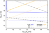 |
Fig. 3. Cooling timescales for protons, as a function of energy, for two galaxies with Ṁ∗ = 0.005 (solid lines) and 200 M⊙ yr−1 (dotted lines), in the base (0) scenarios. The blue and yellow lines indicate p-p scattering and ionisation, respectively. The black lines represent diffusion timescales (dot-dashed and dashed for K0 and B0 scenarios, respectively), whereas the grey double-dot-dashed line is the advection timescale. |
In Fig. 4 we show the escape and cooling times for electrons, at the same extreme SFRs plotted in Fig. 3, for the base scenarios K0 and B0. Diffusion can be neglected in both scenarios except for a small energy range around 1 GeV in scenario K0. Advection is the dominant energy loss mechanism for electrons at low electron energies (≲1 GeV), for low-SFR galaxies, whereas at higher energies electrons are cooled by synchrotron emission. As SFR increases, the time scales for Bremsstrahlung and ionisation (both  ) decrease, and these processes become dominant below ∼10 GeV. IC (with a time scale
  ) gets stronger and competes with synchrotron emission at higher energies. For Ṁ∗ ≳ 1 M⊙ yr−1 the system becomes a perfect electron calorimeter.
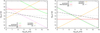 |
Fig. 4. Escape and cooling timescales for electrons, as a function of energy, for two galaxies with Ṁ∗ = 0.005 (left panel) and 200 M⊙ yr−1 (right panel), in the base (0) scenarios. The solid lines in different colours represent different cooling processes: ionisation (yellow), Bremsstrahlung (red), IC (green), and synchrotron (pink). The black lines indicate diffusion (dot-dashed and dashed for K0 and B0 scenarios, respectively), and the grey double-dot-dashed line indicates advection. |
4.2. Spectral energy distributions
The SED for the two extreme SFRs can be seen in Fig. 5 for base scenarios K0 and B0. To compare the emission of galaxies with different SFRs, we normalise the SED dividing the luminosity by the SFR. Within the Fermi energy range (the grey shaded region in Fig. 5), the SED comprises contributions IC, Bremsstrahlung, and p-p. Although IC emission grows with SFR faster than p-p, the latter dominates over the entire SFR range. This result agrees with those of previous authors (e.g. Lacki & Thompson 2013; Peretti et al. 2019).
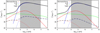 |
Fig. 5. Spectra energy distributions per unit SFR for galaxies in scenarios B0 (left panel) and K0 (right panel). The luminosity divided by the SFR, |
The prevalence of p-p radiation is due to two facts. First, the hadron-to-lepton ratio for CRs in SFGs is high (we adopted a = 50, see Sect. 3). Second, according to our model, most of the power of CR electrons is not radiated but rather lost by ionisation. The maximum energy these electrons radiate is ∼26% of the total energy injected into them. The case of protons is different, since ionisation losses are negligible and only escape processes compete with radiation losses.
At high SFRs, the γ-ray spectrum is similar in both base scenarios (K0 and B0). The spectral index for K0 is α* ∼ −2.3, a little bit steeper than that for B0 (α* ∼ −2.2), because of the strong diffusion. These values agree with the observed spectral indices of SBGs (Ajello et al. 2020). As SFR decreases, proton leakage begins to gain relevance. In the scenario B0, particles escape by advection, keeping α* unchanged. In K0, protons escape by diffusion, steepening α* to ∼ − 2.4 at Ṁ∗ = 0.005 M⊙ yr−1. Figure 6 shows that the agreement between modelled and observed SEDs is fairly good.
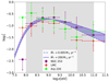 |
Fig. 6. Observed normalised SEDs ( |

4.3. Model Lγ–SFR relation
In Fig. 7 (left panel) we show the model Lγ–SFR relation for scenarios with different values of R, the radius of the region where CRs cool. The quantity Lγ is computed by integrating the SEDs between 0.1 and 100 GeV, for the 20 model galaxies of each scenario. We compare the model relations with that derived from the BF sample (see Sect. 2).
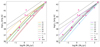 |
Fig. 7. Model Lγ–SFR relation for our scenarios 0, 1, and 2 (R = 1, 0.1, 5 kpc, left panel), and 0, 3, and 4 (vw = 400, 40, 4000 km s−1, right panel). Scenarios with both Kolmogorov (solid lines) and Bohm (dashed lines) diffusion prescriptions are shown. The black dotted line delineates the genuine calorimetric limit given by Eq. (18) (see text), whereas the grey dot-dashed line represents all the luminosity available in relativistic protons for each SFR. The grey shaded band indicates the 1σ confidence region of the fit to the BF sample (see Sect. 2). |
We showed in Sect. 4.2 that in the Fermi energy range, the main contribution to Lγ in our model is due to p-p radiation. Therefore, the Lγ–SFR relation is regulated by the leakage of protons from the CR cooling region. The absolute maximum power available for γ-ray radiation is the CR luminosity of Eq. (6), which scales linearly with the SFR (grey dot-dashed lines in Fig. 7). However, this limit is unreachable, as only ∼33% of the proton energy can be transformed into γ-ray photons (Kelner et al. 2006) and, according to the SEDs produced by our models, only ∼76% of the γ-ray luminosity is emitted in the Fermi band. This gives a more genuine limit for the γ-ray luminosity of the model galaxies (black dotted lines in Fig. 7),
![$$ \begin{aligned} L_{\gamma ,\mathrm{max}} [\mathrm{erg\,s}^{-1}] = 8.38 \times 10^{39} \dot{M}_* [{M}_\odot \,\mathrm{yr}^{-1}]. \end{aligned} $$](/articles/aa/full_html/2020/09/aa38428-20/aa38428-20-eq30.gif)
The departure of the emission from this limit, ρ = Lγ/Lγ, max, is therefore a measure of the ratio of the radiated to available power, or the calorimetric ratio. From the results of Sect. 2, for the observed data  . It is noteworthy that all galaxies, except NGC 3424 and NGC 4945 (which are outliers in other senses, see Sect. 2), lie below Lγ, max to within observational uncertainties. This result is not expected a priori, since the computation of Lγ, max includes model-dependent factors. Therefore, it suggests that the model effectively captures the relevant physics of the problem.
Figure 7 (left panel) shows that for all values of R, model galaxies approach the genuine Fermi limit at high SFRs (ρ → 1), whereas at lower SFRs they depart from this limit. The separation increases in a monotonic way as the SFR decreases. This is a density effect; high-SFR systems have higher ISM densities by construction, making p-p cooling more efficient and dominant over escape mechanisms. On the other hand, at low SFRs, the density is not high enough to prevent the escape of an important fraction of the proton population, leaving less energy to be transformed into γ-rays (ρ → 0). This result is consistent with previous works (Lacki & Thompson 2013; Wang & Fields 2018; Peretti et al. 2019).
At high SFRs (log Ṁ∗ [M⊙ yr−1] ≳ 0.5), the observed trend is well reproduced by our base scenario K0 (R = 1 kpc, Kolmogorov diffusion). The Bohm diffusion recipe (B0) shows a similar trend, but displaced from the locus of the observed galaxies. We recall that in B0 proton escape is driven by advection, at a slower rate. Therefore, B0 results in a higher calorimetric ratio than that of K0. Scenarios with larger radii (K2, B2, R = 5 kpc) underpredict the calorimetric ratio, because although larger systems have lower escape rates (τadv ∝ R, τdiff ∝ R2), they also have lower densities (at fixed SFR, τpp ∝ n−1 ∝ R2.42) that make p-p cooling much less efficient. These scenarios also show a steeper increase of ρ with SFR than that observed. On the other hand, the opposite is true for scenarios with small radii (K1, B1, R = 0.1 kpc). These are efficient calorimeters, and present ρ(Ṁ∗) trends shallower than that observed in our sample. Particularly, for Bohm diffusion (B1) we obtain ρ ≈ 1 in the whole high-SFR range, which means Lγ ∝ Ṁ∗. To summarise, at high SFRs our model is consistent with kiloparsec-sized CR cooling regions. Smaller regions are not ruled out, but require that diffusion proceeds in the Kolmogorov regime.
At low SFRs (log Ṁ∗ [M⊙ yr−1] ≲ −0,5), all scenarios fail to reproduce the observed trend. In all cases the Lγ–SFR relation is steeper than that observed. This suggests that the model overestimates the relative strength of escape with respect to p-p losses, for any size of the system.
To assess the effects of variations in the galactic wind velocity, in Fig. 7 (right panel) we show the same relations of left panel, but for scenarios 3 and 4. As expected, higher wind velocities increase the escape, lowering and steepening the curves with respect to scenarios K0 and B0. On the contrary, lower velocities move the curves closer to the calorimetric limit and make them shallower. At high SFRs, our model is consistent with mild to high wind velocities of several hundreds of kilometres per second. Slower winds cannot be discarded, but require the presence of Kolmogorov diffusion. Once again, at low SFRs, all scenarios fail to reproduce the observed trend because the curves are steeper than the relation determined from observations.
Finally, variations in the model magnetic field (scenarios 5 and 6) change the diffusion rate in the Bohm case as well as synchrotron losses. We already proved both processes to produce negligible effects. The results of scenarios 5 and 6 (for both diffusion prescriptions) show that the Lγ–SFR relation is not affected by changing the magnetic field, therefore, we do not discuss the latter further.
It is noteworthy that all scenarios fail in the same way at low SFRs. The Lγ–SFR relation shows a remarkably constant power-law index m = 1.71 in this SFR range, for all scenarios. This is different from the value m = 1.35 ± 0.05 obtained from observations. We defer a thorough discussion of this result to Sect. 5, noting that only four galaxies lie in this SFR range, and that three of these (all but the SMC) seem to follow the model trend more closely.
5. Discussion and conclusions
In this work we have compiled from the literature a near-homogeneous sample of distances and observed fluxes in the FUV, Hα, and IR, for all SFGs detected in γ-rays by Fermi. We used these data to obtain a self-consistent set of SFRs, and γ-ray and IR luminosities, to probe possible biases present in the Lγ–SFR correlation found by previous authors (Ackermann et al. 2012; Ajello et al. 2020). Our work improves on that of Ajello et al. (2020) by including a CR emission model describing this correlation for their full data set. Previous works have used smaller data sets, although they developed more refined models (e.g. Pfrommer et al. 2017) or explored different aspects of the correlation, such as the radio emission of SFGs (e.g. Ackermann et al. 2012).
Using the constructed sample, we show that LIR consistently underestimates the SFR of γ-ray emitting galaxies for Ṁ⊙ ≲ 1 M⊙ yr−1. Although this is a known result for the general galaxy population (Kennicutt et al. 2008; Kennicutt & Evans 2012), we stress this result because it produces a bias in the Lγ–LIR correlation, usually not corrected for (but see Pfrommer et al. 2017; Zhang et al. 2019). We quantified this bias, finding that the power-law index of the Lγ–SFR relation is underestimated by 0.14 when LIR is used as an SFR tracer. According to our data, the most probable value for this index is 1.35 ± 0.05, although the present sample is small (15 galaxies, with some outliers) and errors are relatively large, mainly due to large distance uncertainties. In any case, a linear Lγ–SFR relation is discarded with high confidence.
As a by-product, we find that at intermediate SFRs 0.3 ≲ Ṁ∗ ≲ 3 M⊙ yr−1, the dispersion of the Lγ–SFR relation is tens of times higher than outside this range. The MW is the only intermediate-SFR galaxy standing below the best-fit correlation, whereas the other four galaxies (NGC 2403, NGC 3424, NGC 4945, and Circinus galaxy) lie well above this correlation. The MW and NGC 4945 have almost the same SFR, but their luminosities differ by 1.37 dex. An objection might be raised that the MW γ-ray luminosity is modelled instead of measured, but the MW model fits γ-ray, radio, and CR data, therefore it is reliable and the discrepancy cannot be attributed to this fact. On the other hand, all four objects lying above the fit have suspected or confirmed AGNs (Yang et al. 2009; Gavazzi et al. 2011; Yaqoob 2012; Peng et al. 2019b), whereas the MW has a starving black hole in its centre (Schödel et al. 2002). Therefore, we suggest that the large dispersion of the Lγ–SFR relation in the intermediate SFR range is due to an AGN component in Lγ, whose strength varies from galaxy to galaxy. We argue that this component is not observable in other SFR ranges because low-SFR spirals have no AGN, whereas in ULIRGs the AGN emission may be highly absorbed by the dense ISM. At densities of 3 × 104 cm−3, typical of the innermost regions of SBG nuclei, pair production in the nuclear electric field of H I would provide the required absorption mechanism for gigaelectronvolt photons (Tanabashi et al. 2018). The confirmation of this claim, namely that AGNs contribute to the γ-ray luminosity of intermediate-SFR galaxies, would require the development of a method to separate the stellar-population component from that of the AGN in γ-ray observations. Such a method would certainly improve the observed Lγ–SFR relation.
A different possibility would be that Lγ comprises in some galaxies contributions from other sources, such as halo super-bubbles created by strong winds like those modelled by Romero et al. (2018). Alternative explanations would be that the power-law nature of the Lγ–SFR relation breaks at intermediate SFRs, producing a bump, or that normal spirals and SBGs follow different relations, which coexist in the mid-SFR range. In this case, extra observables would be needed to separate galaxies in both regimes. An exploration of this hypothesis will be addressed in a future work.
To explore the physics behind the observed Lγ–SFR relation, we developed a simple leaky-box model to compute the CR populations in SFGs, and their high-energy emission. Our Fermi-band model SEDs agree with those observed (Ajello et al. 2020). The emission is dominated by p-p inelastic scattering, in agreement with previous works (Lacki & Thompson 2013; Peretti et al. 2019), the leptonic radiation being negligible. The genuine calorimetric limit resulting from our model (which takes into account that only a fraction of the proton energy can be radiated) closely matches the emission of the highest-SFR systems, indicating that the model includes the relevant physics of γ-ray emission in SFGs.
Our model describes fairly well the Lγ–SFR relation at high SFRs, provided that CR cooling occurs in kiloparsec-sized regions, and galactic winds blow at velocities of several hundreds of kilometres per second. This is in line with the findings of de los Reyes & Kennicutt (2019) that star formation regions in galaxies are smaller than galactic discs by a factor of almost two. In this regard, our model disagrees with those previously used to compute the γ-ray emission of SBGs, which assume that the emission arises from spherical regions of ∼0.2 kpc in radius (e.g. Peretti et al. 2019). The discrepancy may be due to the different geometries used, as different sizes are required to reach a similar proton density, which is the variable that controls p-p emission. Our model also disagrees with the simulations of Pfrommer et al. (2017), who show γ-ray emission extending to ∼10 kpc-sized regions in galactic discs in their Fig. 1. The solution of these discrepancies requires spatially resolved γ-ray observations, not available at present for galaxies beyond the Local Group.
At low SFRs, our model predicts a steeper trend than observed, implying that the increase of particle escape with SFR has been overestimated. The power-law index of our model relation as Ṁ∗ → 0 reaches a limit of 1.71. This is because for small densities (implied by the K-S law),  , from Eqs. (6), (13), and (17) (once again, the K-S law), and the fact that escape does not depend on SFR owing to the constancy of R and vw. It is noteworthy that assuming that advection dominates through neutral winds like those observed by Martin (2005) and Weiner et al. (2009), we would obtain
  , rendering
  , in excellent agreement the value of 1.35 ± 0.05 derived by us from observations. In our model, advection dominates in scenarios with Bohm diffusion or in fast-wind scenarios with any diffusion prescription. However, as explained in Sect. 3, our Kolmogorov recipe represents the fastest diffusion, which is a very extreme situation. A lower normalisation of the Kolmogorov diffusion coefficient, such as that used by Peretti et al. (2019) in their model A, would provide an advection-dominated regime in our scenarios with Kolmogorov diffusion as well. This is the most plausible explanation of the observed trend at low SFRs: the Lγ–SFR relation may be driven by the combination of CR luminosity, the K-S law, and an advection-dominated escape regime with an SFR-dependent wind velocity. This explanation would also alleviate the tension of our model with present limits for the MW wind velocity, restricted to some tens of kilometres per second (e.g. Strong et al. 2007). These SFR-dependent wind velocities can arise in different scenarios (e.g. Veilleux et al. 2005, and references therein), including CR-driven winds (e.g. Girichidis et al. 2016); these scenarios are a promising clue to explore in follow-up works.
To summarise, we have provided strong evidence for the existence of a bias in previous determinations of the Lγ–SFR relation of SFGs owing to the use of IR luminosity as an SFR tracer. A quantitative estimation of the actual power-law index of this relation is 1.35 ± 0.05. Physically motivated, population-orientated models of γ-ray emission show that the unbiased relation can be explained at high SFRs by assuming that the CR cooling region is kiloparsec-sized and is pervaded by mild to fast winds. Combined with previous results about the scaling of wind velocity with SFR, our work provides support to advection as the dominant CR escape mechanism in low-SFR galaxies. The question of whether the emission of normal SFGs and SBGs is based on the same relevant physics, or if two different relations apply, is still open. A step forward in the comprehension of γ-ray emission by the stellar populations of SFGs requires further observations to enlarge the present sample and reduce measurement errors along with a reliable technique to disentangle the stellar contribution from that of the AGN, if present. On the theoretical side, population-orientated models may provide further insight into the conditions prevailing in SFGs, as far as the accuracy of present SFR scaling relations is improved, and new SFR scaling relations are unveiled.
Acknowledgments
PK and LJP acknowledge support from Argentine CONICET (PIP-2014-00265). Part of this work was supported by the German Deutsche Forschungsgemeinschaft, DFG project number Ts 17/2–1. JFAC acknowledges support from UNRN funds (project 40-C-691). JFAC is a staff researcher of the CONICET. GER was supported by the Argentine agency CONICET (PIP 2014-00338) and the Spanish Ministerio de Economía y Competitividad (MINECO/FEDER, UE) under grant AYA2016-76012-C3-1-P. This research has made use of the NASA/IPAC Extragalactic Database (NED), which is funded by the National Aeronautics and Space Administration and operated by the California Institute of Technology.
References
- Abdo, A. A., Ackermann, M., Ajello, M., et al. 2010a, ApJS, 188, 405 [NASA ADS] [CrossRef] [Google Scholar]
- Abdo, A. A., Ackermann, M., Ajello, M., et al. 2010b, ApJ, 709, L152 [Google Scholar]
- Abdollahi, S., Acero, F., Ackermann, M., et al. 2020, ApJS, 247, 33 [NASA ADS] [CrossRef] [Google Scholar]
- Acciari, V. A., Aliu, E., Arlen, T., et al. 2009, Nature, 462, 770 [NASA ADS] [CrossRef] [PubMed] [Google Scholar]
- Acero, F., Aharonian, F., Akhperjanian, A. G., et al. 2009, Science, 326, 1080 [NASA ADS] [CrossRef] [PubMed] [Google Scholar]
- Ackermann, M., Ajello, M., Allafort, A., et al. 2012, ApJ, 755, 164 [NASA ADS] [CrossRef] [Google Scholar]
- Ackermann, M., Albert, A., Atwood, W. B., et al. 2016, A&A, 586, A71 [NASA ADS] [CrossRef] [EDP Sciences] [Google Scholar]
- Adebahr, B., Krause, M., Klein, U., et al. 2013, A&A, 555, A23 [NASA ADS] [CrossRef] [EDP Sciences] [Google Scholar]
- Ajello, M., Mauro, M. D., Paliya, V. S., & Garrappa, S. 2020, ApJ, 894, 88 [CrossRef] [Google Scholar]
- Artale, M. C., Tissera, P. B., & Pellizza, L. J. 2015, MNRAS, 448, 3071 [NASA ADS] [CrossRef] [Google Scholar]
- Axford, W. I., Leer, E., & Skadron, G. 1977, Int. Cosm. Ray Conf., 11, 132 [Google Scholar]
- Bell, A. R. 1978, MNRAS, 182, 147 [NASA ADS] [CrossRef] [Google Scholar]
- Berezinsky, V. S. 1990, Int. Cosm. Ray Conf., 11, 115 [Google Scholar]
- Blandford, R. D., & Ostriker, J. P. 1978, ApJ, 221, L29 [Google Scholar]
- Blasi, P. 2010, MNRAS, 402, 2807 [NASA ADS] [CrossRef] [Google Scholar]
- Blom, J. J., Paglione, T. A. D., & Carramiñana, A. 1999, ApJ, 516, 744 [NASA ADS] [CrossRef] [Google Scholar]
- Blumenthal, G. R., & Gould, R. J. 1970, Rev. Mod. Phys., 42, 237 [NASA ADS] [CrossRef] [Google Scholar]
- Brauher, J. R., Dale, D. A., & Helou, G. 2008, ApJS, 178, 280 [NASA ADS] [CrossRef] [Google Scholar]
- Bustard, C., Zweibel, E. G., & Cotter, C. 2017, ApJ, 835, 72 [NASA ADS] [CrossRef] [Google Scholar]
- Chabrier, G. 2003, ApJ, 586, L133 [NASA ADS] [CrossRef] [Google Scholar]
- Chomiuk, L., & Povich, M. S. 2011, AJ, 142, 197 [NASA ADS] [CrossRef] [Google Scholar]
- Cortese, L., Boissier, S., Boselli, A., et al. 2012, A&A, 544, A101 [NASA ADS] [CrossRef] [EDP Sciences] [Google Scholar]
- Cowsik, R., Pal, Y., Tandon, S. N., & Verma, R. P. 1967, Phys. Rev., 158, 1238 [CrossRef] [Google Scholar]
- Crain, R. A., McCarthy, I. G., Frenk, C. S., Theuns, T., & Schaye, J. 2010, MNRAS, 407, 1403 [NASA ADS] [CrossRef] [Google Scholar]
- de Cea del Pozo, E., Torres, D. F., Rodriguez, A. Y., & Reimer, O. 2009, ArXiv e-prints [arXiv:0912.3497] [Google Scholar]
- de los Reyes, M. A. C., & Kennicutt, R. C., Jr. 2019, ApJ, 872, 16 [NASA ADS] [CrossRef] [Google Scholar]
- Domingo-Santamaría, E., & Torres, D. F. 2005, A&A, 444, 403 [NASA ADS] [CrossRef] [EDP Sciences] [Google Scholar]
- Draine, B. T. 2011, Physics of the Interstellar and Intergalactic Medium (Princeton: Princeton University Press) [Google Scholar]
- For, B. Q., Koribalski, B. S., & Jarrett, T. H. 2012, MNRAS, 425, 1934 [NASA ADS] [CrossRef] [Google Scholar]
- Gabici, S., Evoli, C., Gaggero, D., et al. 2019, Int. J. Mod. Phys. D, 28, 1930022 [Google Scholar]
- Gaisser, T. K., Engel, R., & Resconi, E. 2016, Cosmic Rays and Particle Physics (Cambridge: Cambridge University Press) [Google Scholar]
- Gavazzi, G., Savorgnan, G., & Fumagalli, M. 2011, A&A, 534, A31 [NASA ADS] [CrossRef] [EDP Sciences] [Google Scholar]
- Gil de Paz, A., Boissier, S., Madore, B. F., et al. 2007, ApJS, 173, 185 [Google Scholar]
- Ginzburg, V. L., & Syrovatskii, S. I. 1964, The Origin of Cosmic Rays (New York: Macmillan) [Google Scholar]
- Girichidis, P., Naab, T., Walch, S., et al. 2016, ApJ, 816, L19 [NASA ADS] [CrossRef] [Google Scholar]
- Griffin, R. D., Dai, X., & Thompson, T. A. 2016, ApJ, 823, L17 [NASA ADS] [CrossRef] [Google Scholar]
- Harris, J., & Zaritsky, D. 2004, AJ, 127, 1531 [NASA ADS] [CrossRef] [Google Scholar]
- Harris, J., & Zaritsky, D. 2009, AJ, 138, 1243 [NASA ADS] [CrossRef] [Google Scholar]
- Hinshaw, G., Larson, D., Komatsu, E., et al. 2013, ApJS, 208, 19 [NASA ADS] [CrossRef] [Google Scholar]
- Israel, F. P. 1997, A&A, 328, 471 [NASA ADS] [Google Scholar]
- Jokipii, J. R., & Morfill, G. E. 1985, ApJ, 290, L1 [NASA ADS] [CrossRef] [Google Scholar]
- Kelner, S. R., Aharonian, F. A., & Bugayov, V. V. 2006, Phys. Rev. D, 74, 034018 [NASA ADS] [CrossRef] [Google Scholar]
- Kennicutt, R. C., Jr. 1998, ApJ, 498, 541 [NASA ADS] [CrossRef] [Google Scholar]
- Kennicutt, R. C., Jr., & Evans, N. J. 2012, ARA&A, 50, 531 [NASA ADS] [CrossRef] [Google Scholar]
- Kennicutt, R. C., Jr., Lee, J. C., Funes, J. G., et al. 2008, ApJS, 178, 247 [NASA ADS] [CrossRef] [Google Scholar]
- Khangulyan, D., Aharonian, F. A., & Kelner, S. R. 2014, ApJ, 783, 100 [NASA ADS] [CrossRef] [Google Scholar]
- Lacki, B. C., & Thompson, T. A. 2013, ApJ, 762, 29 [CrossRef] [Google Scholar]
- Lanz, L., Zezas, A., Brassington, N., et al. 2013, ApJ, 768, 90 [NASA ADS] [CrossRef] [Google Scholar]
- Lenain, J. P., Ricci, C., Turler, M., Dorner, D., & Walter, R. 2010, Proceedings of the 25th Texas Symposium on Relativistic Astrophysics. December 6–10, 2010. Heidelberg, Germany [Google Scholar]
- Martin, C. L. 2005, ApJ, 621, 227 [Google Scholar]
- Merten, L., Becker Tjus, J., Eichmann, B., & Dettmar, R.-J. 2017, Astropart. Phys., 90, 75 [NASA ADS] [CrossRef] [Google Scholar]
- Nasonova, O. G., de Freitas Pacheco, J. A., & Karachentsev, I. D. 2011, A&A, 532, A104 [NASA ADS] [CrossRef] [EDP Sciences] [Google Scholar]
- Padilla, N. D., & Strauss, M. A. 2008, MNRAS, 388, 1321 [NASA ADS] [Google Scholar]
- Peng, F.-K., Wang, X.-Y., Liu, R.-Y., Tang, Q.-W., & Wang, J.-F. 2016, ApJ, 821, L20 [NASA ADS] [CrossRef] [Google Scholar]
- Peng, F.-K., Xi, S.-Q., Wang, X.-Y., Zhi, Q.-J., & Li, D. 2019a, A&A, 621, A70 [CrossRef] [EDP Sciences] [Google Scholar]
- Peng, F.-K., Zhang, H.-M., Wang, X.-Y., Wang, J.-F., & Zhi, Q.-J. 2019b, ApJ, 884, 91 [CrossRef] [Google Scholar]
- Peretti, E., Blasi, P., Aharonian, F., & Morlino, G. 2019, MNRAS, 487, 168 [CrossRef] [Google Scholar]
- Peretti, E., Blasi, P., Aharonian, F., Morlino, G., & Cristofari, P. 2020, MNRAS, 493, 5880 [CrossRef] [Google Scholar]
- Persic, M., & Rephaeli, Y. 2012, J. Phys. Conf. Ser., 355, 012038 [NASA ADS] [CrossRef] [Google Scholar]
- Persic, M., Rephaeli, Y., & Arieli, Y. 2008, A&A, 486, 143 [NASA ADS] [CrossRef] [EDP Sciences] [Google Scholar]
- Pfrommer, C., Pakmor, R., Simpson, C. M., & Springel, V. 2017, ApJ, 847, L13 [NASA ADS] [CrossRef] [Google Scholar]
- Rephaeli, Y., Arieli, Y., & Persic, M. 2010, MNRAS, 401, 473 [NASA ADS] [CrossRef] [Google Scholar]
- Rojas-Bravo, C., & Araya, M. 2016, MNRAS, 463, 1068 [NASA ADS] [CrossRef] [Google Scholar]
- Romero, G. E., & Torres, D. F. 2003, ApJ, 586, L33 [NASA ADS] [CrossRef] [Google Scholar]
- Romero, G. E., Müller, A. L., & Roth, M. 2018, A&A, 616, A57 [CrossRef] [EDP Sciences] [Google Scholar]
- Salpeter, E. E. 1955, ApJ, 121, 161 [Google Scholar]
- Sanders, D. B., & Mirabel, I. F. 1996, ARA&A, 34, 749 [NASA ADS] [CrossRef] [Google Scholar]
- Sanders, D. B., Mazzarella, J. M., Kim, D. C., Surace, J. A., & Soifer, B. T. 2003, AJ, 126, 1607 [Google Scholar]
- Schlickeiser, R. 2002, Cosmic Ray Astrophysics (Berlin: Springer) [CrossRef] [Google Scholar]
- Schödel, R., Ott, T., Genzel, R., et al. 2002, Nature, 419, 694 [NASA ADS] [CrossRef] [PubMed] [Google Scholar]
- Strickland, D. K., & Heckman, T. M. 2009, ApJ, 697, 2030 [NASA ADS] [CrossRef] [Google Scholar]
- Strickland, D. K., Heckman, T. M., Colbert, E. J. M., Hoopes, C. G., & Weaver, K. A. 2004, ApJS, 151, 193 [NASA ADS] [CrossRef] [Google Scholar]
- Strong, A. W., Moskalenko, I. V., & Ptuskin, V. S. 2007, Ann. Rev. Nucl. Part. Sci., 57, 285 [NASA ADS] [CrossRef] [Google Scholar]
- Strong, A. W., Porter, T. A., Digel, S. W., et al. 2010, ApJ, 722, L58 [NASA ADS] [CrossRef] [Google Scholar]
- Sudoh, T., Totani, T., & Kawanaka, N. 2018, PASJ, 70, 49 [CrossRef] [Google Scholar]
- Tanabashi, M., Hagiwara, K., Hikasa, K., et al. 2018, Phys. Rev. D, 98, 030001 [NASA ADS] [CrossRef] [Google Scholar]
- Tang, Q.-W., Wang, X.-Y., & Tam, P.-H. T. 2014, ApJ, 794, 26 [NASA ADS] [CrossRef] [Google Scholar]
- Tully, R. B., & Fisher, J. R. 1988, Catalog of Nearby Galaxies (Cambridge: Cambridge University Press) [Google Scholar]
- Tully, R. B., Rizzi, L., Shaya, E. J., et al. 2009, AJ, 138, 323 [NASA ADS] [CrossRef] [Google Scholar]
- Tully, R. B., Courtois, H. M., & Sorce, J. G. 2016, AJ, 152, 50 [NASA ADS] [CrossRef] [Google Scholar]
- Veilleux, S., Cecil, G., & Bland-Hawthorn, J. 2005, ARA&A, 43, 769 [Google Scholar]
- Völk, H. J., Aharonian, F. A., & Breitschwerdt, D. 1996, Space Sci. Rev., 75, 279 [Google Scholar]
- Wang, X., & Fields, B. D. 2018, MNRAS, 474, 4073 [NASA ADS] [CrossRef] [Google Scholar]
- Weiner, B. J., Coil, A. L., Prochaska, J. X., et al. 2009, ApJ, 692, 187 [NASA ADS] [CrossRef] [Google Scholar]
- Wilke, K., Klaas, U., Lemke, D., et al. 2004, A&A, 414, 69 [NASA ADS] [CrossRef] [EDP Sciences] [Google Scholar]
- Yang, Y., Wilson, A. S., Matt, G., Terashima, Y., & Greenhill, L. J. 2009, ApJ, 691, 131 [NASA ADS] [CrossRef] [Google Scholar]
- Yaqoob, T. 2012, MNRAS, 423, 3360 [NASA ADS] [CrossRef] [Google Scholar]
- Yoast-Hull, T. M., Gallagher, J. S., III, Zweibel, E. G., & Everett, J. E. 2014, ApJ, 780, 137 [NASA ADS] [CrossRef] [Google Scholar]
- Zhang, Y., Peng, F.-K., & Wang, X.-Y. 2019, ApJ, 874, 173 [CrossRef] [Google Scholar]
- Zirakashvili, V. N., & Aharonian, F. 2007, A&A, 465, 695 [NASA ADS] [CrossRef] [EDP Sciences] [Google Scholar]
All Tables
Distances, SFRs, IR, and γ-ray fluxes and luminosities for all γ-ray emitting SFGs known.
Values of the free parameters of our model (magnetic field of the galaxy, wind velocity, and radius of the CR cooling region) for the different scenarios considered.
All Figures
|
Fig. 1. Upper panel: SFR as a function of IR luminosity for our sample galaxies. The red dot-dashed and grey dashed lines represent the Ṁ∗(LIR) scaling relation presented in Eq. (3) for ϵ = 1 and 0.79, respectively. Lower panel: residuals of the Ṁ∗(LIR) relation for ϵ = 0.79, weighted by their standard deviation, as a function of LIR. The horizontal dotted lines correspond to ±3 standard deviations. |
| In the text | |
|
Fig. 2. Upper left panel: γ-ray luminosity of as a function of total IR luminosity for our sample. The grey solid line represents the best fit to the data (excluding the MW and NGC 3424) and the grey shaded region shows its 68% confidence level. The trend is consistent with those found by previous works. Lower left panel: residuals of the fit, weighted by their standard deviation, as a function of the total IR luminosity. The horizontal dotted lines correspond to ±3 standard deviations. Upper right panel: γ-ray luminosity as a function of SFR. Three fits performed on different data sets are shown: the full data set (cyan solid line); a reduced data set, excluding the MW and NGC 3424( green dashed line); and the BF, excluding all galaxies in the range −0.5 < log Ṁ∗ < 0.5 (grey dot-dashed line, see text). The grey shaded region shows the 68% confidence level of the BF fit. The red dotted line represents the best fit to the Lγ–LIR relation presented in the left panel, translated into the SFR–Lγ plane by Eq. (3), with ϵ = 0.79. The latter agrees only marginally with the data or any of the other three fits. Lower right panel: residuals of the BF fit, weighted by their standard deviation, as a function of the SFR. Horizontal dotted lines correspond to ±3 standard deviations. |
| In the text | |
|
Fig. 3. Cooling timescales for protons, as a function of energy, for two galaxies with Ṁ∗ = 0.005 (solid lines) and 200 M⊙ yr−1 (dotted lines), in the base (0) scenarios. The blue and yellow lines indicate p-p scattering and ionisation, respectively. The black lines represent diffusion timescales (dot-dashed and dashed for K0 and B0 scenarios, respectively), whereas the grey double-dot-dashed line is the advection timescale. |
| In the text | |
|
Fig. 4. Escape and cooling timescales for electrons, as a function of energy, for two galaxies with Ṁ∗ = 0.005 (left panel) and 200 M⊙ yr−1 (right panel), in the base (0) scenarios. The solid lines in different colours represent different cooling processes: ionisation (yellow), Bremsstrahlung (red), IC (green), and synchrotron (pink). The black lines indicate diffusion (dot-dashed and dashed for K0 and B0 scenarios, respectively), and the grey double-dot-dashed line indicates advection. |
| In the text | |
|
Fig. 5. Spectra energy distributions per unit SFR for galaxies in scenarios B0 (left panel) and K0 (right panel). The luminosity divided by the SFR, |
| In the text | |
|
Fig. 6. Observed normalised SEDs ( |
| In the text | |
|
Fig. 7. Model Lγ–SFR relation for our scenarios 0, 1, and 2 (R = 1, 0.1, 5 kpc, left panel), and 0, 3, and 4 (vw = 400, 40, 4000 km s−1, right panel). Scenarios with both Kolmogorov (solid lines) and Bohm (dashed lines) diffusion prescriptions are shown. The black dotted line delineates the genuine calorimetric limit given by Eq. (18) (see text), whereas the grey dot-dashed line represents all the luminosity available in relativistic protons for each SFR. The grey shaded band indicates the 1σ confidence region of the fit to the BF sample (see Sect. 2). |
| In the text | |
Current usage metrics show cumulative count of Article Views (full-text article views including HTML views, PDF and ePub downloads, according to the available data) and Abstracts Views on Vision4Press platform.
Data correspond to usage on the plateform after 2015. The current usage metrics is available 48-96 hours after online publication and is updated daily on week days.
Initial download of the metrics may take a while.