| Issue |
A&A
Volume 641, September 2020
|
|
|---|---|---|
| Article Number | A83 | |
| Number of page(s) | 13 | |
| Section | Stellar atmospheres | |
| DOI | https://doi.org/10.1051/0004-6361/202038397 | |
| Published online | 11 September 2020 | |
Superflares on the late-type giant KIC 2852961
Scaling effect behind flaring at different energy levels
1
Konkoly Observatory, Research Centre for Astronomy and Earth Sciences,
Budapest,
Hungary
e-mail: This email address is being protected from spambots. You need JavaScript enabled to view it.
2
Department of Physics, and Kavli Institute for Astrophysics and Space Research, Massachusetts Institute of Technology,
Cambridge,
MA
02139, USA
3
ELTE Eötvös Loránd University, Institute of Physics,
Budapest, Hungary
4
Department of Astrophysical Sciences, Princeton University,
NJ
08544, USA
Received:
11
May
2020
Accepted:
2
July
2020
Abstract
Context. The most powerful superflares reaching 1039 erg bolometric energy are from giant stars. The mechanism behind flaring is thought to be the magnetic reconnection, which is closely related to magnetic activity (including starspots). However, it is poorly understood how the underlying magnetic dynamo works and how the flare activity is related to the stellar properties that eventually control the dynamo action.
Aims. We analyze the flaring activity of KIC 2852961, a late-type giant star, in order to understand how its flare statistics are related to those of other stars with flares and superflares, and to understand the role of the observed stellar properties in generating flares.
Methods. We searched for flares in the full Kepler dataset of KIC 2852961 using an automated technique together with visual inspection. We cross-matched the flare-like events detected by the two different approaches and set a final list of 59 verified flares during the observing term. We calculated flare energies for the sample and performed a statistical analysis.
Results. The stellar properties of KIC 2852961 are revised and a more consistent set of parameters are proposed. The cumulative flare energy distribution can be characterized by a broken power law; that is to say, on the log-log representation the distribution function is fitted by two linear functions with different slopes, depending on the energy range fitted. We find that the total flare energy integrated over a few rotation periods correlates with the average amplitude of the rotational modulation due to starspots.
Conclusions. Flares and superflares seem to be the result of the same physical mechanism at different energy levels, also implying that late-type stars in the main sequence and flaring giant stars have the same underlying physical process for emitting flares. There might be a scaling effect behind the generation of flares and superflares in the sense that the higher the magnetic activity, the higher the overall magnetic energy released by flares and/or superflares.
Key words: stars: activity / stars: flare / stars: late-type / stars: individual: KIC 2852961 / stars: individual: TIC 137220334 / stars: individual: 2MASS J19261136+3803107
Juan Carlos Torres Fellow.
© ESO 2020
1 Introduction
Studying the cosmic neighborhood of magnetically active stars, that is to say the impact of stellar magnetism on the circumstellar environment where planets may revolve, is currently a hot issue. Stellar flares can heavily affect their close vicinity, such as how solar flares affect the Earth. The most energetic solar flares recorded so far, for example the “Carrington Event" in 1859, reached the energy output of 1033 erg (Cliver & Dietrich 2013). On the other hand, stellar flares can release one to six orders of magnitude more energy (Maehara et al. 2012) compared to the most powerful X-class solar flares; such “superflare stars" are mostly solar-like stars from the main sequence, but they can also be evolved stars in some measure, being either single or a member of a binary system (see, e.g. Balona 2015; Katsova et al. 2018; Notsu et al. 2019, and their references).
The high magnetic energy outbursts by flares are believed to originate from magnetic reconnection; this presumes an underlying dynamo action, that is to say rotation (differential rotation) interfering with convective motions. However, through stellar evolution, slower rotation and increased size are expected to result in weaker magnetic fields and therefore lower levels of magnetic activity for evolved stars compared with their main sequence progenitors. Yet, the most powerful superflares are from giants (Balona 2015). Just recently, cross-matching superflare stars from the Kepler catalogue with the Gaia DR-2 stellar radius estimates has shown that more than 40% of stars previously believed to be solar-type flare stars were actually subgiants (Notsu et al. 2019). Magnetic activity is present and can indeed be strong along the red giant branch, which has been verified by direct imaging of starspots on the K-giant ζ Andromedae (Roettenbacher et al. 2016). However, it is not clear what kind of mechanism could generate sufficient energy to provide the most powerful superflares on giant stars. It is quite certain that in some cases binarity plays a key role: a close companion star or a close-in giant planet could mediate magnetic reconnection and so provoke superflares (Ferreira 1998; Rubenstein & Schaefer 2000). Katsova et al. (2018) propose a magnetic dynamo working with antisolar differential rotation to explain the production of the most powerful superflares on giant stars. This is supported by the finding that, to date, only giant stars have been reported to exhibit antisolar differential rotation (see Kővári et al. 2017a, and their references). But besides the non-uniform rotation profile, convective turbulence should also play a crucial role in driving stellar dynamos. Just recently, Lehtinen et al. (2020) demonstrated that a common dynamo scaling can be achieved for late-type main sequence and evolved, post-main-sequence stars only when both stellar rotation and convection are taken into account. This finding implies that magnetic dynamo action-related flares in solar-type stars and superflares, for instance, in late-type giants, can be linked by scaling as well. The paradigm that dynamo action is necessary to produce flares, however, is nuanced by the recent finding that A-type stars without convective bulk can also have superflares (Balona 2015). On the other hand, this finding is questioned by Pedersen et al. (2017), who conclude that most of the A-type flare star candidates in Balona (2015) are binary stars and flares probably originate from an unresolved companion star.
Observing flares in giant stars from the ground is quite a challenge, first of all, because of the luminous background of the stellar surface. The most energetic flares of 1038 erg in the optical range would raise the brightness level of a red giant by only a few hundredths of magnitude at the peak. Such a small change is on the order of the brightness variability due to short-term redistribution of starspots; that is to say that, generally, flares in spotted giant stars can oftentimes be indistinguishable from a small change in the rotational modulation in the event of low data sampling and/or low data quality. At the same time, signals of less luminous flares would easily blend into the noise. Therefore, high precision space photometry from Kepler or TESS can be very useful in studying the optical signs of stellar activity in detail, including starspots and (super)flares, but it can also reveal such phenomena that are difficult or impossible to observe from the ground (e.g. oscillations). Moreover, space instruments can provide continuous observations (e.g. Baliunas et al. 1984; Ayres et al. 2001; Sanz-Forcada et al. 2002; Mullan et al. 2006), which are inevitably required to examine the temporal behavior of complex (multiple) flare events or make up flare statistics for individual targets (see also Davenport 2016; Vida et al. 2017, 2019; Günther et al. 2020, etc.).
In our study, we analyze the flaring activity of a target from the Kepler Input Catalog under the entry-name KIC 2852961 (2MASS J19261136+3803107, TIC 137220334) using Kepler and TESS observations. The star was listed in the ASAS catalog of variable stars in the Kepler field of view (Pigulski et al. 2009) with a 35.58 d rotation period, derived using 83 and 100 data points obtained in V and I colors, respectively,between May 28, 2006, and January 16, 2008. Figure 1 shows archival photometry from the Hungarian-made Automated Telescope Network (HATNet, Bakos et al. 2004) with 4475 datapoints in IC color collected during the observing season in 2006 (205 days). The folded light curve underneath, assuming Pphot = 34.27 d period, supports the idea that the photometric period of ≈35 days is indeed due to rotation. Additionally, the shape of the slowly changing light curve is typical of spotted stars. From a slightly earlier period, in the 2003 HATNet dataset, we found a large flare with an amplitude of about 0.08 mag in the infrared (i.e. well above the noise limit of ≈0.01 mag) but, unfortunately, with sparse coverage of the decay phase; see Fig. 2. We note that observing such an event from the ground is simply a matter of blind luck.
According to the NASA Exoplanet Archive1, the low surface gravity of log g = 2.919, a surface temperatureof 4722 K, and a radius of 5.5 R⊙, together with the ≈35 d rotation period, are all consistent with the preconception that KIC 2852961 is a late G-early K giant. The Kepler time series of our target was examined first by an automated Fourier-decomposition in Debosscher et al. (2011), who found signatures of rotational modulation with other non-classified signs of variability; however, the presumed eclipsing binary nature was not confirmed. In turn, based on new high-resolution spectroscopic data, KIC 2852961 has recently been categorized as a single-lined spectroscopic binary (SB1), but further details have not been provided (Gaulme et al. 2020). Our star is included in Balona (2015, see Table 2 in that paper) as a rotational variable but with a spurious period, as the short-cadence Kepler data did not cover the entire rotation. In the short-cadence data, Balona et al. (2015) searched for quasi-periodic pulsations (QPPs) induced by flares and found that KIC 2852961 indeed showed distinct “bumps" in the flare decay branches, which might be flare loop oscillations and are unlikely to be a sign of induced global acoustic oscillation.
In this study we use all the available Kepler and TESS light curves of KIC 2852961 in order to search for stellar flares and study their occurrence rate, which is the only study of its kind for a flaring giant star to date. The paper is organized as follows. In Sect. 2 our new spectroscopic observations are presented and analyzed. In Sect. 3 we revise the stellar parameters of KIC 2852961. In Sect. 4 we give a summary of the Kepler and TESS observations, while in Sect. 5 the applied data processing methods are described. The results are presented in Sects. 6–8 and discussed in Sect. 9. Finally, a short summary with conclusions is given in Sect. 10.
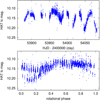 |
Fig. 1 HATNet photometry of KIC 2852961 collected in one observing season between May and December 2006. Top panel: observationsin I band vs. JD (2,400,000.0+), bottom panel: the folded light curve is plotted using Pphot = 34.27 d period. |
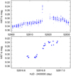 |
Fig. 2 A large flare of KIC 2852961 on June 26, 2003, observed by HATNet. The slowly changing base light curve shown between June 10 and July 10 covers nearly a whole rotation period. Apart from the flare, the volumes of the nightly changes indicate the overall scatter of the photometric measurements. |
Observing log of the spectroscopic data taken by the Hungarian 1-m RCC telescope.
2 Mid-resolution spectroscopic observations and data analysis
New mid-resolution spectroscopic observations were taken between April 4-8 and between May 1–3, 2020, by the 1-m RCC telescope of Konkoly Observatory, located at Piszkéstető Mountain Station, Hungary, equipped with an R = 21 000 échelle spectrograph. Altogether, 27 spectra were collected with two to five exposures per day, depending on weather conditions. Circadian exposures were combined to get eight combined spectra with total exposures between 1–3 h, yielding signal-to-noise ratios (S/Ns) larger than 40 for each. The spectra were reduced using standard IRAF2 échelle reduction tasks. Wavelength calibration was done using ThAr calibration lamps. The observational log is given in Table 1.
Radial velocity measurements were taken in respect to the radial velocity standard HD 159222 (Soubiran et al. 2018). The temporal variation of the radial velocity of KIC 2852961, with the estimated error bars, are given in the last two columns of Table 1 and plotted in Fig. 3. Despite the different weather conditions, which are reflected by the size of the error bars, the plot clearly shows that the radial velocity significantly decreased from ≈25 kms−1 in early April to ≈11 kms−1 in the beginning of May (i.e. over about 25 days). This change could indeed be a sign of orbital motion, in line with the SB1 nature suggested by Gaulme et al. (2020), but further observations are necessary to cover the full orbit.
Three of the best-quality combined spectra were used to estimate the rotational broadening of the spectral lines with spectral synthesis. We applied the spectral synthesis code SME (Spectroscopy Made Easy, Piskunov & Valenti 2017). Atomic line data were taken from the Vienna Atomic Line Database (Kupka et al. 1999) and MARCS atmospheric models (Gustafsson et al. 2008) were used. Keeping Teff, log g, and [Fe/H] as free parameters, the fits yielded Teff = 4810 ± 60 K, log g = 2.49 ± 0.10 [cgs], and [Fe/H] = −0.25 ± 0.10, with v sin i = 17.0 ± 1.2 kms−1. When Teff, log g, and [Fe/H] are kept constant as 4722 K, 2.43, and −0.08, respectively (see Table 2 in Sect. 3), the spectral fits yielded v sin i ≈18.0 kms−1 but with larger error bars. Henceforth, therefore, we accept v sin i = 17.5 kms−1 but draw attention to the fact that this result is preliminary due to the relatively low S/N of the spectra and the smearing effect from the medium resolution.
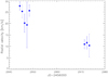 |
Fig. 3 Radial velocity measurements of KIC 2852961 taken by the 1-m RCC telescope at Piszkéstető Mountain Station, Konkoly Observatory, Hungary, between April 4 and May 3, 2020. |
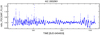 |
Fig. 4 Long-cadence Kepler data of KIC 2852961. Note the rotational variability that changes from one rotational cycle to the next,typical for stars with constantly renewing spotted surfaces. Several flare events are also present, including very large ones. |
3 Revised stellar parameters of KIC 2852961
The Gaia DR-2 parallax of 1.2845 ± 0.0259 mas (Gaia Collaboration 2018), taking into account a mean offset of –53.6 μas (cf. Fig. 1 in Zinn et al. 2019, and their references), yields a distance of 813 ± 17 pc for our target. According to the ASAS light curve (Pigulski et al. 2009), the brightest visual magnitude ever observed can be estimated as Vmax ≈ 10. m30. This, together with the above mentioned distance and an interstellar extinction of AV = 0. m264 from 2MASS (Skrutskie et al. 2006), gives us an absolute visual magnitude of MV = 0. m486 ± 0. m046. The effective temperature Teff =  K from the Kepler Input Catalog (Kepler Mission Team 2009), which is practically the same as the
  K from Gaia DR-2, is consistent with a bolometric correction of BC =
  (Flower 1996). This yields a bolometric magnitude of Mbol = 0. m032 ± 0. m090, convertible to
  . Taking this luminosity value, the Stefan-Boltzmann law would give us R = 13.1 ± 0.9 R⊙. This new radius is more than two times larger than the one listed in the NASA Exoplanet Archive; however, it is derived in a trustworthy way and is in better agreement with the radius of 10.64 R⊙ given in Gaia DR-2 (Gaia Collaboration 2018). The surface temperature and the derived luminosity are used to plot our target on the Hertzsprung–Russell (H-R) diagram in Fig. 5. Stellar evolution tracks are taken from Padova and Trieste Stellar Evolution Code (PARSEC, Bressan et al. 2012) for Z = 0.01 ([M/H] = −0.175). From Fig. 5, we estimate a stellar mass of 1.7 ± 0.2M⊙ for KIC 2852961 with an age of ≈1.7 Gyr (i.e. around the red giant bump). We note, however, that due to the uncertainty in metallicity, the true errors should be ≈50% larger compared with those estimated from Teff and luminosity only. The above mentioned mass and radius would yield a surface gravity of log g = 2.43 ± 0.14. While this is smaller by ≈20% compared to the value of 2.919 ± 0.145 given in the NASA Exoplanet Archive, it is more consistent with the revised astrophysical properties. Finally, taking v sin i of 17.5 kms−1, obtained from spectral synthesis (see Sect. 2), with the maximum equatorial velocity of 18.6 kms−1, calculated from the photometric period and the estimated radius, yields ≈70° inclination. The most important stellar parameters of KIC 2852961 are listed in Table 2.
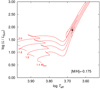 |
Fig. 5 Position of KIC 2852961 in the H-R diagram (dot). The stellar evolutionary tracks shown between 1.4 and 2.0 solar masses by 0.2 steps are taken from PARSEC (Bressan et al. 2012), adopting [M/H] = −0.175. From the location, the expected mass is around 1.7 M⊙. |
4 Observations from Kepler and TESS
The full Kepler dataset, available for KIC 2852961 in the NASA Exoplanet Archive, was collected between Barycentric Julian Dates (BJD) 2 454 953.5 and 2 456 424.0. A total of 19 Kepler light curves were observed, of which 18 were long-cadence time series from quarters Q0-Q17 with a time resolution (effective integration time) of 30 min, and one was a short-cadence light curve in Q4 with one minute sampling. The normalized long-cadence data are plotted in Fig. 4, indicating the rotational modulation due to spots together with strong flare activity. This time series was taken in order to search for the best-fit photometric period. For the computations, we used the Lomb-Scargle algorithm (Lomb 1976; Scargle 1982) in the Periodogram Tool of the NASA Exoplanet Archive. According to the resulting periodogram in Fig. 6, the strongest peak is located at Pphot ≈ 35.5 d; this is in pretty good agreement with other period determinations made using the ASAS and HATNet datasets (see Sect. 1). We notice that the bunch of peaks in the periodogram in Fig. 6, as well as the different main periods found for other datasets (ASAS, HATNet) observed at different times, might be an indication of surface differential rotation.
Additionally, we used TESS Sector 14 data taken between July 18 and August 15, 2019 (BJD 2454953.5–2 456 424.0). The 30-min cadence data were extracted using the eleanor pipeline3, an open-source tool to produce light curves for objects in the TESS full-frame images (FFI; Feinstein et al. 2019).
Revised astrophysical data of KIC 2852961.
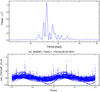 |
Fig. 6 Periodogram (top) and folded light curve (bottom) of KIC 2852961 using data shown in Fig. 4. The highest peak of the Lomb-Scargle periodogram indicates a rotation period of ≈35.5 d. Plots are created with the Periodogram Tool of the NASA Exoplanet Archive. |
5 Detecting flares in photometric data from space
We searched for flares using an automated technique accompanied by visual inspection. For this, we applied an updated version of the flare detection pipeline from Günther et al. (2020). We started from the detrended Kepler and TESS light curves and computed a Lomb-Scargle periodagram to identify (semi-)periodic modulation caused by stellar variability or rotation. The strongest periodic signal was removed using a spline with knots spaced at one-tenth of the detected period. At the same time, we searched for outliers by sigma clipping the data residuals, identifying and masking all outliers that were more than 3-σ away. We repeated this entire process two more times or until no new periods were found, collecting a list of all outliers. These outliers were considered to be flare-like events if they contained a series of at least three consecutive 3-σ outlier points.
These candidates were then re-examined manually to decide if they had a flare-like profile and could be declared a flare. To this end, the classical flare profile with a rapid rise followed by exponential decay branch helped in the verification. However, various doubtful cases were found at the low energy end, where quasi-oscillations, scatter, and instrumental glitches either hampered the detection or caused false positives. In the end, we confirmed 59 flare events in the Kepler time series (three of which were observed simultaneously in both short- and long-cadence data), while one single event was found in the much shorter TESS light curve.
6 Calculation of the flare energies
For each confirmed flare event, we calculated flare energies in the following way. We used I0 and I0+f to denote the intensity values (either bolometric or in a given bandpass) of the stellar surface at quiescent and flaring states, respectively.The flare energy relative to the star can be written as
 (1)
(1)
where t1 and t2 are the start and the end points of the given flare event. The quiescent stellar flux is estimated using black body approximation, where Planck’s law gives the spectral radiance:
 (2)
(2)
By integration over all solid angles of a hemisphere, the spectral exitance is πB(λ, T); therefore, the quiescent stellar luminosity through the Kepler filter would read
 (3)
(3)
where A⋆ is the stellar surface and  is the Kepler response function given between λ1 and λ2. At this point, the total integrated flare energy through the Kepler filter is obtained by multiplying the relative flare energy by the quiescent stellar luminosity:
 (4)
(4)
Taking R and Teff from Table 2, the quiescent stellar luminosity through the Kepler filter is L⋆Kep = 7.2 × 1034 erg s−1. (In comparison, the total bolometric luminosity from the Stefan-Boltzmann law is L⋆ = 2.85 × 1035 erg s−1.) The calculated Ef flare energies with the corresponding Tpeak peak times and Δt durations are listed in Table 3 together with the equivalent flare duration (teq) values. We note that this last value is identical to εf from Eq. (1), since it is basically the time interval in which the star would radiate as much energy as the given flare itself, that is
 (5)
(5)
In Quarter 4 of the Kepler season, where both long- and short-cadence data are available, the calculations are performed for three confirmed flare events detected simultaneously in both datasets (see Fig. 7). The derived corresponding flare energies (see rows 13–15 in Table 3) are quite close to one another, differing by only 1–6%. Therefore, we estimate that the uncertainty of our flare energy calculations is within ≈10%. On the other hand, flare energies can also be calculated by assuming black body continuum emission at around TBB = 8000−10 000 K (see, e.g. Kretzschmar 2011, and their references). Using the method in Shibayama et al. (2013), we recalculated some of our flare energies assuming that TBB = 9000 K, which yielded an ≈8% difference compared to the values in Table 3 (i.e. still within the 10% uncertainty). The best match was obtained when TBB ≈ 8300 K was used.
The above calculations were repeated for the TESS flare but using the TESS transmission function instead; for these results, see Table 4. We note that since the teq,TESS and Ef,TESS values in Table 4 are calculated using a different filter function, they therefore cannot be compared directly to the respective values of the Kepler flares in Table 3.
Among the flare events listed in Tables 3 and 4, the shortest ones last approximately five hours, while the longest one reached a length of two days, which is extremely long. The respective integrated energy values range between 1035 and 1038 ergs (i.e. they span over three orders of magnitude). In our case, 1035 erg multiplied by a factor of two or three should be regarded as the detection limit due to data noise and other reasons (e.g. quasi-oscillations, which slightly vary the overall brightness on a timescale of a few hours). On the high end of the energy range, some of the events show quite unusual structures. Such an event can be the result of multiple (regular or irregular) flare eruptions emerging at the same time, either in physical connection or independently by coincidence. However, other peculiarities should also be considered, such as the quasi-periodic pulsations (QPPs) in the decay phaseof a flare (Balona et al. 2015; Pugh et al. 2016; Broomhall et al. 2019). The flares observed in short cadence (see our Fig. 7) were reported to show QPPs in Pugh et al. (2016) and Balona et al. (2015).
Figure 8 shows two more examples from the list of flares in Table 3: one with a complex structure and another with a regular shape. The decay phase of the complex flare very likely shows indications of QPPs (cf. Pugh et al. 2016), even in long-cadence sampling. We note that complex events (marked with * symbols in Table 3) similar to the plotted one might also be the superimposition of a couple of simultaneous flares. Nevertheless, such a complex flare is regarded as one single event in our analysis, because in most cases it is nearly impossible to differentiate a real complex event from a series of individual flares overlapping each other in time. On the other hand, it is very likely that such simultaneous flare events are physically connected by sharing the same active region and may be triggering each other as well (Lippiello et al. 2008), that is to say, releasing magnetic energy from the same resource; therefore, it is reasonable to treat them as one event. As a third example, in Fig. 9 we show the only flare detected in the TESS light curve (see Table 4); it has a regular shape and lasted almost 40 h. The emitted energy of ≈ 5× 1037 erg in the TESSbandpass (visible-near infrared spectrum) classifies it as another fairly powerful superflare of KIC 2852961 (cf. Table 3).
 |
Fig. 7 Three flares observed on KIC 2852961 with short- and long-cadence in Kepler Q4. Short-cadence data are drawn with a thick blue line, while long-cadence data are overplotted with a thin red line. |
7 The cumulative flare frequency distribution
In order to investigate the dependence of flare occurrence on flare energy, we followed the method introduced by Gershberg (1972), who found that cumulative flare frequency distribution (FFD) for flare stars tended to follow a power law (see also Lacy et al. 1976). Accordingly, the ΔN(E) number of flares in the energy range E + ΔE per unit time (days) can be written as
 (6)
(6)
Rewriting this in a differential form and integrating between E and Emax (i.e. the cutoff energy), we get that the ν(E) cumulative number of flares with energy values larger than or equal to E is
 (7)
(7)
where c1 is a constant number. In logarithmic form this converts to
 (8)
(8)
a linear function between log ν and log E, where c2 and β = − α + 1 are constant numbers of the linear function, that is the intercept and the slope 1 − α, respectively.
It has been ascertained that the low energy turnover of the FFD is most probably the result of the detection threshold (cf. e.g. Hawley et al. 2014), that is to say the low S/N of small flares. Therefore, we ran flareinjection-recovery tests using the code allesfitter (Günther & Daylan 2019, 2020) to map out the detection bias in the low energy regime. First, we set a suitable grid of artificial flares over the full widths at half maximum (FWHM) and amplitudes of the flares, since these two properties feature the relative flare energy. The FWHM-amplitude grid was chosen to cover the relative flare energy range between teq = 0.0864–86.4 s, convertible to log Ef = 33.78–36.78 [erg] total logarithmic flare energy (see Eq. (6)). To make up the model flare light curves, allesfitter adopts the empirical flare template described in Davenport et al. (2014).
The artificial flares were injected into the original Kepler light curve, and then the flare detection algorithm (described in Sect. 5) was applied to recover them, thus statistically characterizing the recovery rate. The resulting injection-recovery plot is shown in Fig. 10, where blue gradient is used to visualize the recoveryrate as the function of FWHM and amplitude. From the test, we estimate a detection limit teq between 5–10 s, in agreement with the results in Table 3. Towards higher FWHM values and amplitudes (i.e. higher energies), the recovery rate increases up to the upper-right corner of the grid, where the recovery rate virtually reaches ≈100%. We derived correction factors (multiplicative inverses) from the recovery rates to estimate the real flare numbers at the low energy range. These estimations are used to plot the detection bias-corrected cumulative flare-frequency diagram.
The log–log representation of the FFD diagram is shown in Fig. 11. At low energy, the deviation from linear is nicely reduced compared to the gray dots, which indicate the original (uncorrected) frequencies. But more markedly, having a breakpoint at around E ≥ 5 × 1037 erg, the distribution deviates from linear, exhibiting a slight slope in the low energy region and a much steeper part at the high energy end. Fitting the lower energy range (see the green line in Fig. 11) yields α = 1.29 ± 0.02. (We note that a fit to the uncorrected distribution over the same energy range would yield α = 1.21 ± 0.02.) Applying another fit to the high energy range above the breakpoint at E ≥ 5 × 1037 erg gives α = 2.84 ± 0.06 (see the orange line in Fig. 11). This is significantly higher than the fit to the low energy part and higher than that usually derived for flaring dwarf stars (e.g. Howard et al. 2018; Paudel et al. 2018; Ilin et al. 2019; Yang & Liu 2019, etc.). For further discussion on the broken flare energy distribution diagram, see Sect. 9.2.
Peak times (BJD–2 454 833), flare durations, equivalent durations, and flare energies in the Kepler bandpass.
Peak time, duration, equivalent duration, and integrated flare energy in the TESS bandpass for the only flare detected in the TESS Sector 14 data.
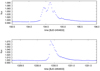 |
Fig. 8 Two examples for flare detections on KIC 2852961 by Kepler. Top panel: (very likely multiple) flare event of Ef = 2.273 1038 erg energy (Tpeak = 194.634 d in Table 3) with a complex, irregular shape. The superflare of Ef = 1.017 1038 erg shown in the bottom panel (Tpeak = 1330.395 d in Table 3) has a regular light curve. |
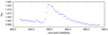 |
Fig. 9 Only flare event on KIC 2852961 found in our TESS Sector 14 data, showing a fairly regular shape; cf. Table 4. |
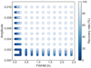 |
Fig. 10 Result of the injection-recovery test. Each circle on the plot represents a given model flare characterized by its FWHM and amplitude. The recovery rate of the model flares is represented by a blue gradient bar (the darker the shade, the lower the recovery rate). The energy range in total logarithmic flare energy extends from log E = 33.78 [erg] up to 36.78 [erg], where the recovery rate virtually reaches 100%. |
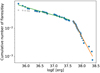 |
Fig. 11 Detection bias-corrected cumulative flare-frequency diagram for KIC 2852961. The original detection-biased datapoints are plotted in gray; above them are the corrected points in blue. The fit to the lower energy range below the breakpoint (green line) yields α = 1.29 ± 0.02 parameter, while the fit for the high energy range above the breakpoint (orange line) gives α = 2.84 ± 0.06. |
8 Correlation between spot modulation and flares
The light curve of KIC 2852961 in Fig. 4 shows significant change in the amplitude variation and the temporal distribution of flare occurrences throughout the whole mission. It is clear that: in the first third of the mission, KIC 2852961 performed large amplitude rotational modulation with a lot of energetic flares; in the middle of the term the amplitude got smaller and the flares got less powerful and occurred less frequently; at the end of the term, the amplitude increased again together with the average flare energies, although the flare frequency did not change much during the second half of the observing term. To quantify this observation, in Fig. 12 we plot the simple moving average of the overall amplitude change of the light curve cleaned from flares (top panel) together with the total flare energy within the same boxcar, which was set to be 3Prot (bottom panel). In the lower edge of the bottom panel, we mark the individual flare events with red ticks. The plot indicates that there is indeed a connection between the rotation amplitude (as an indicator of magnetic activity) and the overall magnetic energy released by flares. The second half of the observing term, starting with small amplitudes at BJD ≈ 700 (+2 454 833) with a few smaller flares, is especially interesting. After a few rotation periods, at around BJD ≈ 900, the amplitude starts to increase significantly, similar to the flare energies. This pattern is even more apparent from BJD ≈ 1300, where the amplitude of the rotational modulation increases more rapidly, which coincides with the overall flare energy increase (without the increase of the average flare count). This result suggests a general scaling effect behind the production of flares, in the sense that there are more and/or more energetic flares when there are more and/or larger active regions on the stellar surface, and that the flare activity is lower when there are fewer and/or smaller active regions. In Sect. 9.5 we elaborate a little more on this topic, while in Appendix A we demonstrate the reliability of the observed rotational amplitudes shown in Fig. 4.
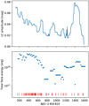 |
Fig. 12 Top: moving average of the amplitude of rotational modulation in the Kepler light curve of KIC 2852961 shown in Fig. 4. Bottom: total flare energy within the boxcar of 3Prot used for the moving average. The red tick marks below indicate the peak times of the flare events. See the text for details. |
9 Discussions
9.1 On the stellar evolution, rotation, and differential rotation
The revised stellar parameters of KIC 2852961 listed in Table 2 are in agreement with the new Gaia DR-2 observations and are more consistent with one another. The mass of about 1.7 M⊙ is considerably higher than the formerly suggested mass of ≈0.9 M⊙ (NASA Exoplanet Archive). The higher mass we find is also suggestive of a faster evolution or a younger age of ≈1.7 Gyr (which is tightly interrelated with mass). Taking the relation tMS ∝ M−2.5 between the main sequence period and mass with 0.9 M⊙ instead of 1.7 M⊙, and supposing no significant mass loss at the red giant branch (cf. e.g. McDonald & Zijlstra 2015), would mean a much slower evolution on the main sequence of tMS ≈13 Gyr; this would be unreasonably long. Using the mass-radius relation (see e.g. Mihalas & Binney 1981; Demircan & Kahraman 1991), one can estimate RMS ≈ 2.0 R⊙ for the main sequence, that is to say, a typical A5-F0 type progenitor (cf. Boyajian et al. 2012, 2013). Assuming that our SB1 target (cf. Gaulme et al. 2020) has a distant and/or too-low mass companion that has insignificantinfluence, and the angular momentum is conserved over the red giant branch, applying the relation Prot ∝ R2 will give Prot,MS of ≈1 d period at the end of the main sequence. This rotation rate is high but not unusual for an effectively single A5-F0 star just leaving the main sequence, since the lack of a deep convective envelope in stars with >1.3 M⊙ mass does not enable it to generate enough strong magnetic fields to maintain effective magnetic braking over the main sequence (van Saders & Pinsonneault 2013). Still, other mechanisms could also be considered to spin up the surface of an evolved star on the red giant branch. A certain fraction of red giants have undergone such spin-up phases (e.g. Carlberg et al. 2011; Ceillier et al. 2017), which may involve mixing processes (Simon & Drake e.g. 1989, but see also Kriskovics et al. 2014; Kővári et al. 2017b), planet engulfment (Siess & Livio 1999; Kővári et al. 2016), binary mergers (Webbink 1976; Strassmeier et al. 1998), or other, lesser known mechanisms. However, the lack of systematic radial velocity measurements does not enable us to know whether KIC 2852961 is a member of a wide binary system or a member of a close binary system. In the latter case, the stellar rotation is probably synchronized to the orbital motion, which would evidently account for the 35.5 day period.
Interpreting the multiple peaked power spectrum in Fig. 6 together with the different photometric periods obtained for different datasets (see Sect. 1) as the signs of surface differential rotation, we give a low-end estimate for the surface shear parameter ΔP∕P to be ≈0.1. This value agrees with the result in Kővári et al. (2017a, see their Fig. 1), where the authors predict ≈0.17 for a single giant rotating at a similar rate, based on an empirical relationship between rotation and differential rotation. From photometric observations only, however, it is usually difficult to determine whether the differential rotation is solar-type (i.e. when the angular velocity has its maximum at the equator and decreases with latitude) or, conversely, antisolar (but see Reinhold & Arlt 2015).
9.2 On the cumulative flare-frequency diagram
Even the broken flare energy distribution is more apparent with the detection bias-correction. Such a broken distribution has already been observed in a few dwarf stars (Shakhovskaia 1989; Paudel et al. 2018), including the Sun (Kasinsky & Sotnicova 2003). Mullan & Paudel (2018) interpret this feature as energy release from twisted magnetic loops at different energies below and above a critical energy, when the loop size becomes higher than the local scale height depending on the local field strength and density. The power-law slopes are different below and above the critical energy, and the breakpoint is at the critical energy. This critical energy differs from star to star, and the flare energy distribution does not necessarily contain it; therefore, apart from the natural undersampling at low energies, a single power law can also describe the flare energy distributions of many stars. This scenario was developed for dwarf stars in Mullan & Paudel (2018), only taking simple flares into account. Specifically, Shibayama et al. (2013) derived α = 2.0−2.2 power-law indices for Kepler G-dwarf superflare stars and α = 1.53 for the “normal” solar flares. From Kepler short-cadence data, Maehara et al. (2015) detected 187 flares on 23 solar-like stars and derived α = 1.5 between the 1033 and 1036 erg flare energyrange. Mullan & Paudel (2018) suggest a critical energy around 1032 − 1033 erg for solar-like stars. Our result of KIC2852961 is α = 2.84 and 1.29 for the superflare and normal flare part of the frequency distribution, respectively, with a critical energy of about 1037.6 erg. The significant differences between the critical energies and the slopes of the distributions are very probably due to the differences between the atmospheric parameters (e.g. log g, density) of dwarf and giant stars and the characteristic magnetic field strengths. In any case, the aforesaid interpretation of the broken distribution supports the idea that flares and superflares in solar-type dwarf stars and in flaring giants have a common origin, but they reveal themselves on different energy scales.
However, further explanations may also arise. Wheatland (2010) studied a sample of small X-ray flares observed by the GOES satellite, all erupted from one active region on the Sun. They found a departure in the FFD from the standard power law (1.88 ± 0.12), which was interpreted as a possible result of finite magnetic free energy for flaring. Ilin et al. (2019) discuss three possible reasons behind the broken power laws: (i) undetected multiplicity of flaring stars with different flare frequencies superimposed; (ii) flares with different flare statistics can be produced by different active regions on the same star; (iii) a close-in planetary companion could trigger flares with a different mechanism, adding events to the intrinsic flare distribution. Finally, the work by Yashiro et al. (2006) could bring an additional perspective regarding the different power-law indices: the authors found that the power-law indices for solar flares without coronal mass ejections (CMEs) are steeper than those for flares with CMEs. Thisinterpretation might also work for stellar flares; however, so far only a handful of stellar CMEs have been detected, all of them by spectroscopy (see the recent statistical study by Leitzinger et al. 2020, and their references). Accordingly, it is not possible to draw such a distinction in our flare sample without spectroscopic observations.
Maehara et al. (2017, see their Figs. 6–8) demonstrate how the FFD changes with spot size on the Sun and stars: with increasing spot area, increasing flare frequency was found at a certain energy level. In our case, the starspot area is assumed to change with the light curve amplitude (cf. Sect. 8); therefore, similar temporal change in the FFD is expected when comparing different parts of the Kepler light curve. We cut the whole light curve into three parts: the first, referred to as the “first maximum phase” runs until BJD = 700 (+2454833); the second “minimum phase” runs from BJD = 700 to 1300; this is followed by the “second maximum phase" from BJD = 1300 until the end of the dataset (cf. Figs. 4 and 12). After this, a flare-frequency diagram was derived for each phase separately and the diagrams are plotted together in Fig. 13. Apparently, as the starspot area decreases in the minimum phase (plotted in magenta), the flare frequency at a given energy level decreases as well, compared to the first maximum phase (blue dots in the figure). Furthermore, despite the small flare count during the third phase after BJD = 1300 (second maximum phase), as the spot amplitude increases the corresponding FFD (black dots in Fig. 13) again shows increasing flare frequency. Our result definitely supports the finding in Maehara et al. (2017).
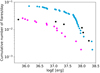 |
Fig. 13 Cumulative flare-frequency diagram for three different phases of the Kepler light curve of KIC 2852961. Blue dots correspond to the FFD for the first period of the Kepler data until BJD = 700 (+2454833), when the rotational modulation shows large amplitudes. The FFD plotted in magenta represents the small amplitude period between BJD = 700 and 1300, while the third FFD in black corresponds to the third part of the light curve after BJD = 1300, when the amplitude increased again. See the text for an explanation. |
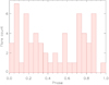 |
Fig. 14 Flare occurence over the rotational phase. The plot indicates no preferred phase for flares. |
9.3 On the flare occurrence along the rotational phase
Since spots and flares are related phenomena, flares are therefore expected to occur when the spotted hemisphere of the star turns in view. In other words, over the rotational phase, more flares occur when more and/or larger spots are in the apparent stellar hemisphere (i.e. at around brightness minima; e.g., Catalano & Frasca 1994; Strassmeier 2000). However, in the bottom panel of Fig. 6, flares seem to occur randomly all over the rotational phase. In Fig. 14 we plotted the rotational phase distribution of the 59 flares. The plot indicates that there is no preferred phases for flare occurrence. According to our K−S test, the phase distribution of flares is random at a 97% significance level. Such a result may be surprising in comparison with the solar case (cf. Guo et al. 2014), but it is not unusual among flaring stars; recent statistical analyses for M dwarf stars (Doyle et al. 2018, 2019) have revealed no indication that flares would occur more frequently at rotational phases around brightness minima. This can partly be understood when considering large starspots (active regions) that cover a much larger fraction of the visible stellar disk compared to sunspots. On stars, flare loops that interconnect distant magnetic regions can be more extended (and more visible) than solar flare loops over bipolar regions. Also, when the inclination angle is not very large, flares could come from spots near the visible pole over the entire rotational phase. For other alternatives, see the discussion in Doyle et al. (2018).
9.4 On the flare energy range, loop size, and statistics
Notsu et al. (2019) discuss the maximum magnetic energy Emag available in a spotted star, which may eventually be converted to flare energy to a certain extent. Here we follow their method to estimate Emag on KIC 2852961. When assuming an appropriate spot temperature, the overall spot coverage of the star (at least the spot coverage difference between the maximum and minimum rotational phases) can be estimated from the relative amplitude of stellar brightness variation. Taking Tspot = 3500 K (cf. Berdyugina 2005) and ΔF∕F ≈ 0.04, maximum relative amplitude from the Kepler light curve plotted in Fig. 4 yields a maximum spot coverage (“spot size”) of L ≈ 0.24 R⋆ (see Eq. (3) in Notsu et al. 2019). Taking L and assuming B = 3.0 kG as a reasonable value of the average magnetic flux density in the spot (cf. Notsu et al. 2019), according to the equation in Shibata & Magara (2011, see their Eq. (1)), the maximum available magnetic energy is estimated to be at least Emag ≈ 3.5 × 1039 erg. However, only a small part of this energy is available to feed a flare because it is distributed as potential field energy. Nevertheless, this rough estimation, which is ≈15 times higher than the highest flare energies in Table 3, is in fair agreement with the observed flare energies of KIC 2852961.
As mentioned in Sect. 9.3, flare loops that interconnect large and distant spotted areas on magnetically active giant stars can be quite extended. A good example is the active giant σ Gem with Teff = 4630 K and R⋆ = 12.3 R⊙, (i.e. very similar to KIC 2852961), and which has a rotation period of 19.6 days (Kővári et al. 2001). Using Extreme Ultraviolet Explorer observations, Mullan et al. (2006) studied the lengths of flaring loops in different types of active stars. Analyzing flares on σ Gem, they found a loop length of 0.85 R* and 80 G as minimum coronal magnetic field strength for a flare lasting 22 h. Starting from this, we can adopt ≈0.5R⋆ as a characteristic flare loop size and assume 100 G as the minimum coronal magnetic field strength (cf. Mullan et al. 2006). According to Namekata et al. (2017, see their Eq. (1)), this would yield at least Emag ≈ 3 × 1039 erg potential energy, which is very similar to the value derived from spot coverage and light curve amplitude in the previous paragraph. This finding suggests that flare loop sizes for the largest flares of KIC 2852961 are indeed on the order of R⋆ (but of course, could be quite different from flare to flare).
Comparing the flare energies of a mixed sample of flares observed on giant stars by Kepler (Yang & Liu 2019) against the flare energies of KIC 2852961, we find that KIC 2852961 flares are more powerful. Both the 35.503 mean and the 35.417 median of the log Ef values in the cited sample of 6842 flares from giant stars are well below our values of 37.286 and 37.384, respectively. Nevertheless, our flare sample is statistically much smaller.
The energy distribution function of KIC 2852961 is plotted in Fig. 15. The histogram exhibits relatively more flares at high energies. Such an excess, however, could be a bias from counting the complex (and thus possibly simultaneous) flares as single ones. Therefore, to see the energy distribution of the regular flares separately, we cleaned the flare sample by excluding the complex events (27 of 59 in Table 3). The histogram of the fraction of regular flares is overplotted in Fig. 15 (in dark red), showing a similar increase at high energies. This supports the idea that the high energy excess in the histogram is not simply an artifact; it seems as if KIC 2852961 may favor the production of superflares. But again, our sample of 59 total flares (of which 32 have a regular shape) is statistically scant, which should also be kept in mind.
9.5 On the scaling effect behind different flare statistics
Ilin et al. (2019) published average slopes of frequency distribution of flare stars in three open clusters (Pleiades, Praesepe, and M67) of different ages (0.125, 0.63, and 4.3 Gyr, respectively) observed by Kepler. The power-law exponents were found to not change with age, and the same was found by Davenport et al. (2019), reflecting a probable universal flare producing mechanism regardless of age (+metallicity, rotational evolution, etc.).
Balona (2015) studied Kepler flare stars of different luminosities and finds that higher luminosity class stars, including giants, generally have higher energy flares. This finding (Balona 2015, see Fig. 10 in that paper) is attributed by the author to a scaling effect; that is to say, in the larger active region of a larger star, more energy can be stored from the same magnetic field strength. Another important finding of Balona (2015) is that stars with lower surface gravities have longer duration flares. Maehara et al. (2015) find that flare duration increases with flare energy, which can be explained by assuming that the time scale of flares emerging from the vicinity of starspots is determined by the characteristic reconnection time (Shibata & Magara 2011). Accordingly, the relationship between Δt and Ef for solar-type main sequence stars is expected to be  . For comparison, we plot logΔt versus log Ef values for KIC 2852961 in Fig. 16. The dots are fitted by a power law in the form of
![Mathematical equation: \begin{equation*} \log \Delta t \textrm{[s]}\,{=}\, -7.30(\pm0.96) + 0.325(\pm0.026)\log E_f \textrm{[erg]}. \end{equation*}](/articles/aa/full_html/2020/09/aa38397-20/aa38397-20-eq15.png) (9)
(9)
We note that fitting only the regular flares (gray dots) or only the complex events (red dots) would yield 0.287 ± 0.032 and 0.361 ± 0.042 slopes, respectively. However, due to small sample sizes, the difference is statistically insignificant. The slope of 0.325 ± 0.026 in Fig. 16is similar to the value of 0.39 ± 0.026 in Maehara et al. (2015) obtained for G-type main sequence stars, supporting the idea that the differences between flare energies are due to size effect (cf. Balona 2015). This scaling idea is echoed by the avalanche models for solar flares, which regard flares as avalanches of many small reconnection events (for an overview, see Charbonneau et al. 2001). This statistical approach could consistently be extended to provide a common framework for solar flares and stellar superflares over many orders of magnitude in energy.
The correlation between spot modulation and flare occurrence presented in Sect. 8 suggests a clear connection between the level of spot activity and the overall flare energy. He et al. (2018) investigated the relationship between the magnetic feature activity and flare activity of three solar-type stars observed by Kepler and conclude that both magnetic feature activity and flare activity are influenced by the same source of magnetic energy (i.e. the magnetic dynamo), similar to the solar case (Hathaway 2015). These are all concordant with the scaling idea from Balona (2015), which says that with larger active regions, more magnetic energy can be stored and thus released by flares (but see also Lehtinen et al. 2020, for a common dynamo scaling in all late-type stars).
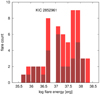 |
Fig. 15 Flare statistics of KIC 2852961. The fraction of the 32 regular flares in the full sample of 59 flares is plotted in dark red. See the text for details. |
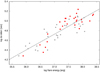 |
Fig. 16 Flare duration vs. flare energy for KIC 2852961 in log–log interpretation. Gray dots are regular flares and red dots indicate the complex events. The fit supports a power-law relationship with a 0.325(±0.026) exponent. |
10 Summary and conclusion
In this paper the flare activity of the late G-early K giant KIC 2852961 was analyzed using the full Kepler data (Q0-Q17) and one TESS light curve (Sector 14 from July-August 2019) in order to study the flare occurrence and other signs of magnetic activity. By adoptingthe Gaia DR-2 parallax, we revised the astrophysical data of the star and derived more reliable parameters, in agreement with the position in the H-R diagram. We found a total of 59 flare events in the Kepler time series and a 60th in the much shorter TESS light curve. Logarithmic flare energies range between 35.74 and 38.38 [erg] (i.e. almost three orders of magnitude);however, the detection cutoff at the low energy end is very likely due to the noise limit. We derived a cumulative FFD diagram, which deviated from a simple power law in the sense that different exponents were obtained for the lower and the higher energy ranges, with a breakpoint between them. We reviewed the possible explanations to understand the broken power law. Flare counts and total flare energies per unit time show temporal variations, which are related to the average light curve amplitude. A straightforward interpretation is that the higher the level of spot activity, the more overall magnetic energy is released by flares and/or superflares. This exciting result supports the assumption that differences in flare (superflare) energies of different luminosity class targets are very likely due to size effect.
Acknowledgements
Authors are grateful to the anonymous referee for his/her valuable comments which helped to improve the manuscript. Authors thank Andrew Vanderburg at Harvard Smithsonian Center for Astrophysics for his help in understanding the action of Presearch Data Conditioning (PDC) module in Kepler data processing. This work was supported by the Hungarian National Research, Development and Innovation Office grant OTKA K131508, KH-130526 and by the Lendület Program of the Hungarian Academy of Sciences, project No. LP2018-7/2019. Authors from Konkoly Observatory acknowledge the financial support of the Austrian-Hungarian Action Foundation (95 öu3, 98öu5, 101öu13). M.N.G. acknowledges support from MIT’s Kavli Institute as a Torres postdoctoral fellow. Data presented in this paper are based on observations obtained with the Hungarian-made Automated Telescope Network, with stations at the Submillimeter Array of the Smithsonian Astrophysical Observatory(SAO), and at the Fred Lawrence Whipple Observatory of SAO. IRAF used in this work was distributed by the National Optical Astronomy Observatory, which was managed by the Association of Universities for Research in Astronomy (AURA) under a cooperative agreement with the National Science Foundation. This research has made use of the NASA Exoplanet Archive, which is operated by the California Institute of Technology, under contract with the National Aeronautics and Space Administration under the Exoplanet Exploration Program. This work presents results from the European Space Agency (ESA) space mission Gaia. Gaia data are being processed by the Gaia Data Processing and Analysis Consortium (DPAC). Funding for the DPAC is provided by national institutions, in particular the institutions participating in the Gaia MultiLateral Agreement (MLA). The Gaia mission website is https://www.cosmos.esa.int/gaia. The Gaia archive website is https://archives.esac.esa.int/gaia.
Appendix A Reliability of the rotational amplitudes
The 30-min. (long-cadence) Kepler photometry is ideal for characterizing short-term signals, such as planetary transits. However, on longer terms of ≈50 days or more, brightness variations such as long-term magnetic activity changes were removed by the processing pipeline. Moreover, Kepler data can also be affected by quarterly systematics, as the instrument was rotated by 90 degrees every three months. Therefore, long-term Kepler data may either obscure true activity-related variability or, on the contrary, mimic false astrophysical signals (see e.g. Kinemuchi et al. 2012). However, long-term variability can be recovered from the FFIs, which were recorded monthly during the primary mission. To recover the long-term brightness variability of KIC 2852961 and to rule out possible unreliable changes, we processed the available FFIs by following the method described in Montet et al. (2017). We used the open-source code f3 provided in that paper, which carries out photometry from the FFIs by centering an appropriate aperture on the given target on every FFI over the primary Kepler mission. The resulting long-term FFI photometry of KIC 2852961 is plotted in Fig. A.1. The plot reflects brightness changes mostly related to the amplitude changes already seen in Fig. 4. However, the monthly sampling of the FFIs is quite close to the 35.5 dayrotation period of the star, which is also markable in the track of the light curve; the frequency of ≈1/200 d−1, seen in the FFI light curve in Fig. A.1, is just an fa alias frequency obtained as the difference between the sampling and data frequencies (i.e. fa = |fd − fs|). Still, the FFI light curve amplitudes are on the order of the light curve amplitudes in Fig. 4 that were obtained by Presearch Data Conditioning (PDC) with simple aperture photometry (SAP), which confirms their reliability.
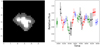 |
Fig. A.1 Kepler FFI photometry of KIC 2852961 obtained using the f3 code from Montet et al. (2017). Left-hand panel: applied original aperture, right-hand panel: FFI light curve. Quarterly changing colors indicate four different positions of the rotated spacecraft (i.e. the CCD). Plotted errors are supposedly instrumental. |
On the other hand, with the exception of the rotation amplitude related variability, no other significant change can be seen over the observing run; in other words, during the four years of the primary Kepler mission, no long-term variability in the overall (average) brightness level of KIC 2852961 can be verified.
References
- Ayres, T. R., Osten, R. A., & Brown, A. 2001, ApJ, 562, L83 [NASA ADS] [CrossRef] [Google Scholar]
- Bakos, G., Noyes, R. W., Kovács, G., et al. 2004, PASP, 116, 266 [NASA ADS] [CrossRef] [Google Scholar]
- Baliunas, S. L., Guinan, E. F., & Dupree, A. K. 1984, ApJ, 282, 733 [NASA ADS] [CrossRef] [Google Scholar]
- Balona, L. A. 2015, MNRAS, 447, 2714 [NASA ADS] [CrossRef] [Google Scholar]
- Balona, L. A., Broomhall, A. M., Kosovichev, A., et al. 2015, MNRAS, 450, 956 [NASA ADS] [CrossRef] [Google Scholar]
- Berdyugina, S. V. 2005, Liv. Rev. Sol. Phys., 2, 8 [Google Scholar]
- Boyajian, T. S., McAlister, H. A., van Belle, G., et al. 2012, ApJ, 746, 101 [NASA ADS] [CrossRef] [Google Scholar]
- Boyajian, T. S., von Braun, K., van Belle, G., et al. 2013, ApJ, 771, 40 [NASA ADS] [CrossRef] [Google Scholar]
- Bressan, A., Marigo, P., Girardi, L., et al. 2012, MNRAS, 427, 127 [NASA ADS] [CrossRef] [Google Scholar]
- Broomhall, A.-M., Davenport, J. R. A., Hayes, L. A., et al. 2019, ApJS, 244, 44 [CrossRef] [Google Scholar]
- Carlberg, J. K., Majewski, S. R., Patterson, R. J., et al. 2011, ApJ, 732, 39 [Google Scholar]
- Catalano, S., & Frasca, A. 1994, A&A, 287, 575 [NASA ADS] [Google Scholar]
- Ceillier, T., Tayar, J., Mathur, S., et al. 2017, A&A, 605, A111 [NASA ADS] [CrossRef] [EDP Sciences] [Google Scholar]
- Charbonneau, P., McIntosh, S. W., Liu, H.-L., & Bogdan, T. J. 2001, Sol. Phys., 203, 321 [Google Scholar]
- Cliver, E. W., & Dietrich, W. F. 2013, J. Space Weather Space Clim., 3, A31 [CrossRef] [EDP Sciences] [Google Scholar]
- Davenport, J. R. A. 2016, ApJ, 829, 23 [Google Scholar]
- Davenport, J. R. A., Hawley, S. L., Hebb, L., et al. 2014, ApJ, 797, 122 [Google Scholar]
- Davenport, J. R. A., Covey, K. R., Clarke, R. W., et al. 2019, ApJ, 871, 241 [Google Scholar]
- Debosscher, J., Blomme, J., Aerts, C., & De Ridder, J. 2011, A&A, 529, A89 [NASA ADS] [CrossRef] [EDP Sciences] [Google Scholar]
- Demircan, O., & Kahraman, G. 1991, Ap&SS, 181, 313 [Google Scholar]
- Doyle, L., Ramsay, G., Doyle, J. G., Wu, K., & Scullion, E. 2018, MNRAS, 480, 2153 [Google Scholar]
- Doyle, L., Ramsay, G., Doyle, J. G., & Wu, K. 2019, MNRAS, 489, 437 [Google Scholar]
- Feinstein, A. D., Montet, B. T., Foreman-Mackey, D., et al. 2019, PASP, 131, 094502 [Google Scholar]
- Ferreira, J. M. 1998, A&A, 335, 248 [NASA ADS] [Google Scholar]
- Flower, P. J. 1996, ApJ, 469, 355 [NASA ADS] [CrossRef] [Google Scholar]
- Gaia Collaboration (Brown, A. G. A., et al.) 2018, A&A, 616, A1 [NASA ADS] [CrossRef] [EDP Sciences] [Google Scholar]
- Gaulme, P., Jackiewicz, J., Spada, F., et al. 2020, A&A, 639, A63 [EDP Sciences] [Google Scholar]
- Gershberg, R. E. 1972, Ap&SS, 19, 75 [Google Scholar]
- Günther, M. N., & Daylan, T. 2019, Astrophysics Source Code Library [record ascl:1903.003] [Google Scholar]
- Günther, M. N., & Daylan, T. 2020, AAS, submitted [arXiv:2003.14371] [Google Scholar]
- Günther, M. N., Zhan, Z., Seager, S., et al. 2020, AJ, 159, 60 [CrossRef] [Google Scholar]
- Guo, J., Lin, J., & Deng, Y. 2014, MNRAS, 441, 2208 [Google Scholar]
- Gustafsson, B., Edvardsson, B., Eriksson, K., et al. 2008, A&A, 486, 951 [NASA ADS] [CrossRef] [EDP Sciences] [Google Scholar]
- Hathaway, D. H. 2015, Liv. Rev. Sol. Phys., 12, 4 [Google Scholar]
- Hawley, S. L., Davenport, J. R. A., Kowalski, A. F., et al. 2014, ApJ, 797, 121 [NASA ADS] [CrossRef] [Google Scholar]
- He, H., Wang, H., Zhang, M., et al. 2018, ApJS, 236, 7 [Google Scholar]
- Howard, W. S., Tilley, M. A., Corbett, H., et al. 2018, ApJ, 860, L30 [Google Scholar]
- Ilin, E., Schmidt, S. J., Davenport, J. R. A., & Strassmeier, K. G. 2019, A&A, 622, A133 [NASA ADS] [CrossRef] [EDP Sciences] [Google Scholar]
- Kasinsky, V. V., & Sotnicova, R. T. 2003, Astron. Astrophys. Trans., 22, 325 [Google Scholar]
- Katsova, M. M., Kitchatinov, L. L., Moss, D., Oláh, K., & Sokoloff, D. D. 2018, Astron. Rep., 62, 513 [Google Scholar]
- Kepler Mission Team. 2009, VizieR Online Data Catalog: V/133 [Google Scholar]
- Kővári, Z s., Strassmeier, K. G., Bartus, J., et al. 2001, A&A, 373, 199 [NASA ADS] [CrossRef] [EDP Sciences] [Google Scholar]
- Kővári, Z s., Künstler, A., Strassmeier, K. G., et al. 2016, A&A, 596, A53 [NASA ADS] [CrossRef] [EDP Sciences] [Google Scholar]
- Kővári, Z s., Oláh, K., Kriskovics, L., et al. 2017a, Astron. Nachr., 338, 903 [Google Scholar]
- Kővári, Z s., Strassmeier, K. G., Carroll, T. A., et al. 2017b, A&A, 606, A42 [NASA ADS] [CrossRef] [EDP Sciences] [Google Scholar]
- Kinemuchi, K., Barclay, T., Fanelli, M., et al. 2012, PASP, 124, 963 [Google Scholar]
- Kretzschmar, M. 2011, A&A, 530, A84 [NASA ADS] [CrossRef] [EDP Sciences] [Google Scholar]
- Kriskovics, L., Kővári, Zs., Vida, K., Granzer, T., & Oláh, K. 2014, A&A, 571, A74 [EDP Sciences] [Google Scholar]
- Kupka, F., Piskunov, N., Ryabchikova, T. A., Stempels, H. C., & Weiss, W. W. 1999, A&AS, 138, 119 [NASA ADS] [CrossRef] [EDP Sciences] [MathSciNet] [PubMed] [Google Scholar]
- Lacy, C. H., Moffett, T. J., & Evans, D. S. 1976, ApJS, 30, 85 [Google Scholar]
- Lehtinen, J. J., Spada, F., Käpylä, M. J., Olspert, N., & Käpylä, P. J. 2020, Nat. Astron., 4, 658 [Google Scholar]
- Leitzinger, M., Odert, P., Greimel, R., et al. 2020, MNRAS, 493, 4570 [Google Scholar]
- Lippiello, E., de Arcangelis, L., & Godano, C. 2008, A&A, 488, L29 [NASA ADS] [CrossRef] [EDP Sciences] [Google Scholar]
- Lomb, N. R. 1976, Ap&SS, 39, 447 [Google Scholar]
- Maehara, H., Shibayama, T., Notsu, S., et al. 2012, Nature, 485, 478 [NASA ADS] [Google Scholar]
- Maehara, H., Shibayama, T., Notsu, Y., et al. 2015, Earth, Planets, and Space, 67, 59 [Google Scholar]
- Maehara, H., Notsu, Y., Notsu, S., et al. 2017, PASJ, 69, 41 [Google Scholar]
- McDonald, I., & Zijlstra, A. A. 2015, MNRAS, 448, 502 [Google Scholar]
- Mihalas, D., & Binney, J. 1981, Galactic astronomy. Structure and kinematics (New York: W.H. Freeman and Company) [Google Scholar]
- Montet, B. T., Tovar, G., & Foreman-Mackey, D. 2017, ApJ, 851, 116 [Google Scholar]
- Mullan, D. J.,& Paudel, R. R. 2018, ApJ, 854, 14 [Google Scholar]
- Mullan, D. J., Mathioudakis, M., Bloomfield, D. S., & Christian, D. J. 2006, ApJS, 164, 173 [Google Scholar]
- Namekata, K., Sakaue, T., Watanabe, K., et al. 2017, ApJ, 851, 91 [Google Scholar]
- Notsu, Y., Maehara, H., Honda, S., et al. 2019, ApJ, 876, 58 [Google Scholar]
- Paudel, R. R., Gizis, J. E., Mullan, D. J., et al. 2018, ApJ, 858, 55 [Google Scholar]
- Pedersen, M. G., Antoci, V., Korhonen, H., et al. 2017, MNRAS, 466, 3060 [Google Scholar]
- Pigulski, A., Pojmański, G., Pilecki, B., & Szczygieł, D. M. 2009, Acta Astron., 59, 33 [NASA ADS] [Google Scholar]
- Piskunov, N., & Valenti, J. A. 2017, A&A, 597, A16 [NASA ADS] [CrossRef] [EDP Sciences] [Google Scholar]
- Pugh, C. E., Armstrong, D. J., Nakariakov, V. M., & Broomhall, A. M. 2016, MNRAS, 459, 3659 [Google Scholar]
- Reinhold, T., & Arlt, R. 2015, A&A, 576, A15 [NASA ADS] [CrossRef] [EDP Sciences] [Google Scholar]
- Roettenbacher, R. M., Monnier, J. D., Korhonen, H., et al. 2016, Nature, 533, 217 [Google Scholar]
- Rubenstein, E. P., & Schaefer, B. E. 2000, ApJ, 529, 1031 [Google Scholar]
- Sanz-Forcada, J., Brickhouse, N. S., & Dupree, A. K. 2002, ApJ, 570, 799 [NASA ADS] [CrossRef] [Google Scholar]
- Scargle, J. D. 1982, ApJ, 263, 835 [Google Scholar]
- Shakhovskaia, N. I. 1989, Sol. Phys., 121, 375 [Google Scholar]
- Shibata, K., & Magara, T. 2011, Liv. Rev. Sol. Phys., 8, 6 [Google Scholar]
- Shibayama, T., Maehara, H., Notsu, S., et al. 2013, ApJS, 209, 5 [Google Scholar]
- Siess, L., & Livio, M. 1999, MNRAS, 308, 1133 [NASA ADS] [CrossRef] [Google Scholar]
- Simon, T., & Drake, S. A. 1989, ApJ, 346, 303 [NASA ADS] [CrossRef] [Google Scholar]
- Skrutskie, M. F., Cutri, R. M., Stiening, R., et al. 2006, AJ, 131, 1163 [NASA ADS] [CrossRef] [Google Scholar]
- Soubiran, C., Jasniewicz, G., Chemin, L., et al. 2018, A&A, 616, A7 [NASA ADS] [CrossRef] [EDP Sciences] [Google Scholar]
- Strassmeier, K. G. 2000, A&A, 357, 608 [NASA ADS] [Google Scholar]
- Strassmeier, K. G., Bartus, J., Kővári, Zs., Weber, M., & Washuettl, A. 1998, A&A, 336, 587 [Google Scholar]
- van Saders, J. L., & Pinsonneault, M. H. 2013, ApJ, 776, 67 [NASA ADS] [CrossRef] [Google Scholar]
- Vida, K., Kővári, Zs., Pál, A., Oláh, K., & Kriskovics, L. 2017, ApJ, 841, 124 [NASA ADS] [CrossRef] [Google Scholar]
- Vida, K., Oláh, K., Kővári, Zs., et al. 2019, ApJ, 884, 160 [NASA ADS] [CrossRef] [Google Scholar]
- Webbink, R. F. 1976, ApJ, 209, 829 [NASA ADS] [CrossRef] [Google Scholar]
- Wheatland, M. S. 2010, ApJ, 710, 1324 [NASA ADS] [CrossRef] [Google Scholar]
- Yang, H., & Liu, J. 2019, ApJS, 241, 29 [CrossRef] [Google Scholar]
- Yashiro, S., Akiyama, S., Gopalswamy, N., & Howard, R. A. 2006, ApJ, 650, L143 [NASA ADS] [CrossRef] [Google Scholar]
- Zinn, J. C., Pinsonneault, M. H., Huber, D., & Stello, D. 2019, ApJ, 878, 136 [NASA ADS] [CrossRef] [Google Scholar]
All Tables
Observing log of the spectroscopic data taken by the Hungarian 1-m RCC telescope.
Peak times (BJD–2 454 833), flare durations, equivalent durations, and flare energies in the Kepler bandpass.
Peak time, duration, equivalent duration, and integrated flare energy in the TESS bandpass for the only flare detected in the TESS Sector 14 data.
All Figures
|
Fig. 1 HATNet photometry of KIC 2852961 collected in one observing season between May and December 2006. Top panel: observationsin I band vs. JD (2,400,000.0+), bottom panel: the folded light curve is plotted using Pphot = 34.27 d period. |
| In the text | |
|
Fig. 2 A large flare of KIC 2852961 on June 26, 2003, observed by HATNet. The slowly changing base light curve shown between June 10 and July 10 covers nearly a whole rotation period. Apart from the flare, the volumes of the nightly changes indicate the overall scatter of the photometric measurements. |
| In the text | |
|
Fig. 3 Radial velocity measurements of KIC 2852961 taken by the 1-m RCC telescope at Piszkéstető Mountain Station, Konkoly Observatory, Hungary, between April 4 and May 3, 2020. |
| In the text | |
|
Fig. 4 Long-cadence Kepler data of KIC 2852961. Note the rotational variability that changes from one rotational cycle to the next,typical for stars with constantly renewing spotted surfaces. Several flare events are also present, including very large ones. |
| In the text | |
|
Fig. 5 Position of KIC 2852961 in the H-R diagram (dot). The stellar evolutionary tracks shown between 1.4 and 2.0 solar masses by 0.2 steps are taken from PARSEC (Bressan et al. 2012), adopting [M/H] = −0.175. From the location, the expected mass is around 1.7 M⊙. |
| In the text | |
|
Fig. 6 Periodogram (top) and folded light curve (bottom) of KIC 2852961 using data shown in Fig. 4. The highest peak of the Lomb-Scargle periodogram indicates a rotation period of ≈35.5 d. Plots are created with the Periodogram Tool of the NASA Exoplanet Archive. |
| In the text | |
|
Fig. 7 Three flares observed on KIC 2852961 with short- and long-cadence in Kepler Q4. Short-cadence data are drawn with a thick blue line, while long-cadence data are overplotted with a thin red line. |
| In the text | |
|
Fig. 8 Two examples for flare detections on KIC 2852961 by Kepler. Top panel: (very likely multiple) flare event of Ef = 2.273 1038 erg energy (Tpeak = 194.634 d in Table 3) with a complex, irregular shape. The superflare of Ef = 1.017 1038 erg shown in the bottom panel (Tpeak = 1330.395 d in Table 3) has a regular light curve. |
| In the text | |
|
Fig. 9 Only flare event on KIC 2852961 found in our TESS Sector 14 data, showing a fairly regular shape; cf. Table 4. |
| In the text | |
|
Fig. 10 Result of the injection-recovery test. Each circle on the plot represents a given model flare characterized by its FWHM and amplitude. The recovery rate of the model flares is represented by a blue gradient bar (the darker the shade, the lower the recovery rate). The energy range in total logarithmic flare energy extends from log E = 33.78 [erg] up to 36.78 [erg], where the recovery rate virtually reaches 100%. |
| In the text | |
|
Fig. 11 Detection bias-corrected cumulative flare-frequency diagram for KIC 2852961. The original detection-biased datapoints are plotted in gray; above them are the corrected points in blue. The fit to the lower energy range below the breakpoint (green line) yields α = 1.29 ± 0.02 parameter, while the fit for the high energy range above the breakpoint (orange line) gives α = 2.84 ± 0.06. |
| In the text | |
|
Fig. 12 Top: moving average of the amplitude of rotational modulation in the Kepler light curve of KIC 2852961 shown in Fig. 4. Bottom: total flare energy within the boxcar of 3Prot used for the moving average. The red tick marks below indicate the peak times of the flare events. See the text for details. |
| In the text | |
|
Fig. 13 Cumulative flare-frequency diagram for three different phases of the Kepler light curve of KIC 2852961. Blue dots correspond to the FFD for the first period of the Kepler data until BJD = 700 (+2454833), when the rotational modulation shows large amplitudes. The FFD plotted in magenta represents the small amplitude period between BJD = 700 and 1300, while the third FFD in black corresponds to the third part of the light curve after BJD = 1300, when the amplitude increased again. See the text for an explanation. |
| In the text | |
|
Fig. 14 Flare occurence over the rotational phase. The plot indicates no preferred phase for flares. |
| In the text | |
|
Fig. 15 Flare statistics of KIC 2852961. The fraction of the 32 regular flares in the full sample of 59 flares is plotted in dark red. See the text for details. |
| In the text | |
|
Fig. 16 Flare duration vs. flare energy for KIC 2852961 in log–log interpretation. Gray dots are regular flares and red dots indicate the complex events. The fit supports a power-law relationship with a 0.325(±0.026) exponent. |
| In the text | |
|
Fig. A.1 Kepler FFI photometry of KIC 2852961 obtained using the f3 code from Montet et al. (2017). Left-hand panel: applied original aperture, right-hand panel: FFI light curve. Quarterly changing colors indicate four different positions of the rotated spacecraft (i.e. the CCD). Plotted errors are supposedly instrumental. |
| In the text | |
Current usage metrics show cumulative count of Article Views (full-text article views including HTML views, PDF and ePub downloads, according to the available data) and Abstracts Views on Vision4Press platform.
Data correspond to usage on the plateform after 2015. The current usage metrics is available 48-96 hours after online publication and is updated daily on week days.
Initial download of the metrics may take a while.