| Issue |
A&A
Volume 641, September 2020
|
|
|---|---|---|
| Article Number | A70 | |
| Number of page(s) | 27 | |
| Section | Extragalactic astronomy | |
| DOI | https://doi.org/10.1051/0004-6361/202038223 | |
| Published online | 10 September 2020 | |
Evidence for supernova feedback sustaining gas turbulence in nearby star-forming galaxies
1
Kapteyn Astronomical Institute, University of Groningen, Landleven 12, 9747 AD Groningen, The Netherlands
e-mail: c.bacchini@rug.nl
2
Dipartimento di Fisica e Astronomia, Università di Bologna, Via Gobetti 93/2, 40129 Bologna, Italy
e-mail: cecilia.bacchini@unibo.it
3
INAF – Osservatorio di Astrofisica e Scienza dello Spazio di Bologna, Via Gobetti 93/3, 40129 Bologna, Italy
4
Dipartimento di Fisica e Astronomia, Università di Padova, Vicolo dell-Osservatorio 3, 35122 Padova, Italy
5
Department of Physics, ETH Zurich, Wolfgang-Pauli-Strasse 27, 8093 Zurich, Switzerland
6
INAF – Osservatorio Astrofisco di Arcetri, Largo E. Fermi 5, 50127 Firenze, Italy
Received:
21
April
2020
Accepted:
16
June
2020
It is widely known that the gas in galaxy discs is highly turbulent, but there is much debate on which mechanism can energetically maintain this turbulence. Among the possible candidates, supernova (SN) explosions are likely the primary drivers but doubts remain on whether they can be sufficient in regions of moderate star formation activity, in particular in the outer parts of discs. Thus, a number of alternative mechanisms have been proposed. In this paper, we measure the SN efficiency η, namely the fraction of the total SN energy needed to sustain turbulence in galaxies, and verify that SNe can indeed be the sole driving mechanism. The key novelty of our approach is that we take into account the increased turbulence dissipation timescale associated with the flaring in outer regions of gaseous discs. We analyse the distribution and kinematics of HI and CO in ten nearby star-forming galaxies to obtain the radial profiles of the kinetic energy per unit area for both the atomic gas and the molecular gas. We use a theoretical model to reproduce the observed energy with the sum of turbulent energy from SNe, as inferred from the observed star formation rate (SFR) surface density, and the gas thermal energy. For the atomic gas, we explore two extreme cases in which the atomic gas is made either of cold neutral medium or warm neutral medium, and the more realistic scenario with a mixture of the two phases. We find that the observed kinetic energy is remarkably well reproduced by our model across the whole extent of the galactic discs, assuming η constant with the galactocentric radius. Taking into account the uncertainties on the SFR surface density and on the atomic gas phase, we obtain that the median SN efficiencies for our sample of galaxies are ⟨ηatom⟩ = 0.015−0.008+0.018 for the atomic gas and ⟨ηmol⟩ = 0.003−0.002+0.006 for the molecular gas. We conclude that SNe alone can sustain gas turbulence in nearby galaxies with only few percent of their energy and that there is essentially no need for any further source of energy.
Key words: galaxies: kinematics and dynamics / galaxies: structure / ISM: kinematics and dynamics / ISM: structure / galaxies: star formation
© ESO 2020
1. Introduction
Gas kinematics provides valuable information about the physical properties of the interstellar medium (ISM). In particular, the velocity dispersion measured from the broadening of emission lines is fundamental for the study of turbulence. Several authors have analysed the kinematics of atomic and molecular gas in nearby star-forming galaxies, finding that the velocity dispersion shows a decreasing trend with the galactocentric radius (e.g. Fraternali et al. 2002; Boomsma et al. 2008; Wilson et al. 2011; Mogotsi et al. 2016; Iorio et al. 2017; Bacchini et al. 2019a). In the inner regions of galaxies, the gas velocity dispersion is typically about 15−20 km s−1, well exceeding the expected broadening due to thermal motions alone (i.e. ≲8 km s−1). This non-thermal broadening is usually ascribed to turbulence. At large galactocentric radii instead (where the molecular gas emission is typically not detected), the velocity dispersion of HI approaches values that are compatible with the thermal broadening of the warm neutral gas (at temperature T ≈ 8000 K).
Both thermal and turbulent motions are forms of disordered energy, but while the first is related to the temperature of the gas particles, the second can be seen as the relative velocity between macroscopic portions of the fluid. The behaviour of turbulence in incompressible fluids is well described by Kolmogorov’s theory (Kolmogorov 1941), which we briefly outline in the following (see e.g. Elmegreen & Scalo 2004 for details). Turbulence entities are envisioned as “eddies” that develop at a variety of different spatial scales. Turbulent energy is injected on a certain scale LD, called driving scale, at which the largest eddies are formed. The largest eddies break down into smaller and smaller eddies and transfer kinetic energy to smaller scales in the so-called “turbulent cascade”, until the dissipation scale ld is reached. The energy is conserved throughout this cascade for any scale between the driving scale and the dissipation scale (i.e. inertial range). At the dissipation scale instead, viscosity transforms the turbulent kinetic energy into internal energy. Kolmogorov’s framework is usually assumed to describe the ISM turbulence, despite the expectation that the gas is compressible in the presence of supersonic turbulent motions (e.g. Elmegreen & Scalo 2004). There are indeed observational indications that Kolmogorov’s theory might be adequate for modelling ISM turbulence (e.g. Elmegreen et al. 2001; Dutta et al. 2009).
Both Kolmogorov’s theory and numerical simulations of compressible supersonic turbulence in the ISM show that the turbulent energy should be rapidly dissipated on timescales of the order of 10 Myr (e.g. Stone et al. 1998; Mac Low et al. 1998; Padoan & Nordlund 1999; Mac Low 1999). Hence, a continuous source of energy is needed in order to maintain the turbulence of the gas ubiquitously observed in galaxies. This issue has stimulated previous research to understand which mechanism is feeding turbulence in galaxies (e.g. Tamburro et al. 2009; Klessen & Hennebelle 2010; Stilp et al. 2013; Utomo et al. 2019). Among the possible candidates, there are different forms of stellar feedback, which include proto-stellar jets, winds from massive stars, ionising radiation, and supernovae (SNe). These latter likely dominate the energy input with respect to the other mechanisms (Mac Low & Klessen 2004; Elmegreen & Scalo 2004). SN explosions are extremely powerful phenomena that can inject a huge amount of energy into the ISM, even though most of this energy is expected to be radiated away (e.g. McKee & Ostriker 1977). Numerical simulation of SN remnant evolution in the ISM have consistently shown that the efficiency of SNe, which is typically defined as the fraction of the total SN energy that is injected into the ISM as kinetic energy, is ∼0.1 (e.g. Thornton et al. 1998; Dib & Burkert 2005; Kim & Ostriker 2015; Martizzi et al. 2016; Fierlinger et al. 2016; Ohlin et al. 2019, but see also Fielding et al. 2018). This appears at odds with a number of recent works showing that the observed kinetic energy of the atomic gas in nearby galaxies requires a SN feedback with a efficiency of ≈0.8 − 1 (e.g. Tamburro et al. 2009; Stilp et al. 2013; Utomo et al. 2019). Therefore, other physical mechanisms have been considered as additional drivers of turbulence, like magneto-rotational instability (MRI, e.g. Sellwood & Balbus 1999), gravitational instability (e.g. Bournaud et al. 2010; Krumholz & Burkhart 2016), rotational shear (e.g. Wada et al. 2002), and accretion flows (e.g. Klessen & Hennebelle 2010; Krumholz & Burkert 2010; Elmegreen & Burkert 2010). However, quantifying the amount of kinetic energy provided by these mechanisms is not straightforward and the values predicted by the models are affected by large uncertainties on the observable quantities (e.g. mass accretion rate, magnetic field intensity). Hence, it is still not clear which (if any) of these additional sources of energy are at play.
A further difficulty in studying the turbulent energy is represented by the challenge of disentangling thermal and turbulent motions in observations. This issue is particularly significant for the atomic gas, which is expected to be present in two phases with different temperatures: the cold neutral medium (CNM) with T ≈ 80 K and the warm neutral medium (WNM) with T ≈ 8000 K (Wolfire et al. 1995, 2003). This latter can significantly contribute to the velocity dispersion (≲8 km s−1) and the kinetic energy, but the lack of information about the relative fraction of CNM and WNM is usually an irksome obstacle to interpreting the observed velocity dispersion. In the Milky Way, Heiles & Troland (2003) estimated that approximately 60% of the atomic hydrogen in the solar neighborhood is WNM (at latitudes larger than 10°; see also Murray et al. 2018). Pineda et al. (2013) found that the fraction of WNM is ∼30% and ∼80% within and beyond the solar radius respectively. However, there are indications of significant variations between galaxies, which stands in the way of adopting the Galactic values for extra-galactic studies. Indeed, Dickey & Brinks (1993) measured that the WNM represents ∼60% and ∼85% of the total HI in M31 and M33, respectively. In the Large Magellanic Cloud, Marx-Zimmer et al. (2000) found that the WNM is about 65%, while Dickey et al. (2000) estimated a lower limit of ∼85% for the Small Magellanic Cloud (see also Jameson et al. 2019). High fractions of WNM were also claimed by Warren et al. (2012), who studied HI line profiles for a sample of 27 nearby galaxies and found that, despite the CNM phase is present in almost all their galaxies, it is only a few percent of the total HI.
The purpose of this work is to understand whether SNe can provide sufficient energy to maintain the turbulence of neutral gas in nearby star-forming galaxies and, in particular, to infer the SN efficiency. The main improvement with respect to previous works is that we take into account the radial flaring of gas discs in galaxies, which implies longer timescales of turbulence dissipation. Moreover, we use a Bayesian method to effectively explore the parameter space of our model of SN-driven turbulence. In this paper, Sect. 2 describes the sample of galaxies and the observations used to measure the kinetic energy. In Sect. 3, we explain how we derive the turbulent energy and the thermal energy components expected from ISM models, and the method used to obtain the SN efficiency from a set of observations. In Sect. 4, we show the resulting profiles of the energy components and provide the SN efficiencies for the galaxies in our sample. In Sect. 5, we derive a “global” value for efficiency of the atomic and the molecular gas by considering the whole sample of galaxies; we then discuss our findings in the broader context of self-regulating star formation and compare our results with previous works in the literature on SN feedback and other driving mechanisms. Section 6 summarises this work and draws our main conclusions.
2. Observations and galaxy sample
Given suitable emission-line spectroscopic observations, the kinetic energy per unit area of the (atomic or molecular) gas in a galaxy as a function of the galactocentric radius, R, can be estimated as
where Σ(R) is the surface density, σ(R) is the velocity dispersion, and the factor of 3 in the first equality comes from the assumption of isotropic velocity dispersion. We calculated Eq. (1) for the neutral gas in a sample of nearby star-forming galaxies by studying the distribution and kinematics of HI and CO, which is adopted as H2 tracer. All the radial profiles used in this work are azimuthal averages calculated by dividing the galaxy into concentric tilted rings of about 400 pc width (see Bacchini et al. 2019a, hereafter B19a).
2.1. Atomic gas distribution and kinematics
In this work, we used the velocity dispersion derived in B19a, in which we studied the HI kinematics in 12 nearby star-forming galaxies using 21 cm emission line data cubes from The HI Nearby Galaxy Survey (THINGS; Walter et al. 2008). The data cubes were analysed using the software 3DBAROLO1 (Di Teodoro & Fraternali 2015), which carries out a tilted-ring model fitting on emission-line data cubes. 3DBAROLO can take into account the beam smearing effect and robustly measure the velocity dispersion and the rotation curve of a galaxy, performing significantly better than 2D methods based on moment maps (e.g. Di Teodoro et al. 2016; Iorio et al. 2017). Figure 2 in B19a shows the radial profiles of the HI velocity dispersion (σHI) for the sample: typically, σHI is 15−20 km s−1 in the inner regions of galaxies and 6−8 km s−1 in the outskirts. For NGC 6946, we performed a new kinematic analysis using the 21-cm data cube in Boomsma et al. (2008) with a spatial resolution of 13″ (i.e. ≈330 pc), as it has an higher signal-to-noise ratio (S/N) with respect to the THINGS data cube used in B19a.
For highly inclined or warped galaxies, the line of sight intercepts regions with different rotation velocity, which can artificially broaden the line profile. This issue biases the velocity dispersion towards high values and 3DBAROLO cannot correct for this effect. Hence, we decided to exclude two galaxies from this study, NGC 2841 (i ≈ 74°) and NGC 7331 (i ≈ 76°), as their average HI velocity dispersion is systematically ≳5 km s−1 above that of the other galaxies. NGC 3198 instead, despite the relatively high inclination (i ≈ 72°), appears much less affected by this issue and is then included in our sample (see Appendix D in B19a for a more detailed discussion). In addition, NGC 5055 shows a warp along the line of sight, which starts beyond R ≈ 10 kpc (Battaglia et al. 2006). In these regions, the velocity dispersion is systematically higher than the typical values in the outer parts of star-forming galaxies, as the line profile is broadened by the merging of emission from different annuli intercepted by the line of sight. Hence, we excluded these regions from this study. We obtained a final sample of eight spiral galaxies and two dwarf galaxies (i.e. DDO 154 and IC 2574).
We derived the HI surface density (ΣHI) as a function of the galactocentric radius with the task ELLPROF of 3DBAROLO, which provides the radial profiles corrected for the galaxy inclination. For NGC 0925, NGC 2403, NGC 3198, and NGC 5055, we used the publicly available data cubes from the Hydrogen Accretion in LOcal GAlaxieS (HALOGAS) Survey (Heald et al. 2011), which have a better S/N with respect to the robust-weighted THINGS data cubes adopted in B19a. DDO 154, IC 2574, NGC 2976, NGC 4736, and NGC 7793 are not included in the HALOGAS sample, hence we obtained ΣHI from the natural-weighted THINGS data cubes, as they have a better S/N with respect to the robust-weighted data cubes. In the case of NGC 6946, we employed the same data cube as in Boomsma et al. (2008). We obtained the surface density of the total atomic gas by accounting for the Helium fraction (ie. Σatom = 1.36ΣHI). We also verified that our profiles are compatible with previous estimates in the literature (Fraternali et al. 2002; Battaglia et al. 2006; Leroy et al. 2008; Boomsma et al. 2008; Bigiel et al. 2010; Gentile et al. 2013; Iorio et al. 2017).
2.2. Molecular gas distribution and kinematics
We measured the velocity dispersion of CO, the typical tracer of the molecular gas, using 3DBAROLO on CO(2–1) emission line data cubes from the HERA CO-Line Extragalactic Survey (HERACLES; Leroy et al. 2005). The emission is detected in seven out of ten galaxies of our sample, except DDO 154, IC 2547, and NGC 7793. We provide the results of the kinematic analysis (e.g. moments maps, position-velocity diagrams, rotation curves) in Appendix A. In B19a, we did not analyse the molecular gas kinematics for each galaxy in the sample, as we relied on previous works in the literature that showed that the velocity dispersion of CO is about half of σHI (Mogotsi et al. 2016; Marasco et al. 2017; Koch et al. 2019). For this work, a robust measurement of the velocity dispersion is desirable to accurately calculate Eq. (1), allowing also to test the assumption used in B19a (see Appendix A). We indicate the molecular gas velocity dispersion with σH2. We must note however that it is not clear whether the nature of the non-thermal component of the molecular gas velocity dispersion is dynamic (i.e. disordered motions between self-gravitating clouds) and hydro-dynamic (i.e. disordered motions between portions of fluid, similarly to the atomic gas turbulence). Our approach based on Kolmogorov’s theory adheres to the second scenario.
We took the radial profiles of the molecular gas surface density (Σmol) from Frank et al. (2016). These authors measured the CO luminosity using HERACLES data cubes and derived Σmol using the CO-to-H2 conversion factor from Sandstrom et al. (2013). These latter authors obtained the radial profile of the conversion factor in a sample of 26 galaxies taking into account the dust-to-gas ratio and the metallicity gradient. NGC 2403 was not included in the study of Sandstrom et al. (2013), hence Frank et al. (2016) adopted the MW value for the conversion factor. The profiles of Frank et al. (2016), which already include the Helium correction, are shown in Fig. 1 in B19a, where the errorbars take into account the uncertainty on the CO-to-H2 conversion factor.
2.3. Star formation rate surface density
To estimate the turbulent energy produced by SNe, we used the observed SFR surface density (ΣSFR). We took as references two different estimates of the SFR surface density, one from Leroy et al. (2008) and Bigiel et al. (2010), and the other from Muñoz-Mateos et al. (2009). This allows us to test the possible dependence of our results on different methods to derive the SFR surface density from the observations.
The profiles from Leroy et al. (2008) are obtained by combining the far-ultraviolet (FUV, i.e. unobscured SF) emission maps from the Galaxy Evolution Explorer (GALEX; Gil de Paz et al. 2007) and the 24 μm (obscured SF) emission maps from the Spitzer Infrared Nearby Galaxy Survey (SINGS; Kennicutt et al. 2003). We also included the profiles from Bigiel et al. (2010), which are derived from FUV GALEX maps out to larger radii with respect to Leroy et al. (2008).
For DDO 154, NGC 2403, NGC 3198, and NGC 6946, ΣSFR(R) is less radially extended than ΣHI(R), as the FUV emission from the outermost radii goes below the sensitivity limit of the observations. In particular, nine out of ten galaxies are in the sample of Bigiel et al. (2010), hence the upper limit on ΣSFR(R) is 2 × 10⁻⁵ M⊙ yr−1 kpc−2. For NGC 6946, which is not included in that study, the upper limit is 10−4 M⊙ yr−1 kpc−2 (Leroy et al. 2008). In our modelling procedure (see Sect. 3), we use these upper limits to constrain the energy injected by SNe at large radii, rather than simply discarding the outskirts of galaxies from our analysis.
To derive a radial profile of SFR surface density from the data of Muñoz-Mateos et al. (2009), we followed the same procedure described in Pezzulli et al. (2015). We adopted the UV extinction radial profiles based on the dust attenuation prescription from Cortese et al. (2008). Among our galaxies, only the dwarf galaxy DDO 154 is not included in this sample. In general, the values of the SFR surface densities derived from Muñoz-Mateos et al. (2009) are above those from Leroy et al. (2008), in particular at large radii, while ΣSFR(R) in the innermost regions of NGC 0925, NGC 3198, and NGC 6946 is reduced. We anticipate that our main conclusions do not change whether we use one or the other determination of the SFR surface density.
3. Methods
In this section, we first describe the energy components that we took into account to estimate theoretically the energy of the atomic gas and the molecular gas. We then explain the method used to compare this energy with the energy profiles calculated from the observations using Eq. (1) in order to obtain the SN efficiency.
3.1. Energy components
We assume that the total energy of the (atomic or molecular) gas per unit area (Emod) is the sum of the turbulent energy (Eturb) and the thermal energy (Eth)

Hence, the velocity dispersion of the gas is
where υturb is the turbulent velocity and υth is the thermal velocity. The equation for the turbulent energy is described below in Sect. 3.1.1 and is the same for the atomic gas and the molecular gas. For the thermal component instead, we discriminate between the atomic and the molecular gas (see Sect. 3.1.2).
3.1.1. Turbulent energy from supernova feedback
The timescale of turbulence dissipation is defined as the ratio between the turbulent energy and its dissipation rate (e.g. Elmegreen & Scalo 2004; Mac Low & Klessen 2004). In the stationary Kolmogorov’s regime, the dissipation rate at the viscosity scale must be equal to the injection rate at the driving scale Ėturb. Therefore, the dissipation timescale can be written as (e.g. Mac Low 1999)
which corresponds to the crossing time of turbulent gas across the driving scale LD (e.g. Elmegreen 2000). This latter is difficult to measure precisely from observations and likely depends on the size of the physical system and the mechanisms under consideration. We note that, as Eqs. (2)–(4) is valid in general for any source of turbulent energy.
This work is focused on SNe, as they are expected to dominate the energy input by stellar feedback on the scale of galactic discs (see Sect. 5.5 for a discussion on other possible sources). We therefore adopted a specific equation to calculate Eturb in Eq. (2) in the case of SNe (i.e. Eturb, SNe). In particular, we assumed that

where h is the scale height of the gas disc, and it is hHI for the atomic gas and hH2 for the molecular gas. This choice is motivated by theoretical models of SN remnant evolution and by observational evidence showing that the explosion of multiple SNe generates expanding shells (super-bubbles), whose diameter can easily reach the thickness of the atomic gas disc (e.g. Mac Low et al. 1989; Boomsma et al. 2008). In addition, LD corresponds to the size of the largest eddies, which are expected to be approximately as large as the physical scale of the system. We discuss in depth the assumption of Eq. (5) in Sect. 5.4.
The gas scale height for each galaxy in our sample was calculated with the same method as in B19a: the gas is assumed in vertical hydrostatic equilibrium in the galactic potential and h is derived iteratively with the Python module GALPYNAMICS2 (Iorio 2018) in order to also take into account the gas self-gravity. The scale height of the gas distribution increases for increasing velocity dispersion σ and for decreasing intensity of the vertical gravitational force gz. Both gz and σ decrease with radius, but the first effect is dominant. Hence, the gas distribution flares with the radius and the scale height increases, reaching hundreds of parsecs in the outer regions of discs. For each galaxy, hHI was calculated for the gravitational potential produced by stars and dark matter (see B19a for details), and then hH2 was derived including also the potential of the atomic gas distribution with the flare3. The radial profiles of hHI for our galaxies can be found in Fig. 4 in B19a. A major improvement of this work is that hH2 was calculated using the velocity dispersion measured from CO data (see Sect. 4.4). We, however, found that the resulting profiles are compatible within the errors with those obtained in B19a, where we assumed σH2 ≈ σHI/2.
Taking NGC 2403 as an example, Fig. 1 shows the dramatic effect of including the flaring of the HI when deriving the dissipation timescale as a function of the galactocentric radius (Eq. (4)). The dashed black line is τd obtained with σHI = 10 km s−1 and hHI = 100 pc, which gives a constant dissipation timescale of 20 Myr. The red curve represents τd(R) calculated with the profiles of hHI(R) and of σHI(R) from B19a. At large radii, the dissipation timescale is prolonged by one order of magnitude with respect to the constant τd. In other words, the observed turbulent energy is easier to maintain in thick discs, even with few SN explosions. We note that the timescale shown in Fig. 1 should be considered a lower limit in the framework of Kolmogorov’s theory, as the observed velocity dispersion used in this example still includes the contribution of thermal motions.
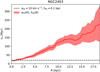 |
Fig. 1. Dissipation timescale of HI turbulence as a function of the galactocentric radius calculated with Eq. (4) for NGC 2403. The dashed black line is τd = 20 Myr obtained with a constant velocity dispersion of 10 km s−1 and a constant scale height of 0.1 kpc (i.e. no flaring). The red curve and band are τd(R) and its uncertainty adopting the radially-decreasing σHI(R) and the increasing hHI(R) from B19a. |
The rate of kinetic energy injection per unit area and per unit time injected by multiple SN explosions is (e.g. Tamburro et al. 2009; Utomo et al. 2019)
where η is the dimensionless efficiency of SNe in transferring kinetic energy to the ISM, ℛcc is the rate of core-collapse SNe per unit area, and ESN = 1051 erg is the total energy released by a single SN. The SN rate per unit area can be obtained from the SFR surface density as
where fcc is the number of core-collapse SNe that explode for unit of stellar mass formed. This latter is  for a Kroupa initial mass function (Kroupa 2002). In Sect. 5.4, we discuss the effect of including type Ia SNe and different parameters for the initial mass function.
The turbulent energy per unit area from SN feedback is obtained from Eq. (4) using Eqs. (5)–(7),
which gives the turbulent energy component in Eq. (2). In Sect. 3.2, we describe how we estimated η for our galaxies using the observational constraints obtained in Sect. 2.
3.1.2. Thermal energy
The thermal velocity in Eq. (3) mainly depends on the temperature of the gas T
where μ is the mean particle weight in units of the proton mass mp and kB is the Boltzmann constant. The mean particle weight varies with the chemical composition of the emitting particles: it is μ ≈ 1 for HI, and μ ≈ 28 for CO. The thermal energy per unit area in Eq. (2) is then
where Σ is the surface density of the gas (atomic or molecular), μ ≈ 1.36 for the atomic gas, and μ ≈ 2.3 for the molecular gas. Thanks to observations and physical models of the ISM, we have useful constraints on the temperature distribution of the atomic gas and the molecular gas in galaxies (see Sects. 4.2 and D.2.2 in Cimatti et al. 2019) and we can estimate the contribution of thermal motions to the observed velocity dispersion.
Atomic gas. The atomic gas is distributed in two phases, CNM and WNM (e.g. Wolfire et al. 1995, 2003; Heiles & Troland 2003), whose contribution to the total thermal velocity depends on their abundance. Let us define fw as the mass fraction of warm atomic gas and label the rest as CNM (with mass fraction 1 − fw). The thermal energy in Eq. (2) is then
![$$ \begin{aligned} E_{\rm th}=E_{\rm th,c} + E_{\rm th,w} = \frac{3}{2} \Sigma _{\rm atom} \left[ \left(1-f_{\rm w} \right) \upsilon _{\rm th,c}^2 + f_{\rm w} \upsilon _{\rm th,w}^2 \right], \end{aligned} $$](/articles/aa/full_html/2020/09/aa38223-20/aa38223-20-eq14.gif)
where Eth, c and Eth, w are the thermal energy of the CNM and the WNM respectively, which can be calculated using Eq. (10) if their temperatures are known. In Eq. (3), we have then
where υth, c and υth, w are given by Eq. (9).
We take as references the average temperatures of the atomic gas resulting from the model by Wolfire et al. (2003, see their Table 3), which are distributed between T ≈ 40 K and T ≈ 190 K for the CNM, and T ≈ 7000 K and T ≈ 8830 K for the WNM. These temperature ranges correspond to 0.6 km s−1 ≲ υth,c ≲ 1.3 km s−1 for the cold HI and 7.6 km s−1 ≲ υth,w ≲ 8.6 km s−1 for the warm HI, respectively. This approach implicitly assumes that the HI is thermally stable, while there are observational indications that ≈50% of the HI in our Galaxy is in the thermally unstable state with T ≈ 500 − 5000 K (Heiles & Troland 2003; Murray et al. 2018). Given these uncertainties, we decided to consider two extreme cases, the first with fw = 0 and the second with fw = 1, which are analysed in Sects. 4.1 and 4.2. Clearly, in these two particular cases, we can directly use Eqs. (9) and (10). This choice allows us to test whether SN feedback can maintain turbulence even with the minimum possible contribution from thermal motions (i.e. CNM case, fw = 0) and to quantify the dependence of our results on the HI temperature distribution. In Sect. 4.3, we investigate the two-phase scenario with 0 < fw < 1 and using Eqs. (11) and (12).
Molecular gas. Molecular gas is observed in giant molecular clouds, where the temperatures are typically very low (T ≈ 10 − 15 K). This gas can be sightly warmer close to young stars (e.g. Redaelli et al. 2017), but the coldest fraction is undoubtedly dominant in mass. We chose 10 K ≲ T ≲ 15 K, which for CO roughly corresponds to υth ≈ 0.06 ± 0.005 km s−1. Hence, thermal motions do not significantly contribute to the observed velocity dispersion (i.e. 5−15 km s−1) for the typical temperatures in molecular clouds.
3.2. Comparison of the model with the observations
In this section, we summarise the method used to infer the SN feedback efficiency required to maintain the turbulent energy in our galaxies. Further details on the formalism of this method can be found in Appendix B.
The algorithm works in the same way for the four cases under consideration: (i) cold atomic gas, (ii) warm atomic gas, (iii) two-phase atomic gas, and (iv) molecular gas (for seven galaxies). We note that the third case involves two free parameters, namely the SN efficiency and the fraction of WNM fw. We assume that the velocity dispersion of the gas is given by the contribution of thermal and turbulent motions (i.e. Eq. (3)), and that turbulence is entirely driven by SNe, implying 0 < η < 1 in Eq. (8). The efficiency is assumed to be constant with the galactocentric radius, but it is allowed to vary from one galaxy to another. The same is for fw in the case of two-phase atomic gas. We adopted a hierarchical Bayesian approach (e.g. Delgado et al. 2019; Cannarozzo et al. 2020; Lamperti et al. 2019) to compare a model for the energy components to the observed profiles.
Bayesian inference is based on the Bayes’ theorem

where p(Θ|𝒟) is the probability distribution of a model depending on a set of parameters Θ given the data 𝒟, p(𝒟|Θ) is the probability distribution of the data given a set of parameters (i.e. the likelihood), and p(Θ) is the prior distribution of the parameters, which includes our a-priori knowledge about their value. The Bayesian approach allows us to take into account the uncertainties on the observed quantities (including the upper limits on ΣSFR), the priors, and the correlation between the model parameters (see for example the case of the two-phase atomic gas in Sect. 4.3). Thus, we obtain a posterior distribution on η which is marginalised over all the other parameters of the model.
Hierarchical methods allow a further level of variability, as the priors on the model parameters depend on an additional set of parameters, the hyper-priors. In other words, the parameters of the priors (Φ) are sampled as the other parameters of the model, assigning them hyper-prior distributions p(Φ). Thus, the Bayes’ rule is written as

where p(Θ|Φ) is the probability distributions of the priors given the hyper-priors. This allows us to parametrise the uncertainty on the priors and use it to obtain robust errors on the final value of η.
In practice, the observed ΣSFR and h4 are considered as realisations of normal distributions centered on unknown true values (i.e.  and hT) and with standard deviation given by the uncertainty on the measurements (i.e. ΔΣSFR and Δh). The true values are assumed to have a log-normal distribution, which depends on priors and hyper-priors (see Appendix B). For any given galaxy,
  and hT are compared with the observed values ΣSFR and h in order to obtain the probability of the observed values given the true values (i.e. the likelihood). For four galaxies in the sample (i.e. DDO 154, NGC 2403, NGC 3198, and NGC 6946), the values of the observed SFR surface density at large radii are upper limits, hence
  is assumed to be a uniform distribution from 0 to the upper limit (see Sect. 2.3).
Similarly, the observed velocity dispersion σ is compared to the distribution of a true velocity dispersion σT to calculate the likelihood probability. In particular, σT is obtained through Eq. (3), which requires to model the thermal and the turbulent velocity components. We have seen in Sect. 3.1.2 that the thermal equilibrium models of the ISM provide useful constraints on the temperature ranges of the gas and the contribution of thermal motions. Hence, we assume that the center and the standard deviation of the thermal velocity distribution are different for the three single-phase cases under consideration: (i) 1 km s−1 and 0.4 km s−1 for the cold atomic gas, (ii) 8.1 km s−1 and 0.5 km s−1 for the warm atomic gas, and (iii) 0.06 km s−1 and 0.005 km s−1 for the molecular gas. For the two-phase case, the thermal velocity is modelled as a uniform distribution between 1 km s−1 and 8.1 km s−1. Our a priori knowledge about the turbulent motions is instead very limited, hence we define  as a log-normal distribution characterised by weakly informative priors and hyper-priors on its centroid velocity and standard deviation (see Appendix B).
A fourth observed quantity, namely the gas surface density Σ, is available to constrain the parameters of our model for the theoretical energy of the gas. We can use  to calculate two useful distributions: (a) the turbulent energy per unit mass
  , and (b) the energy from SNe Eturb, SNe (Eq. (8)). This latter is derived using a uniform prior for η, whose value is between 0 and 1 (see Appendix B). By dividing Eturb, SNe by the density-normalised turbulent energy, we obtain a “prediction” for the gas surface density that can be compared with the observed one, which is modelled as a normal distribution centered on Σ and with standard deviation ΔΣ. From this comparison, we infer the posterior probability of the observed values given this prediction for the surface density.
Finally, we obtain the posterior distribution of η by marginalising over all the other parameters of the model and calculate its median value, whose uncertainty is given by the 16th and the 84th percentiles of the posterior distribution. Henceforth, we refer to this median value as the “best efficiency”. In the case of the two-phase atomic gas, we derive the posterior distribution of fw and its median (i.e. best) value as well. These best values characterise the “best model” in each case under consideration. For each best model, we extract the posterior distributions of Eth, c(R), Eth, w(R), Eth(R), Eturb, SNe(R), and Emod(R) shown in Sect. 4 (see Appendix B), and of  , which is used in Sect. 4.2 to analyse the Mach number in the case of warm atomic gas. The errors on these quantities are calculated as the 16th and the 84th percentile of the posterior distributions. The parameter space is explored with the Hamiltonian Monte Carlo sampler implemented in the Python routine PyMC3 (Hoffman & Gelman 2011; Salvatier et al. 2016).
4. Results
In this section, we present the results of our analysis and focus on the best values of the SN feedback efficiency required to sustain turbulence in the atomic gas and the molecular gas of our sample of galaxies. As already mentioned, we first explore two extreme single-phase cases for the atomic gas, one with CNM only and the other with WNM only, aiming to derive a robust range of values for η. Second, we analyse the more realistic two-phase atomic gas, in which we attempt to derive not only the SN efficiency for each galaxy but also the fraction of WNM. Lastly, we consider the case of the molecular gas. We expect to find different values of η according to the case under consideration, hence we adopt a different nomenclature in each situation: ηatom, c for the CNM, ηatom, w for the WNM, ηatom, 2ph for the 2-phase atomic gas, and ηmol for the molecular gas.
4.1. Cold atomic gas
In the case of all atomic gas in the CNM phase (i.e. fw = 0), thermal motions give the least possible contribution to the total energy and the turbulent energy is dominant. Hence, the efficiency ηatom, c can be seen as an upper limit.
Figure 2 shows, for the galaxies in our sample, the observed energy Eobs (black points, Eq. (1)) and the total kinetic energy Emod of the best model (green area, Eq. (2)) using the SFR surface density from Leroy et al. (2008) and Bigiel et al. (2010). Emod is the sum of the thermal energy Eth, c (blue area, Eq. (10)) and the turbulent energy injected by SNe Eturb, SNe (red area, Eq. (8)). We note that the turbulent energy is two orders of magnitude higher than thermal energy of the CNM at all radii, hence the areas representing Emod(R) and Eturb, SNe(R) tend to overlap. The dotted grey vertical line indicates, for DDO 154, NGC 2403, NGC 3198, and NGC 7793, the outermost radius with measured ΣSFR, hence the upper limit is used for the radii beyond.
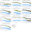 |
Fig. 2. Observed kinetic energy per unit area of the atomic gas (black points) for our sample of galaxies (the errors are calculated with the uncertainty propagation rules applied to Eq. (1)). The blue area shows the thermal energy (Eth, c) of atomic gas if it is assumed to be only CNM. The red area is the turbulent energy injected by SNe (Eturb, SNe) with the efficiency ηatom, c reported on top of each panel. The green area represents the total energy (Emod) calculated as the sum of Eth, c and Eturb, SNe (see Sect. 3.2 and Appendix B). The observed profiles are well reproduced by the theoretical energy for almost all the galaxies. The grey dotted vertical line, when present, indicates the outermost radius with measured ΣSFR, hence the upper limit is used for larger radii. |
The profiles of the observed energy are well reproduced by the theoretical total energy for almost all the galaxies. The efficiencies are ≲0.08 and their median value is ⟨ηatom, c⟩ ≈ 0.035 (see Table 1), showing that SNe with low efficiency can sustain turbulence. However, our model cannot fully reproduce the observed energy in the region 2 kpc ≲ R ≲ 5 kpc of DDO 154 and in the outskirts of IC 2574 and NGC 6946, indicating that some contribution from the thermal energy of the WNM may be required. We stress that the assumption that all the atomic gas is in the form CNM is extreme and unrealistic, so in this case we are underestimating the thermal contribution. Using the SFR surface density from Muñoz-Mateos et al. (2009), we obtain efficiencies that are, on average, a factor of ∼2 lower than the values found using the profiles from Leroy et al. (2008) and the median is indeed ⟨ηatom, c⟩ ≈ 0.015 (see Table 1).
SN feedback efficiency required to sustain turbulence in the neutral gas of our sample of galaxies.
We note that turbulent motions are supersonic in the case of cold atomic gas (i.e. υturb ≫ υth, c). Since the ISM is compressible, supersonic turbulence produces shocks that transform kinetic energy into internal energy, which may also be lost radiatively (see e.g. Tielens 2005, Sect. 11). This would invalidate the energy conservation in the inertial range of the cascade assumed in our model, which is based on the implicit assumption of gas incompressibility in order to apply the Kolmogorov’s theory. In the supersonic regime, our model may be suitable to describe the solenoidal motions, which are incompressible and conserve the energy (Elmegreen & Scalo 2004). In particular, the solenoidal motions are expected to be dominant with respect to the compressible ones (see Sect. 4.4 for further discussion). We recall however that the case of cold atomic gas is unrealistic, hence we may expect that strong shocks have a more limited impact.
4.2. Warm atomic gas
We now consider the case of atomic gas in the warm phase (i.e. WNM), thus the thermal motions give the maximum possible contribution to the total energy. Hence, the efficiency of SN feedback ηatom, w can be considered a lower limit.
The profiles of the observed energy are extremely well reproduced, better than in the previous case for the CNM. In Fig. 3, we show the observed energy and the total energy of the best model using the SFR surface density from Leroy et al. (2008). The main difference with respect to Fig. 2 is that Eturb, SNe dominates only in the inner regions of galaxies, while it is comparable to or lower than Eth, w (orange area) in the other parts. The efficiencies are generally a factor of ∼2 lower than in the case of cold atomic gas and the median value is ⟨ηatom, w⟩ ≈ 0.015 (see Table 1). This indicates that SN feedback with low efficiency can maintain turbulence in the warm atomic gas and that no additional source is required. Using the SFR surface density from Muñoz-Mateos et al. (2009), the resulting efficiencies are lower that those obtained with the other profiles (see Table 1), the median is indeed ⟨ηatom, w⟩ ≈ 0.006.
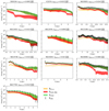 |
Fig. 3. Same as Fig. 2, but the atomic gas is assumed to be only WNM in this case. The orange band shows the thermal energy (Eth, w) and the best efficiency is indicated as ηatom, w. |
In the case of warm atomic gas, it is interesting to analyse the profile of the turbulent velocity in our galaxies to see whether turbulence is supersonic or subsonic. For our sample of galaxies, we calculated the Mach number (ℳ ≡ υturb/υth, w) as a function of the galactocentric radius using the posterior distribution of  obtained from the method described in Sect. 3.2 and the thermal velocity υth, w ≈ 8.1 km s−1. We found that turbulent motions are generally weakly supersonic (i.e. transonic regime): the Mach number typically reaches values of about 2−2.5 only in the innermost regions of spiral galaxies, while it is ℳ ≲ 1 in their outskirts and for dwarf galaxies. The median value is indeed ⟨ℳ⟩ ≈ 1. This suggests that, at least in the transonic regions, adopting Kolmogorov’s theory for incompressible fluids may be acceptable in the case of warm atomic gas.
4.3. Two-phase atomic gas
As already mentioned, both observations and theoretical models of the ISM indicate that the atomic gas is distributed in two phases, CNM and WNM (e.g. Heiles & Troland 2003; Wolfire et al. 2003). Hence, it is interesting to investigate this scenario, as it is more realistic than the single-phase cases seen in Sects. 4.1 and 4.2. We used the same method explained in Sect. 3.2, but the thermal speed and thermal energy are calculated using Eqs. (11) and (12). The thermal speed is the second free parameter in the model and it is used to obtain the WNM fraction fw together with the SN efficiency ηatom, 2ph. This experiment has two possible outcomes: (i) if the observed velocity dispersion is lower than the thermal velocity of the WNM, the posterior distributions for ηatom, 2ph and υth (and therefore fw) will be well constrained and we will calculate the median and the 1σ uncertainty on the best parameters; (ii) if the observed velocity dispersion is higher than the WNM thermal velocity, the best model will tend to be WNM-dominated and equivalent to the case seen in Sect. 4.2. NGC 2403 and NGC 4736, which we discuss below, fall into the former case, while the rest of the galaxies in the sample is compatible with having fw ≈ 1, hence the resulting efficiencies are equivalent to those in Table 1 for the warm atomic gas.
The left panels in Fig. 4 show the result of this analysis for NGC 2403 and NGC 4736: the profiles of the observed energy are remarkably well reproduced by the two-phase best model, for both galaxies. We note that the SN energy is the dominant component in the inner regions, while the total thermal energy (dashed area) tends to become equally significant at large radii, as in the case of warm atomic gas (see Fig. 3). The right panels in Fig. 4 show the corner plots for the ηatom, 2ph and fw, which are obtained from the posterior distribution of υth through Eq. (12). From the 1D and the 2D posterior distributions, we can see that both parameters are well constrained, despite the expected degeneracy. We obtain that the best model is given by ηatom, 2ph ≈ 0.021 and fw ≈ 0.55 (or υth ≈ 6.1 km s−1) for NGC 2403, and ηatom, 2ph ≈ 0.029 and fw ≈ 0.35 (or υth ≈ 4.9 km s−1) for NGC 4736. It is surprising that, despite the unavoidable limitations of our approach, the estimates of the fraction of WNM are compatible with those obtained using different methods for the solar neighborhood (Heiles & Troland 2003), the Milky Way outskirts (Pineda et al. 2013), and the Magellanic Clouds (Marx-Zimmer et al. 2000; Dickey et al. 2000). We note that the best efficiency is compatible within the uncertainties with the value obtained in the WNM-only case. Indeed, we expect that the thermal broadening is dominated by the WNM, even with a fraction of WNM of about 40−60%. It is worth to point out that the uncertainties on ηatom, 2ph should be more reliable than those obtained in the single-phase cases, as the best efficiencies is also marginalised on the thermal speed in this case (as this model takes into account the possible presence of CNM).
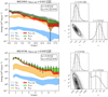 |
Fig. 4. Left panels: observed kinetic energy per unit area of the atomic gas (black points; Eobs from Eq. (1)) for NGC 2403 (upper panel) and NGC 4736 (lower panel). The blue and the orange bands show respectively the thermal energy of the cold (Eth, c) and the warm (Eth, w) atomic gas. The green area is the total kinetic energy predicted by our best model (Emod; see also Appendix B), which includes the total thermal energy (grey dashed area; i.e. Eth from Eq. (11)) and the turbulent energy injected by SN feedback (red area; Eturb, SNe from Eq. (8)) with the best efficiency reported on top of the panel. The grey dotted vertical line indicates the outermost radius of NGC 2403 with measured ΣSFR, the upper limit is used for larger radii. The best fraction of WNM (fw) is reported in the top-right box, together with the corresponding thermal velocity of the atomic gas (Eq. (12)). The observed profile is very well reproduced by the theoretical energy of the best model. Right panels: corner plot showing the marginalised posterior distributions of the SN efficiency and the fraction of WNM fw. The best values with 1σ uncertainties are reported on top of each panel of the 1D posterior distribution. |
We must keep in mind two possible caveats of this analysis. First, we did not include any radial or vertical gradient of the fraction of WNM, which may not be a realistic assumption for some galaxies (e.g. the Milky Way; Pineda et al. 2013, but see Murray et al. 2018 for a different conclusion). We could assume some functional form for fw, linear or exponential trends for instance, but this choice would introduce at least two additional free parameters in the model and worsen the degeneracy issue. The second possible caveat is the assumption that the atomic gas is thermally stable and distributed in CNM and WNM, although there are observational indications that a fraction of the atomic gas may be in the thermally unstable region (e.g. Heiles & Troland 2003; Murray et al. 2018). If we do not assume thermal equilibrium, we can use Eq. (9) and the best υth mentioned above to estimate the temperature of the atomic gas distributed in a single phase. For NGC 2403 and NGC 4736, respectively, we obtain T ≈ 5800 K and T ≈ 3800 K, which both correspond to the thermally unstable regime (Wolfire et al. 2003; Tamburro et al. 2009).
4.4. Molecular gas
Based on the kinematic analysis of CO data cubes (see Appendix A), we know that the velocity dispersion of CO is much higher than the thermal velocity expected for gas with T ≈ 10 − 15 K (i.e. 0.05−0.07 km s−1), indicating strong turbulent motions (e.g. Rosolowsky & Blitz 2005; Sun et al. 2018). This fact allows us to find a very robust estimate for the SN efficiency ηmol.
In Fig. 5, we show the example of NGC 6946, which has an extended molecular gas disc. The profile of the observed energy (black squares) is well reproduced by the theoretical profile Emod with a SN efficiency of about 0.003, except for the points at R ≈ 1.2 kpc and R ≈ 6.4 kpc, which are however uncertain because of the non-circular motions in the innermost regions (see Appendix A) and the low S/N at large radii. As expected, the turbulent energy is fully dominant with respect to the thermal energy (blue area). For the rest of our the sample, Eobs is also very well reproduced by models with ηmol ≲ 0.016, and the median value of the efficiency is ≈0.004 (see Table 1). In Table 1, the shaded rows report the best efficiency values obtained using the SFR surface density from Muñoz-Mateos et al. (2009). In general, the values are lower with respect to those found with the ΣSFR from Leroy et al. (2008), but the two estimates are compatible within the errors.
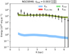 |
Fig. 5. Observed kinetic energy per unit area of the molecular gas (black squares) for NGC 6946. The green area represents the total theoretical energy (Emod; see also Appendix B) calculated as the sum of the thermal energy (blue band; Eth) and the turbulent energy injected by SNe (red band; Eturb, SNe) with the efficiency ηmol reported on top of the panel. Eturb, SNe is indistinguishable from Emod, as the thermal energy contribution is negligible. |
In the case of molecular gas, turbulent motions are strongly supersonic. As mentioned in Sect. 4.1, our model is not suitable to describe this regime, as the energy is not conserved in the turbulent cascade and Kolmogorov’s theory cannot be applied (e.g. Elmegreen & Scalo 2004). Recent numerical simulations of SN-driven supersonic turbulence in molecular clouds suggest that the ratio between compressible and solenoidal motions is about 1/3 − 1/2 (Padoan et al. 2016; Pan et al. 2016; see also Orkisz et al. 2017 for an observational study). We could speculate that, if solenoidal and compressible motions are separable, the SN efficiency obtained with our model should by multiplied by a factor of the order of unity to take into account the kinetic energy dissipated through shocks.
5. Discussion
Our results show that SN feedback can maintain turbulence in the atomic gas of nearby disc galaxies with injection efficiency between 0.003 and 0.077. To drive molecular gas turbulence, the required efficiencies are also low (ηmol ≲ 0.016). Hence, turbulence can be sustained by SNe alone and no other energy sources are required.
5.1. A “global” SN efficiency for nearby galaxies?
We have seen that the values of the best efficiency depend on the choice of the SFR surface density. In the case of the atomic gas, the efficiency depends on the assumed temperature distribution as well. However, finding a single value for the efficiencies may be useful, for example, to include a recipe for SN feedback in numerical simulations and analytical models of galaxy evolution. We can use the posterior distributions of ηatom, c and ηatom, w to obtain this value in the case of the atomic gas (i.e. ⟨ηatom⟩) and those of ηmol for the molecular gas (i.e. ⟨ηmol⟩). For each galaxy, we extracted a random sub-sample of one thousand values from the posterior distributions of the efficiency in each of the cases explored in Sect. 4. For the atomic gas, we have four cases to consider: (i) CNM and (ii) WNM with ΣSFR from Leroy et al. (2008) and Bigiel et al. (2010), and (iii) CNM and (iv) WNM with ΣSFR from Muñoz-Mateos et al. (2009). For the molecular gas, we have only two cases, each with a different ΣSFR. We calculated the median and the 1σ uncertainty using the sub-samples of the posterior distributions, finding  for the atomic gas and
  for the molecular gas.
Figure 6 aims to summarise our findings. The left-hand side concerns the atomic gas and the right-hand side is for the molecular gas. The panels in the top row show the maximum SN energy (i.e. Eq. (8) with η = 1) on the x-axis and the turbulent component of the observed energy (Eobs, turb, i.e. Eq. (1) with the thermal energy subtracted) on the y-axis. To make all the points visible, we do not display the uncertainties and the symbols for the CNM cases are shaded (given that this scenario is also not fully realistic for the atomic gas). The red and the dark red lines show the relations Eobs, turb = ⟨ηatom⟩Eturb, SNe and Eobs, turb = ⟨ηmol⟩Eturb, SNe for the atomic gas and the molecular gas, respectively. The panels in the bottom row show the best efficiencies, as derived with the method described in Sect. 3.2, in comparison with the averages ⟨ηatom⟩ and ⟨ηmol⟩. We can clearly see that, for the atomic gas, efficiencies above 0.1 are not required to sustain the observed turbulent energy. The majority of the points in the top left panel follow the relation with slope ⟨ηatom⟩, indicating that an efficiency of about 0.015 may be a “global” value for the galaxies in our sample. Only a few points belong to the region where η > 0.1, but they correspond to the CNM cases, which are not fully realistic. Similarly, the top right panel shows that the efficiencies for the molecular gas are lower than ∼0.01 for our galaxies and that a possible “global” value is ⟨ηmol⟩ ≈ 0.003. This may suggest that most of the SN energy is transferred to the atomic gas, which is typically the dominant gas phase across the galactic disc.
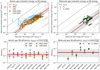 |
Fig. 6. Top row: maximum energy provided by SNe in a dissipation timescale versus the turbulent component of the observed energy, both for the atomic gas (left) and the molecular gas (right). Left panel: the orange points and the blue triangles are respectively for the cases of CNM and of WNM with ΣSFR from Leroy et al. (2008) and Bigiel et al. (2010), while the yellow diamonds and the light blue triangles show the corresponding cases with ΣSFR from Muñoz-Mateos et al. (2009). Each point is for a single galaxy and for a single radius. Right panel: the light green crosses and the green stars are the same quantities for the molecular gas obtained with the two ΣSFR. The red and the dark red lines show the relations built with the “global” efficiencies for the atomic gas ⟨ηatom⟩ and the molecular gas ⟨ηmol⟩ respectively (see text), with grey areas indicating the uncertainty. The solid grey lines show the same relation with efficiencies of 1, while the dotted lines are obtained, from top to bottom, with efficiencies of 0.1, 0.01, 0.001, and 0.0001. Bottom row: summary of the best efficiency for our sample of galaxies, in the case of the atomic (left) and molecular (right) gas. The symbols are the same as in the top row. The red and dark red horizontal lines are the median ⟨ηatom⟩ and ⟨ηmol⟩ (also indicated above each panel) with 1σ error (grey area). Overall, the results of this “global” analysis are consistent with those obtained with the “spatially-resolved” approach, showing that low-efficiency SN feedback can sustain the gas turbulence. |
Theoretical and numerical models of SN explosions in the ISM tend to predict that about 10% of the SN energy is available to feed turbulence (e.g. Chevalier 1974; Thornton et al. 1998; Martizzi et al. 2016; Fierlinger et al. 2016; Ohlin et al. 2019) and some authors have found even higher values (e.g. ≲25%; Dib et al. 2006). A natural question that may arise from our findings considers how the remaining kinetic energy is used. This residual SN energy could be spent to drive large-scale gas motions outside the disc (i.e. galactic fountain, galactic winds, outflows). For example, Fraternali & Binney (2006, 2008) showed that the HI halo of extra-planar gas in NGC 891 and NGC 2403 could be explained with the galactic fountain cycle: a continuous flow of gas launched out of the disc by super-bubble blow-outs. They calculated that this cycle can be sustained with only a small fraction (< 4%) of the SN energy. Marasco et al. (2012) extended these studies to our Galaxy by reproducing the extra-planar HI emission with only ≈0.7% of the kinetic energy from SNe. Moreover, the remaining SN energy could be spent to drive galactic winds (e.g. Fraternali et al. 2004; Veilleux et al. 2005; Rubin et al. 2014; Cresci et al. 2017; Di Teodoro et al. 2018; Armillotta et al. 2019).
5.2. Empirical evidence for the self-regulating cycle of star formation?
Taken at face value, the results presented in this work can be interpreted in a broader context, in which SN feedback and star-formation are key elements of the same self-regulating cycle (see for example Dopita 1985; Ostriker & Shetty 2011). In B19a and Bacchini et al. (2019b), we showed that the SFR volume density correlates with the total gas volume density, following a tight power-law with index ≈2, the volumetric star formation (VSF) law, which is valid for nearby galaxies (both dwarfs and spirals) and the Milky Way. The observed surface densities of the gas and the SFR were converted into volume densities by dividing by the scale height derived under the assumption of hydrostatic equilibrium (same as here). The existence of the VSF law indicates that star formation is regulated by the distribution of the gas, which depends on its velocity dispersion. In this work, we conclude that the turbulent component of the gas velocity dispersion is driven by SN feedback. The energy injected into the ISM by SNe is proportional to the SFR, we can therefore imagine a cycle as follows. If the SFR (per unit volume) increases, the gas becomes more turbulent, implying that the gas disc thickness grows. The gas volume density then decreases and, according to the VSF law, the SFR consequently declines. This can eventually cause the support against the gravitational pull to weaken and the gas volume density to grow again, bringing to a new phase of high SFR. Exploring this self-regulating cycle of star formation and its role in galaxy evolution is of primary interest and we leave it to future work.
5.3. Comparison with previous works on SN feedback
The origin of ISM turbulence has been widely investigated in the literature (see also Sect. 5.5) using different approaches. In this section, we focus on two works that share some similarities with ours.
Tamburro et al. (2009) selected a sample of 11 galaxies (five of them are in our sample as well) and calculated the HI kinetic energy by measuring the surface density and the velocity dispersion using moment maps obtained from the THINGS data cubes. Then, they compared the observed energy with the expected turbulent energy provided by SN feedback (Eq. (8)) and MRI (see discussion in Sect. 5.5.2). In particular, they assumed a constant dissipation timescale of τd = 9.8 Myr (Mac Low 1999) for all the galaxies and constant with radius. They concluded that SN feedback with η ≲ 0.1 can account for the observed kinetic energy in inner parts of the star-forming disc where ΣSFR > 10−3 M⊙ yr−1 kpc−2. In these regions, neither MRI nor thermal motions could explain the observed velocity dispersion of atomic gas. At larger radii instead, they found that unphysical values for the SN efficiency η ≳ 1 are required to maintain the observed line broadening and kinetic energy, given the low SFR (i.e. ΣSFR < 10−3 M⊙ yr−1 kpc−2; see also Stilp et al. 2013). Hence, Tamburro et al. (2009) concluded that the HI velocity dispersion could be driven by the MRI or due to the thermal broadening associated with a warm medium with T ≈ 5000 K. Our results are partially in agreement with Tamburro et al. (2009) concerning the high-SFR regions of galaxies. However, despite we used the same data cubes as Tamburro et al. (2009), we can reproduce the radial profiles of the observed energy per unit area with SN efficiencies ≲0.1 (and no crucial help from thermal motions for most galaxies) not only in the high-SFR regions, but also in the low-SFR ones. The most fundamental difference with respect to this previous work is that we use the scale height of the gas disc to calculate τd, which affects the dissipation timescales (see Fig. 1). Moreover, an important improvement in our work is that we measured the velocity dispersion using a 3D approach, which is more robust than the 2D method based on moment maps adopted by Tamburro et al. (2009). 2D methods perform a Gaussian fit to the line profile in each pixel to measure the line broadening, but this approach can easily fail in pixels with low S/N typical of the outskirts of galaxies. 3DBAROLO, after dividing the galaxy in rings, simultaneously fits the rotation velocity and the azimuthally averaged velocity dispersion in order to minimise the residuals between the data and the model (for each ring). This dramatically improves the velocity dispersion measurement with respect to the pixel-by-pixel fitting of the line profile, even for data with S/N of ≈2 (Di Teodoro & Fraternali 2015).
Recently, Utomo et al. (2019) investigated the origin of turbulence in M33, considering SNe, MRI, and accretion as possible drivers. Using 21 cm and CO(2–1) emission-line data cubes, they studied the kinematic properties and the distribution of atomic gas and clouds of molecular gas. They calculated the dissipation timescale in two ways, using a constant value (i.e. τd = 4.3 Myr) and the second as τd = hHI/σHI, where σHI is the HI velocity dispersion and hHI is the HI scale height calculated assuming the vertical hydrostatic equilibrium (see Ostriker et al. 2010). In the former case, they found that both SN feedback and MRI with efficiencies of 1 are required to maintain turbulence up to R ≈ 8 kpc. In the latter case, the observed turbulence could instead be sustained by SNe and MRI with the efficiency of about 0.1 in the inner regions and 0.6–0.8 beyond R = 6 kpc. Concerning molecular clouds, these authors obtained that the observed turbulent energy could be maintained by SN feedback with 0.001 < η < 0.1. In agreement with Utomo et al. (2019), our results show the importance of calculating the timescale of turbulence dissipation taking into account the increase of the scale height and the radial decrease of the velocity dispersion. The main discrepancy between this previous work and ours is that we conclude that SN feedback alone can maintain turbulence of the atomic gas with efficiencies ≲0.1 (see Fig. 6). There are several differences between this work and ours that may all jointly explain this discrepancy. We discuss below only the two issues with a primary impact on the SN efficiency, as we expect the others to give a secondary contribution (e.g. method to measure σHI, components of the mass model for M33, thermal energy subtraction). First, Utomo et al. (2019) assumed that the energy injected in the ISM by a single SN is ≈3.6 × 1050 erg based on the prescription for the momentum injection by a SN explosion given by Kim & Ostriker (2015), who perfomed numerical simulations of SN explosions in a two-phase medium. Hence, their efficiencies should be multiplied by 0.36 to be compared with ours, reducing the discrepancy. Second, these authors assumed LD = hHI instead of LD = 2hHI, which clearly contributes for another factor of two in the efficiency.
Overall, the main improvement in our work with respect to the literature is that we can explain the observed turbulence with SN feedback only and with a constant efficiency across the galactic discs. The primary reason for our success is that we include the scale height in the calculation of the dissipation timescale. Hence, in contrast with previous authors, we find no indication that other mechanisms are compulsorily required (see Sect. 5.5 for further discussions).
5.4. Possible caveats on the analysis and stability of the results
A possible caveat on this work may be that we considered only the neutral gas components of the ISM, while the ionised gas is also highly turbulent (e.g. Poggianti et al. 2019; Melnick et al. 2019). Within the disc, the ionised gas is typically subdominant in mass with respect to the neutral gas, thus we do not expect that including it would significantly change our conclusions. Some authors investigated the possible sources of the turbulent energy in the ionised gas using the velocity dispersion of Hα emission lines (e.g. Lehnert et al. 2009; Zhou et al. 2017; Yu et al. 2019; Varidel et al. 2020), but it remains unclear whether SN feedback models can reproduce these observations. Taking into account the gas disc flaring probably helps to solve this conundrum, but it is beyond the scope of this work.
The assumption LD = 2h (Eq. (5)) might be questionable. We note however that even adopting LD = h, for instance, our conclusions would not change as the efficiencies would be increased by a factor of 2 only, still being ≲0.1. Our choice is supported by observational as well as theoretical arguments. Analytical and numerical models of the evolution of a SN remnant predict that the shell radius reaches about 100 pc for the typical conditions of the ISM, namely n ≈ 1 − 0.1 cm−3 and σ ≈ 6 − 10 km s−1 (Cox 1972; Chevalier 1974; Chevalier & Gardner 1974; Cioffi et al. 1988; Martizzi et al. 2015, and Sect. 8.7 in Cimatti et al. 2019). However, massive stars are typically found in associations and evolve simultaneously in a small region. These stars produce powerful winds that sweep the ISM from the surroundings, facilitating the expansion of SN shells and generating a super-bubble, that can easily reach the size of the disc thickness and even blow out (Mac Low et al. 1989). Observations of HI holes with diameter of ≈1 kpc in nearby galaxies corroborates this scenario (e.g. Kamphuis et al. 1991; Puche et al. 1992; Boomsma et al. 2008). Given that hHI ≈ 300 − 500 pc (e.g. B19a), our choice of LD = 2hHI is perfectly reasonable. Moreover, in the Small Magellanic Cloud, the velocity power spectrum of atomic gas suggests that LD ≈ 2.3 kpc (Chepurnov et al. 2015), which is consistent with our assumption LD ≈ 2hHI if we adopt hHI ∼ 1 kpc, as indicated by Di Teodoro et al. (2019). The comparison of the observed HI morphology to simulations of dwarf galaxies seems to suggest even higher values (LD ∼ 6 kpc, see Dib & Burkert 2005).
We derived the turbulent energy provided by SNe adopting the prescription for the energy injection rate Ėturb,SNe (Eq. (6)) given by Tamburro et al. (2009), which depends on the SN rate (Eq. (7)). This latter takes into account only core-collapse SNe, as they can be directly related to the recent star formation traced by FUV emission from massive stars younger than 100 Myr (e.g. Kennicutt & Evans 2012). The fraction of SNe Ia is expected to be less than or equal to the fraction of core-collapse SNe depending on the galaxy morphological type (Mannucci et al. 2005; Li et al. 2011). Therefore, considering also SN Ia would not significantly change our results, but just decrease the best values of the efficiencies by a factor ≲2, strengthening our conclusions. The fraction of core-collapse SNe in Eq. (7) also depends on the index and the upper limit on the stellar mass of the initial mass function. We adopted an index of −1.3 for the stars in the mass range between 0.1 M⊙ and 0.5 M⊙, and of −2.3 for those with mass up to 120 M⊙ (Kroupa 2002), which gives  . By decreasing the index or the upper limit on the stellar mass, we would obtain less massive stars and a lower fcc. However, the effect of these variations on the SN efficiency is not straightforward, also the conversion of far-ultraviolet and infrared emission to SFR is affected, but in the opposite direction (i.e. higher SFR for decreasing number of massive stars; see e.g. Tamburro et al. 2009), suggesting that our results are weakly influenced by the initial mass function parameters.
We verified that the general conclusions of this work do not depend on the method used to obtain the best efficiencies that reproduce the observed kinetic energy. In particular, we performed the analysis adopting two additional approaches. The first, which was used to carry out preliminary tests, avoids any fitting procedure and does not involve any assumption on the efficiency. For each galaxy, we simply subtracted, at each galactocentric radius, the expected thermal velocity from the observed velocity dispersion (Eq. (3)) in order to disentangle the turbulent velocity υturb(R). This latter was used to estimate the turbulent energy component, which was then divided by the energy produced by SNe in one turbulent crossing time (i.e. Eq. (8) with η = 1). Thus, we obtained the radial profile of the SN efficiency (i.e. η(R)) without assuming 0 < η < 1, hence the cases with η > 1 were possible. For most of the galaxies, η(R) had large uncertainties (≳50%), in particular at large radii, as the uncertainties on the observable quantities involved in this calculation (e.g. ΣSFR) are larger at large radii than in the inner regions of galaxies (see also Utomo et al. 2019). This indicates that, using this approach, it is not possible to obtain fully satisfactory constraints on the efficiency in the outskirts of galaxies5. For each galaxy, we used η(R) to calculate the median and the 1σ uncertainty and found that these are, albeit very uncertain, grossly compatible with those obtained with the hierarchical method and a constant efficiency. The median values for the whole sample of galaxies are (using ΣSFR from Leroy et al. 2008; Bigiel et al. 2010)  for the cold atomic gas,
  for the warm atomic gas, and
  for the molecular gas. The second approach that we explored is based on the (non-hierarchical) Bayesian framework and consists in fitting Eq. (2) to the observed kinetic energy through the algorithm implemented in the Python module emcee (Foreman-Mackey et al. 2013). We took an efficiency constant with radius as a free parameter with a uniform prior between 0 and 1. The resulting best-fit efficiencies are generally compatible within the errors with those obtained with the hierarchical method. In particular, the median values for the whole sample of galaxies are (using ΣSFR from Leroy et al. 2008; Bigiel et al. 2010)
  for the cold atomic gas,
  for the warm atomic gas, and
  for the molecular gas. We conclude that our results do not depend on the adopted statistical method. The fiducial approach described in Sect. 3.2 is preferable with respect to others, as it offers a rigorous treatment of the uncertainties.
5.5. Other turbulence sources
In this study, we found that SNe are sufficient to maintain the observed turbulence, hence we did not explore in detail other possible sources of energy. Moreover, as we motivate in this section, the contribution from the other drivers is likely of secondary importance and more uncertain than SN feedback.
5.5.1. Other forms of stellar feedback
SNe are not the only form of stellar feedback that can transfer kinetic energy to the ISM (see Mac Low & Klessen 2004; Elmegreen & Scalo 2004, and references therein). Proto-stellar outflows (i.e. jets and winds) can be quite powerful, but they inject energy on scales equal to or smaller than that of molecular cloud complexes. Hence, it seems unlikely that they could feed turbulence on the scale of galactic discs.
O–B and Wolf-Rayet stars also produce strong winds, but only those with the highest masses carry a significant amount of kinetic energy into the ISM. For class O and Wolf-Rayet stars (lifetime ∼4 Myr), the most extreme winds have outflow rates Ṁwind ∼ 10−4 M⊙ yr−1 and velocities Vwind ≈ 3000 km s−1 (e.g. Puls et al. 1996; Nugis & Lamers 2000; Gatto et al. 2017). Winds from less massive stars are typically characterised by Ṁwind ∼ 10−6 M⊙ yr−1 and Vwind ≈ 2000 km s−1 (Puls et al. 1996; Nugis & Lamers 2000), hence their contribution to the ISM turbulence is likely lower, despite the longer lifetimes and higher number of these stars. Gatto et al. (2017) used 3D hydro-dynamic simulations to study the influence of winds and SNe from massive stars on the ISM. They compared the cumulative energy of winds and SN explosions and found that, in the whole wind phase, the most massive stars (≈85 M⊙) produce as much energy as or more energy than in the SN phase. On the other hand, less massive stars (9−20 M⊙) release in the wind phase about 102–104 times less energy than in the SN phase. These less massive stars are much more numerous than the massive ones, thus SN explosions likely dominate over stellar winds after the first few Myr of the stellar population lifetime (Mac Low & Klessen 2004).
A further stellar source of energy is the ionising radiation from massive stars. Most of this energy ionises the diffuse medium around the stars, shaping HII regions and heating the surrounding gas. Ionised gas cools radiatively by emitting non-ionising photons and it contracts due to the thermal instability (see e.g. Cimatti et al. 2019, Sect. 8.1.4), possibly driving turbulent motions. For example, Kritsuk & Norman (2002a,b) estimated that ≲7% of the thermal energy may be converted into kinetic energy through this mechanism. However, as shown by Mac Low & Klessen (2004), the kinetic energy injected into the ISM by ionising radiation is about two to three orders of magnitude lower than produced by SN explosions.
In addition, ionising radiation can transfer kinetic energy to the ISM also through the expansion of HII regions (e.g. Menon et al. 2020). Walch et al. (2012) used 3D SPH simulations to study the effect of the ionising radiation from a single O7 star on a surrounding molecular cloud. They found that ≲0.1% of the ionising energy is converted into kinetic energy and that this form of stellar feedback can sustain turbulent motions of about 2−4 km s−1 (see also Mellema et al. 2006). Overall, these results suggest that, if compared to SNe, the turbulent energy from ionising radiation is of secondary importance.
5.5.2. Magneto-rotational instability and shear
Several authors have proposed that the MRI (Velikhov 1959; Chandrasekhar 1960; Balbus & Hawley 1991) may be the main source of turbulent energy in the outskirts of galaxies, as it generates Maxwell stresses that transfer kinetic energy from shear to the ISM turbulence (e.g. Hawley et al. 1995; Sellwood & Balbus 1999; Piontek & Ostriker 2007). The energy per unit area provided by MRI is (e.g. Mac Low & Klessen 2004; Tamburro et al. 2009; Utomo et al. 2019)
where B is the magnetic field intensity and  is the shear rate in Gyr−1, which depends on the angular frequency Ω ≡ Vrot/R given the rotational velocity of the galaxy Vrot. The energy provided by the MRI can become significant at large radii, hence it has been advocated to explain turbulence in the outskirt of galaxies, in addition to SNe (e.g. Sellwood & Balbus 1999; Tamburro et al. 2009; Utomo et al. 2019). Let us take, for example, NGC 6946, which requires a significant contribution from the thermal energy of the warm atomic gas to explain the observed energy per unit area for R ≳ 10 kpc (see Fig. 3). The ordered magnetic field is B ≈ 5 − 10 μG (Beck 2007), the HI scale heigth grows from hHI ≈ 150 pc at R ≈ 10 kpc to hHI ≈ 180 pc at R ≈ 17 kpc, the rotation curve is approximately constant at about 200 km s−1 for R ≳ 10 kpc, and the turbulent velocity in these regions is also constant at about 5 − 7 km s−1 (see B19a and Boomsma et al. 2008). Using these values in Eq. (15) and assuming ηMRI = 1, we obtain that the MRI can provide Eturb, MRI ≈ 7 − 12 × 1045 erg pc−2 in the regions beyond R ∼ 10 kpc. This estimate of Eturb, MRI is compatible with the observed energy of NGC 6946 (see Fig. 3), but we required that 100% of the MRI energy is transferred to the ISM. For example, non-ideal MHD effects (i.e. Ohmic diffusion, ambipolar diffusion, and Hall effect) can suppress the MRI instability (e.g. Wardle 1999; Kunz & Balbus 2004; Korpi et al. 2010; Riols & Latter 2019). In addition, there are indications that SN driven-turbulence can counteract the MRI in the star-forming regions (e.g. Gressel et al. 2013). We also note that Eturb, MRI calculated with Eq. (15) can be very uncertain. Indeed, the magnetic field intensity is difficult to measure precisely and there are indications that it varies between different regions of a galaxy (e.g. Beck et al. 1996; Beck 2007; Chyży & Buta 2008).
More in general, shear from galactic rotation can transfer kinetic energy to the ISM. It is however not straightforwardly understood how to couple the large scales of galactic rotation to smaller scales and whether the energy input from shear is significant if compared to SN feedback (see e.g. Mac Low & Klessen 2004 and references therein). We conclude that the role of MRI and shear in sustaining the ISM turbulence is still unclear and, given our success in reproducing the observed energy with SNe only, we do not find evidence for the need of these contributions.
5.5.3. Gravitational energy
It has been proposed that turbulence in star-forming galaxies may be driven by gravity through gas accretion (e.g. Klessen & Hennebelle 2010; Elmegreen & Burkert 2010). Klessen & Hennebelle (2010) investigated this mechanism for a sample including the MW and 11 nearby galaxies from the THINGS sample (IC 2547, NGC 4736, NGC 6946, and NGC 7793 are also in our sample). They estimated that the energy input rate from the accreted material (over the whole galaxy) is
where Ṁinfall and Vinfall are the mass inflow rate and the infall speed. For each galaxy, they assumed that Ṁinfall is equal to the observed SFR of the galaxy, based on the idea that gas accretion should sustain star formation. For Vinfall, they used the rotation velocity as an approximation of the impact velocity of the accretion gas onto the galactic disc. Klessen & Hennebelle (2010) calculated the dissipation timescale of turbulence assuming LD = 2hHI and with a equation analogous to Eq. (4). They found that less than 10% of the kinetic energy from accretion is required to sustain turbulence in spiral galaxies (roughly similar with the values in Table 1). On the other hand, they concluded that other energy sources should dominate in dwarf galaxies (e.g. IC 2547), as the expected accretion rate was too low to explain the observed energy.
It is interesting to compare the energy per unit area provided by SN feedback (Eq. (8)) and by accretion (Eturb, infall). This latter can be obtained from Eq. (16) by replacing Ṁinfall with  , and multiplying by the dissipation timescale (Eq. (4)) and the infall efficiency ηinfall (i.e. the fraction of the infall energy that goes into feeding turbulence). Assuming LD = 2hHI, the ratio between the SNe and the infall energies is
where the SN efficiency is defined as ηSNe to distinguish it from the infall efficiency ηinfall. If we take  as suggested by Klessen & Hennebelle (2010), the infall energy is about two orders of magnitude lower than the SN energy when ηinfall ≈ ηSNe. The velocity term in Eq. (17) is unlikely to go in the direction of increasing Eturb, infall/Eturb, SNe. For example, high-velocity clouds, which are among the candidates for accreting gas on to galaxies (e.g. Putman et al. 2012), have velocities between ≈50 km s−1 and ≈150 km s−1 (e.g. Boomsma 2007; Marasco et al. 2013). The galactic fountain cycle is another possible channel for gas accretion, as fountain clouds can trigger gas condensation from the hot corona and fall back onto the disc, bringing new material (see Fraternali et al. 2017 and references therein)6. However, fountain clouds have velocities below 100 km s−1 (e.g. Fraternali & Binney 2006, 2008; Marasco et al. 2012, 2019), hence it is very unlikely that they could transfer a significant amount of energy to the ISM. We also note that
  might vary with the galactocentric radius of galaxies. Marasco et al. (2012) found that the peak in the accretion rate of the galactic fountain lies well beyond the peak of the SFR in the Milky Way. Pezzulli & Fraternali (2016) showed that, in general, this mismatch between the radial profiles of
  and ΣSFR is related to the deficit of angular momentum of the accreted gas with respect to the gas in the disc. Hence, estimating Einfall is not straightforward and requires a careful modelling of the accretion channel under consideration.
Another gravity-driven mechanism that may sustain turbulence is the gravitational instability of the galactic disc, which is usually studied using the Toomre parameter (Toomre 1964). For example, Krumholz & Burkhart (2016) tested two models of turbulence, one based on feedback from star formation and the other on gravitational instability. They compared both models to measurements of the velocity dispersion of HI and Hα lines in both local and distant galaxies, finding that the gravity-driven mode is favoured only in star-forming galaxies with high velocity dispersion (≳50 km s−1) and high SFR (≳10 M⊙ yr−1). This is not the case of our galaxies, which have standard velocity dispersions (about 6−15 km s−1) and star formation rates (i.e. from SFR ≈ 0.005 M⊙ yr−1 for DDO 154 to SFR ≈ 3.2 M⊙ yr−1 for NGC 6946; Leroy et al. 2008). Moreover, whether these high velocity dispersions are real or affected by observational biases is debated. Several authors have shown indeed that, if the effect of beam smearing is properly taken into account, the velocity dispersions in distant galaxies are comparable to or only slightly larger than in local galaxies (e.g. Di Teodoro et al. 2016, 2018; Lelli et al. 2018).
In this work, we have shown that the radial profile of the observed energy can be perfectly reproduced by our simple model of energy injection by SN feedback with constant efficiency. We find no indication that any additional source of energy is required to sustain turbulence in our sample of galaxies. Moreover, the estimates of the energy injected by SNe is the least uncertain considering all the issues related to the other possible driving mechanisms. We conclude that SN feedback is likely the most important driver of turbulence in the ISM of nearby galaxies.
6. Summary and conclusions
The aim of this work is understanding whether SN feedback can sustain turbulence in the atomic gas and the molecular gas of star-forming galaxies. The distribution and kinematics of HI (see Bacchini et al. 2019a) and CO were derived using emission lines data cubes for a sample of ten nearby galaxies, allowing us to calculate the kinetic energy per unit area as a function of the galactocentric radius. We adopted a simple model based on the idea that the gas is in hydrostatic equilibrium and its kinetic energy is given by the sum of two components, namely the turbulent energy and the thermal energy. Relying on Kolmogorov’s framework, we assumed that the turbulent energy is entirely supplied by SN feedback with efficiency η, corresponding to the fraction of the total energy that is transferred to the ISM as kinetic energy. The rate of SN explosions per unit area is derived from the observed SFR surface density. We also assumed that the driving scale of SN feedback is LD = 2h, where h is the scale height of the gas in hydrostatic equilibrium. The increase of the scale height with the galactocentric radius has a crucial impact on the timescale of turbulence dissipation, which is estimated to be one order of magnitude longer at larger radii than in the inner regions of the disc. For the atomic gas in particular, we explored two extreme scenarios with either all CNM or all WNM, in which the thermal motions give respectively the minimum and the maximum possible contribution to the total energy of the gas, and a more realistic case with a mixture of the two phases. We use a Bayesian method to compare our model to a set of observations, aiming to estimate the SN efficiency required to maintain turbulence. We found that the radial profiles of the observed energy per unit area in our sample of galaxies are reproduced by the SN feedback model with η constant with the galactocentric radius at values always below 0.1.
Our main conclusions are the following:
-
At most a few percent of the energy from SN feedback is required to sustain the gas turbulence in our galaxies. We estimate that the median SN efficiency is ⟨ηatom⟩ ≈ 0.015 for the atomic gas and ⟨ηmol⟩ ≈ 0.003 for the molecular gas. Therefore, no additional sources of turbulent energy are needed.
-
Thermal motions significantly contribute to the observed kinetic energy and velocity dispersion of the atomic gas, especially in the outer and low-SFR regions of galaxies.
These findings show that low-efficiency SN feedback is sufficiently energetic to be the sole driver of turbulence in local star-forming galaxies.
The results presented in this work and in Bacchini et al. (2019a,b) provide empirical indications that SN feedback and star formation are part of the same self-regulating cycle (e.g. Dopita 1985; Ostriker & Shetty 2011; Sun et al. 2020). In this scenario, the SFR per unit volume of a galaxy depends on the volume density of the gas as  . The balance between gravity and gas pressure is set by the velocity dispersion of the gas, which includes both thermal and turbulent motions. These latter are sustained by SN feedback and therefore depends on the SFR itself. In future works, we plan to study this self-regulating cycle and its role in galaxy formation and evolution.
In Fig. 3, the black points (Eobs) are sometimes systematically above the green band (Emod) at large radii. This suggests that the best value of the efficiency is slightly more constrained by the inner points, which are less uncertain (i.e. have narrower priors), than those at large radii. However, this is a very minor effect and the model perfectly reproduces Eobs within the uncertainties; even forcing the outer parts to have more weight than the inner ones, the best efficiency would never increase by more than a factor ≲2. Thus, our results strongly point to an efficiency nearly constant with radius.
Fountain clouds return into the disc at approximately the same radius where their were launched in orbit, but with an angular momentum mismatch with respect to the gas in the disc, as they accreted low-angular momentum coronal gas. Therefore, this material is expected to move radially towards the inner and lower-angular momentum regions of the galaxy. In principle, these radial flows could contribute to feeding turbulence. However, Pezzulli & Fraternali (2016) have shown that the radial velocity of this gas is of the order of 1 km s−1, which is negligible with respect to the observed velocity dispersion. Thus, we do not expect radial motions to significantly contribute to turbulence.
Acknowledgments
CB is grateful to E.M. Di Teodoro for the help and the advice in the analysis of the THINGS data cubes. GP acknowledges support by the Swiss National Science Foundation, grant PP00P2_163824. This work was carried out using the publicly available data cubes from HERACLES (Leroy et al. 2005), THINGS (Walter et al. 2008), and HALOGAS (Heald et al. 2011).
References
- Armillotta, L., Krumholz, M. R., Di Teodoro, E. M., & McClure-Griffiths, N. M. 2019, MNRAS, 490, 4401 [NASA ADS] [CrossRef] [Google Scholar]
- Bacchini, C., Fraternali, F., Iorio, G., & Pezzulli, G. 2019a, A&A, 622, A64 [NASA ADS] [CrossRef] [EDP Sciences] [Google Scholar]
- Bacchini, C., Fraternali, F., Pezzulli, G., et al. 2019b, A&A, 632, A127 [NASA ADS] [CrossRef] [EDP Sciences] [Google Scholar]
- Balbus, S. A., & Hawley, J. F. 1991, ApJ, 376, 214 [NASA ADS] [CrossRef] [Google Scholar]
- Battaglia, G., Fraternali, F., Oosterloo, T., & Sancisi, R. 2006, A&A, 447, 49 [NASA ADS] [CrossRef] [EDP Sciences] [Google Scholar]
- Beck, R. 2007, A&A, 470, 539 [NASA ADS] [CrossRef] [EDP Sciences] [Google Scholar]
- Beck, R., Brandenburg, A., Moss, D., Shukurov, A., & Sokoloff, D. 1996, ARA&A, 34, 155 [NASA ADS] [CrossRef] [Google Scholar]
- Bigiel, F., Leroy, A., Walter, F., et al. 2010, AJ, 140, 1194 [NASA ADS] [CrossRef] [Google Scholar]
- Boomsma, R. 2007, PhD Thesis, Kapteyn Astronomical Institute, University of Groningen, The Netherlands [Google Scholar]
- Boomsma, R., Oosterloo, T. A., Fraternali, F., van der Hulst, J. M., & Sancisi, R. 2008, A&A, 490, 555 [NASA ADS] [CrossRef] [EDP Sciences] [Google Scholar]
- Bournaud, F., Elmegreen, B. G., Teyssier, R., Block, D. L., & Puerari, I. 2010, MNRAS, 409, 1088 [NASA ADS] [CrossRef] [Google Scholar]
- Cannarozzo, C., Sonnenfeld, A., & Nipoti, C. 2020, MNRAS, in press [arXiv:1910.06987] [Google Scholar]
- Chandrasekhar, S. 1960, Proc. Natl. Acad. Sci., 46, 253 [NASA ADS] [CrossRef] [Google Scholar]
- Chepurnov, A., Burkhart, B., Lazarian, A., & Stanimirovic, S. 2015, ApJ, 810, 33 [CrossRef] [Google Scholar]
- Chevalier, R. A. 1974, ApJ, 188, 501 [NASA ADS] [CrossRef] [Google Scholar]
- Chevalier, R. A., & Gardner, J. 1974, ApJ, 192, 457 [NASA ADS] [CrossRef] [Google Scholar]
- Chyży, K. T., & Buta, R. J. 2008, ApJ, 677, L17 [NASA ADS] [CrossRef] [Google Scholar]
- Cimatti, A., Fraternali, F., & Nipoti, C. 2019, Introduction to Galaxy Formation and Evolution. From Primordial Gas to Present-day Galaxies (Cambridge: Cambridge University Press) [Google Scholar]
- Cioffi, D. F., McKee, C. F., & Bertschinger, E. 1988, ApJ, 334, 252 [NASA ADS] [CrossRef] [Google Scholar]
- Cortese, L., Boselli, A., Franzetti, P., et al. 2008, MNRAS, 386, 1157 [NASA ADS] [CrossRef] [Google Scholar]
- Cox, D. P. 1972, ApJ, 178, 159 [NASA ADS] [CrossRef] [Google Scholar]
- Cresci, G., Vanzi, L., Telles, E., et al. 2017, A&A, 604, A101 [NASA ADS] [CrossRef] [EDP Sciences] [Google Scholar]
- Delgado, H. E., Sarro, L. M., Clementini, G., Muraveva, T., & Garofalo, A. 2019, A&A, 623, A156 [NASA ADS] [CrossRef] [EDP Sciences] [Google Scholar]
- Di Teodoro, E. M., & Fraternali, F. 2015, MNRAS, 451, 3021 [Google Scholar]
- Di Teodoro, E. M., Fraternali, F., & Miller, S. H. 2016, A&A, 594, A77 [NASA ADS] [CrossRef] [EDP Sciences] [Google Scholar]
- Di Teodoro, E. M., Grillo, C., Fraternali, F., et al. 2018, MNRAS, 476, 804 [CrossRef] [Google Scholar]
- Di Teodoro, E. M., McClure-Griffiths, N. M., Jameson, K. E., et al. 2019, MNRAS, 483, 392 [CrossRef] [Google Scholar]
- Dib, S., & Burkert, A. 2005, ApJ, 630, 238 [NASA ADS] [CrossRef] [Google Scholar]
- Dib, S., Bell, E., & Burkert, A. 2006, ApJ, 638, 797 [NASA ADS] [CrossRef] [Google Scholar]
- Dickey, J. M., & Brinks, E. 1993, ApJ, 405, 153 [NASA ADS] [CrossRef] [Google Scholar]
- Dickey, J. M., Mebold, U., Stanimirovic, S., & Staveley-Smith, L. 2000, ApJ, 536, 756 [NASA ADS] [CrossRef] [Google Scholar]
- Dopita, M. A. 1985, ApJ, 295, L5 [NASA ADS] [CrossRef] [Google Scholar]
- Dutta, P., Begum, A., Bharadwaj, S., & Chengalur, J. N. 2009, MNRAS, 397, L60 [NASA ADS] [Google Scholar]
- Elmegreen, B. G. 2000, ApJ, 530, 277 [NASA ADS] [CrossRef] [Google Scholar]
- Elmegreen, B. G., & Burkert, A. 2010, ApJ, 712, 294 [NASA ADS] [CrossRef] [Google Scholar]
- Elmegreen, B. G., & Scalo, J. 2004, ARA&A, 42, 211 [NASA ADS] [CrossRef] [Google Scholar]
- Elmegreen, B. G., Kim, S., & Staveley-Smith, L. 2001, ApJ, 548, 749 [NASA ADS] [CrossRef] [Google Scholar]
- Fielding, D., Quataert, E., & Martizzi, D. 2018, MNRAS, 481, 3325 [CrossRef] [Google Scholar]
- Fierlinger, K. M., Burkert, A., Ntormousi, E., et al. 2016, MNRAS, 456, 710 [NASA ADS] [CrossRef] [Google Scholar]
- Foreman-Mackey, D., Hogg, D. W., Lang, D., & Goodman, J. 2013, PASP, 125, 306 [CrossRef] [Google Scholar]
- Frank, B. S., de Blok, W. J. G., Walter, F., Leroy, A., & Carignan, C. 2016, AJ, 151, 94 [NASA ADS] [CrossRef] [Google Scholar]
- Fraternali, F. 2017, in Gas Accretion onto Galaxies, eds. A. Fox, & R. Davé, Astrophys. Space Sci. Lib., 430, 323 [NASA ADS] [CrossRef] [Google Scholar]
- Fraternali, F., & Binney, J. J. 2006, MNRAS, 366, 449 [NASA ADS] [CrossRef] [Google Scholar]
- Fraternali, F., & Binney, J. J. 2008, MNRAS, 386, 935 [NASA ADS] [CrossRef] [Google Scholar]
- Fraternali, F., van Moorsel, G., Sancisi, R., & Oosterloo, T. 2002, AJ, 123, 3124 [NASA ADS] [CrossRef] [Google Scholar]
- Fraternali, F., Oosterloo, T., & Sancisi, R. 2004, A&A, 424, 485 [NASA ADS] [CrossRef] [EDP Sciences] [Google Scholar]
- Gatto, A., Walch, S., Naab, T., et al. 2017, MNRAS, 466, 1903 [NASA ADS] [CrossRef] [Google Scholar]
- Gelman, A., Carlin, J. B., Stern, H. S., & Rubin, D. B. 2013, Bayesian Data Analysis, 3rd edn. (Chapman and Hall/CRC) [Google Scholar]
- Gentile, G., Józsa, G. I. G., Serra, P., et al. 2013, A&A, 554, A125 [NASA ADS] [CrossRef] [EDP Sciences] [Google Scholar]
- Gil de Paz, A., Boissier, S., Madore, B. F., et al. 2007, ApJS, 173, 185 [Google Scholar]
- Gressel, O., Elstner, D., & Ziegler, U. 2013, A&A, 560, A93 [NASA ADS] [CrossRef] [EDP Sciences] [Google Scholar]
- Hawley, J. F., Gammie, C. F., & Balbus, S. A. 1995, ApJ, 440, 742 [NASA ADS] [CrossRef] [Google Scholar]
- Heald, G., Józsa, G., Serra, P., et al. 2011, A&A, 526, A118 [NASA ADS] [CrossRef] [EDP Sciences] [Google Scholar]
- Heiles, C., & Troland, T. H. 2003, ApJ, 586, 1067 [NASA ADS] [CrossRef] [Google Scholar]
- Hoffman, M. D., & Gelman, A. 2011, ArXiv e-prints [arXiv:1111.4246] [Google Scholar]
- Iorio, G. 2018, PhD Thesis, University of Bologna, Italy [Google Scholar]
- Iorio, G., Fraternali, F., Nipoti, C., et al. 2017, MNRAS, 466, 4159 [NASA ADS] [Google Scholar]
- Jameson, K. E., McClure-Griffiths, N. M., Liu, B., et al. 2019, ApJS, 244, 7 [CrossRef] [Google Scholar]
- Kamphuis, J., Sancisi, R., & van der Hulst, T. 1991, A&A, 244, L29 [Google Scholar]
- Kennicutt, R. C., & Evans, N. J. 2012, ARA&A, 50, 531 [NASA ADS] [CrossRef] [Google Scholar]
- Kennicutt, R. C., Jr., Armus, L., Bendo, G., et al. 2003, PASP, 115, 928 [NASA ADS] [CrossRef] [Google Scholar]
- Kim, C.-G., & Ostriker, E. C. 2015, ApJ, 802, 99 [NASA ADS] [CrossRef] [Google Scholar]
- Klessen, R. S., & Hennebelle, P. 2010, A&A, 520, A17 [NASA ADS] [CrossRef] [EDP Sciences] [Google Scholar]
- Koch, E. W., Rosolowsky, E. W., Schruba, A., et al. 2019, MNRAS, 485, 2324 [CrossRef] [Google Scholar]
- Kolmogorov, A. 1941, Akademiia Nauk SSSR Doklady, 30, 301 [Google Scholar]
- Korpi, M. J., Käpylä, P. J., & Väisälä, M. S. 2010, Astron. Nachr., 331, 34 [NASA ADS] [CrossRef] [Google Scholar]
- Kritsuk, A. G., & Norman, M. L. 2002a, ApJ, 580, L51 [NASA ADS] [CrossRef] [Google Scholar]
- Kritsuk, A. G., & Norman, M. L. 2002b, ApJ, 569, L127 [NASA ADS] [CrossRef] [Google Scholar]
- Kroupa, P. 2002, Science, 295, 82 [NASA ADS] [CrossRef] [PubMed] [Google Scholar]
- Krumholz, M., & Burkert, A. 2010, ApJ, 724, 895 [CrossRef] [Google Scholar]
- Krumholz, M. R., & Burkhart, B. 2016, MNRAS, 458, 1671 [NASA ADS] [CrossRef] [Google Scholar]
- Kunz, M. W., & Balbus, S. A. 2004, MNRAS, 348, 355 [NASA ADS] [CrossRef] [Google Scholar]
- Lamperti, I., Saintonge, A., De Looze, I., et al. 2019, MNRAS, 489, 4389 [Google Scholar]
- Lehnert, M. D., Nesvadba, N. P. H., Le Tiran, L., et al. 2009, ApJ, 699, 1660 [NASA ADS] [CrossRef] [Google Scholar]
- Lelli, F., De Breuck, C., Falkendal, T., et al. 2018, MNRAS, 479, 5440 [NASA ADS] [CrossRef] [Google Scholar]
- Leroy, A., Bolatto, A. D., Simon, J. D., & Blitz, L. 2005, ApJ, 625, 763 [NASA ADS] [CrossRef] [Google Scholar]
- Leroy, A. K., Walter, F., Brinks, E., et al. 2008, AJ, 136, 2782 [Google Scholar]
- Li, W., Chornock, R., Leaman, J., et al. 2011, MNRAS, 412, 1473 [NASA ADS] [CrossRef] [Google Scholar]
- Mac Low, M.-M. 1999, ApJ, 524, 169 [NASA ADS] [CrossRef] [Google Scholar]
- Mac Low, M.-M., & Klessen, R. S. 2004, Rev. Mod. Phys., 76, 125 [NASA ADS] [CrossRef] [Google Scholar]
- Mac Low, M.-M., McCray, R., & Norman, M. L. 1989, ApJ, 337, 141 [NASA ADS] [CrossRef] [Google Scholar]
- Mac Low, M.-M., Klessen, R. S., Burkert, A., & Smith, M. D. 1998, Phys. Rev. Lett., 80, 2754 [NASA ADS] [CrossRef] [Google Scholar]
- Mannucci, F., Della Valle, M., Panagia, N., et al. 2005, A&A, 433, 807 [NASA ADS] [CrossRef] [EDP Sciences] [Google Scholar]
- Marasco, A., Fraternali, F., & Binney, J. J. 2012, MNRAS, 419, 1107 [NASA ADS] [CrossRef] [Google Scholar]
- Marasco, A., Marinacci, F., & Fraternali, F. 2013, MNRAS, 433, 1634 [NASA ADS] [CrossRef] [Google Scholar]
- Marasco, A., Fraternali, F., van der Hulst, J. M., & Oosterloo, T. 2017, A&A, 607, A106 [NASA ADS] [CrossRef] [EDP Sciences] [Google Scholar]
- Marasco, A., Fraternali, F., Heald, G., et al. 2019, A&A, 631, A50 [NASA ADS] [CrossRef] [EDP Sciences] [Google Scholar]
- Martizzi, D., Faucher-Giguère, C.-A., & Quataert, E. 2015, MNRAS, 450, 504 [NASA ADS] [CrossRef] [Google Scholar]
- Martizzi, D., Fielding, D., Faucher-Giguère, C.-A., & Quataert, E. 2016, MNRAS, 459, 2311 [NASA ADS] [CrossRef] [Google Scholar]
- Marx-Zimmer, M., Herbstmeier, U., Dickey, J. M., et al. 2000, A&A, 354, 787 [NASA ADS] [Google Scholar]
- McKee, C. F., & Ostriker, J. P. 1977, ApJ, 218, 148 [NASA ADS] [CrossRef] [Google Scholar]
- Mellema, G., Arthur, S. J., Henney, W. J., Iliev, I. T., & Shapiro, P. R. 2006, ApJ, 647, 397 [NASA ADS] [CrossRef] [Google Scholar]
- Melnick, J., Terlevich, R., Tenorio-Tagle, G., Telles, E., & Terlevich, E. 2019, A&A, submitted [arXiv:1912.03543] [Google Scholar]
- Menon, S. H., Federrath, C., & Kuiper, R. 2020, MNRAS, 493, 4643 [CrossRef] [Google Scholar]
- Moellenhoff, C., Matthias, M., & Gerhard, O. E. 1995, A&A, 301, 359 [Google Scholar]
- Mogotsi, K. M., de Blok, W. J. G., Caldú-Primo, A., et al. 2016, AJ, 151, 15 [NASA ADS] [CrossRef] [Google Scholar]
- Muñoz-Mateos, J. C., Gil de Paz, A., Boissier, S., et al. 2009, ApJ, 701, 1965 [NASA ADS] [CrossRef] [Google Scholar]
- Murray, C. E., Stanimirović, S., Goss, W. M., et al. 2018, ApJS, 238, 14 [NASA ADS] [CrossRef] [Google Scholar]
- Nugis, T., & Lamers, H. J. G. L. M. 2000, A&A, 360, 227 [NASA ADS] [Google Scholar]
- Ohlin, L., Renaud, F., & Agertz, O. 2019, MNRAS, 485, 3887 [NASA ADS] [CrossRef] [Google Scholar]
- Orkisz, J. H., Pety, J., Gerin, M., et al. 2017, A&A, 599, A99 [NASA ADS] [CrossRef] [EDP Sciences] [Google Scholar]
- Ostriker, E. C., & Shetty, R. 2011, ApJ, 731, 41 [NASA ADS] [CrossRef] [Google Scholar]
- Ostriker, E. C., McKee, C. F., & Leroy, A. K. 2010, ApJ, 721, 975 [NASA ADS] [CrossRef] [Google Scholar]
- Padoan, P., & Nordlund, Å. 1999, ApJ, 526, 279 [NASA ADS] [CrossRef] [Google Scholar]
- Padoan, P., Pan, L., Haugbølle, T., & Nordlund, Å. 2016, ApJ, 822, 11 [NASA ADS] [CrossRef] [Google Scholar]
- Pan, L., Padoan, P., Haugbølle, T., & Nordlund, Å. 2016, ApJ, 825, 30 [NASA ADS] [CrossRef] [Google Scholar]
- Pezzulli, G., & Fraternali, F. 2016, MNRAS, 455, 2308 [NASA ADS] [CrossRef] [Google Scholar]
- Pezzulli, G., Fraternali, F., Boissier, S., & Muñoz-Mateos, J. C. 2015, MNRAS, 451, 2324 [NASA ADS] [CrossRef] [Google Scholar]
- Pineda, J. L., Langer, W. D., Velusamy, T., & Goldsmith, P. F. 2013, A&A, 554, A103 [NASA ADS] [CrossRef] [EDP Sciences] [Google Scholar]
- Piontek, R. A., & Ostriker, E. C. 2007, ApJ, 663, 183 [NASA ADS] [CrossRef] [Google Scholar]
- Pisano, D. J., Wilcots, E. M., & Elmegreen, B. G. 1998, AJ, 115, 975 [NASA ADS] [CrossRef] [Google Scholar]
- Poggianti, B. M., Gullieuszik, M., Tonnesen, S., et al. 2019, MNRAS, 482, 4466 [Google Scholar]
- Puche, D., Westpfahl, D., Brinks, E., & Roy, J.-R. 1992, AJ, 103, 1841 [NASA ADS] [CrossRef] [Google Scholar]
- Puls, J., Kudritzki, R. P., Herrero, A., et al. 1996, A&A, 305, 171 [Google Scholar]
- Putman, M. E., Peek, J. E. G., & Joung, M. R. 2012, ARA&A, 50, 491 [NASA ADS] [CrossRef] [Google Scholar]
- Redaelli, E., Alves, F. O., Caselli, P., et al. 2017, ApJ, 850, 202 [NASA ADS] [CrossRef] [Google Scholar]
- Riols, A., & Latter, H. 2019, MNRAS, 482, 3989 [CrossRef] [Google Scholar]
- Rosolowsky, E., & Blitz, L. 2005, ApJ, 623, 826 [NASA ADS] [CrossRef] [Google Scholar]
- Rubin, K. H. R., Prochaska, J. X., Koo, D. C., et al. 2014, ApJ, 794, 156 [NASA ADS] [CrossRef] [Google Scholar]
- Salvatier, J., Wiecki, T., & Fonnesbeck, C. 2016, PeerJ Comput. Sci., 2, e55 [Google Scholar]
- Sandstrom, K. M., Leroy, A. K., Walter, F., et al. 2013, ApJ, 777, 5 [NASA ADS] [CrossRef] [Google Scholar]
- Sellwood, J. A., & Balbus, S. A. 1999, ApJ, 511, 660 [NASA ADS] [CrossRef] [Google Scholar]
- Stilp, A. M., Dalcanton, J. J., Skillman, E., et al. 2013, ApJ, 773, 88 [NASA ADS] [CrossRef] [Google Scholar]
- Stone, J. M., Ostriker, E. C., & Gammie, C. F. 1998, ApJ, 508, L99 [NASA ADS] [CrossRef] [Google Scholar]
- Sun, J., Leroy, A. K., Schruba, A., et al. 2018, ApJ, 860, 172 [NASA ADS] [CrossRef] [Google Scholar]
- Sun, J., Leroy, A. K., Ostriker, E. C., et al. 2020, ApJ, 892, 148 [CrossRef] [Google Scholar]
- Tamburro, D., Rix, H.-W., Leroy, A. K., et al. 2009, AJ, 137, 4424 [NASA ADS] [CrossRef] [Google Scholar]
- Thornton, K., Gaudlitz, M., Janka, H. T., & Steinmetz, M. 1998, ApJ, 500, 95 [NASA ADS] [CrossRef] [Google Scholar]
- Tielens, A. G. G. M. 2005, The Physics and Chemistry of the Interstellar Medium (Cambridge: Cambridge University Press) [CrossRef] [Google Scholar]
- Toomre, A. 1964, ApJ, 139, 1217 [Google Scholar]
- Utomo, D., Blitz, L., & Falgarone, E. 2019, ApJ, 871, 17 [NASA ADS] [CrossRef] [Google Scholar]
- Varidel, M. R., Croom, S. M., Lewis, G. F., et al. 2020, MNRAS, 495, 2265 [CrossRef] [Google Scholar]
- Veilleux, S., Cecil, G., & Bland-Hawthorn, J. 2005, ARA&A, 43, 769 [Google Scholar]
- Velikhov, E. 1959, Sov. Phys. J. Exp. Theor. Phys., 36, 995 [Google Scholar]
- Wada, K., Meurer, G., & Norman, C. A. 2002, ApJ, 577, 197 [NASA ADS] [CrossRef] [Google Scholar]
- Walch, S. K., Whitworth, A. P., Bisbas, T., Wünsch, R., & Hubber, D. 2012, MNRAS, 427, 625 [NASA ADS] [CrossRef] [Google Scholar]
- Walter, F., Brinks, E., de Blok, W. J. G., et al. 2008, AJ, 136, 2563 [Google Scholar]
- Wardle, M. 1999, MNRAS, 307, 849 [NASA ADS] [CrossRef] [Google Scholar]
- Warren, S. R., Skillman, E. D., Stilp, A. M., et al. 2012, ApJ, 757, 84 [NASA ADS] [CrossRef] [Google Scholar]
- Wilson, C. D., Warren, B. E., Irwin, J., et al. 2011, MNRAS, 410, 1409 [NASA ADS] [Google Scholar]
- Wolfire, M. G., Hollenbach, D., McKee, C. F., Tielens, A. G. G. M., & Bakes, E. L. O. 1995, ApJ, 443, 152 [Google Scholar]
- Wolfire, M. G., McKee, C. F., Hollenbach, D., & Tielens, A. G. G. M. 2003, ApJ, 587, 278 [NASA ADS] [CrossRef] [Google Scholar]
- Yu, X., Shi, Y., Chen, Y., et al. 2019, MNRAS, 486, 4463 [CrossRef] [Google Scholar]
- Zhou, L., Federrath, C., Yuan, T., et al. 2017, MNRAS, 470, 4573 [CrossRef] [Google Scholar]
Appendix A: Detailed molecular gas kinematics
The kinematics of molecular gas was analysed using 3DBAROLO on HERACLES data cubes (see Sect. 2.2), which have a channel separation of 5.2 km s−1 and a spatial resolution of about 13″. We smoothed the data cubes of NGC 2403 to 27″, NGC 2976 to 23″, and NGC 4736 to 18″, in order to match with the working resolution adopted in B19a, and to increase the S/N. The inclination and the position angle were taken from B19a. Small corrections of 2°–3° were applied to NGC 5055 and NGC 6946 after an exploratory fit of the data cube. Indeed, the values reported in B19a were derived from the HI emission, which is more extended than the CO emission, and the inclination and position angle of the outer regions of the HI disc may not be the best choice for the CO disc in the presence of a warp. The systemic velocities are the same as in B19a except for three galaxies, which required a small correction to obtain a better fit the CO data cube: NGC 4736 (+13.3 km s−1), NGC 5055 (+8.3 km s−1), and NGC 6946 (+14.3 km s−1). The panels in Figs. A.1–A.7 provide the main information about the data cubes and the best-fit model of each galaxy7. The description of each panel follows below.
-
Panel A: 0th moment map of CO emission. The white cross indicates the galaxy center and the white ellipse corresponds to the outermost fitted ring.
-
Panel B: velocity field or 1st moment map of the data cube. The thick contour shows the systemic velocity and the black circle in the bottom right corner represents the beam of the telescope or the adopted beam after smoothing, as explained above.
-
Panel C: velocity dispersion map obtained as the 2nd moment map of the data cube. The black bar in the bottom right corner shows the physical scale of the observations.
-
Panel D: molecular gas surface density as a function of the galactocentric radius R from Frank et al. (2016) (see Sect. 2.2 for details).
-
Panel E: rotation velocity as a function of R.
-
Panel F: velocity dispersion radial profile. This is not obtained from the 2nd moment map but through the 3D modelling. The dotted horizontal line shows the velocity resolution limit, which is ≈0.85Δυch ≈ 4.4 km s−1 for Hanning-smoothed data cubes with channel separation Δυch = 5.2 km s−1. The points marked with the red cross (when present) were excluded from this study.
-
Panel G: inclination of the rings, which was kept constant with R (the dashed grey line shows the mean value).
-
Panel H: position angle of the rings. The dashed grey line shows the mean value and the red curve (when present) indicates the regularised profile used to obtain the final model (see Di Teodoro & Fraternali 2015 for details).
-
Panel I: position–velocity diagram along the major axis of the CO disc. The black and the red contours are the iso-density contours of the galaxy and the best-fit model, respectively. The horizontal black dashed line shows the systemic velocity.
-
Panel J: position–velocity diagram along the minor axis.
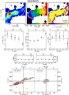 |
Fig. A.1. Moment maps of the data cube of NGC 0925 (panels A, B and C), H2 surface density (panel D), kinematic and geometric properties of the best-fit model (panels E, F, G and H), and position-velocity diagrams (see text for the detailed description). |
From panel F in Figs. A.1–A.7, we can see that the CO velocity dispersion decreases with increasing R, going from 10−20 km s−1 in the inner regions to 4−8 km s−1 at the largest radii, very similar to the HI velocity dispersion profiles obtained by many authors (e.g. Fraternali et al. 2002; Boomsma et al. 2008; Tamburro et al. 2009; Iorio et al. 2017, and B19a). However, the distribution of CO is NGC 0925 and NGC 2976 extends only at R ∼ 2 kpc, hence the decline is not appreciable.
We excluded some points from the analysis, which are indicated with red crosses in the panel F of each galaxy. In particular, the velocity dispersion measured at the outermost radii of most galaxies (i.e. NGC 0925, NGC 3198, NGC 4736, NGC 5055, and NGC 6946) is excluded, as it is lower than the data cubes velocity resolution. From the position-velocity diagrams of NGC 4736 (Fig. A.5) and NGC 6946 (Fig. A.7), we can see that the red contours of 3DBAROLO model are thinner than the black ones of the galaxy emission in the regions within about 1 kpc from the center. This is due to the presence of a bar, which drives strong non-circular motions and produces wiggles in the velocity field (see also Moellenhoff et al. 1995; Boomsma et al. 2008). These kinematic feature cannot be reproduced by the tilted-ring model, as it assumes circular motions. NGC 0925 is also barred galaxy (e.g. Pisano et al. 1998), but in this case the feature is not evident from the position-velocity diagram (Fig. A.1) due to the low S/N of the data. However, the odd shape of the rotation curve suggests that there could be non-circular motions in the region within R ∼ 1 kpc, which cannot be caught by the tilted-ring model. We note that the position angle of NGC 4736 (see panel B in Fig. A.5) is appropriate for the outer disc, while the velocity field in inner regions suggests a lower value. In the case of NGC 6946, we adopted an “ad hoc” approach to improve the model. We first ran 3DBAROLO setting the velocity dispersion at 4 km s−1, in order to retrieve a good-quality rotation curve. Then, we performed a second run fixing the rotation velocities of the rings to those obtained previously, and fitting the velocity dispersion. After inspecting the position-velocity diagram of NGC 6946 (Fig. A.7), we decided however to remove the first two inner points, as the velocity dispersion is clearly overestimated.
Figure A.8 shows, for each galaxy in the sample, the radial profile of the ratio of σCO to σHI. The grey area represents the 84th and the 16th percentile of all the points, which enclose also the median value indicated by the black dash-dotted line ⟨σCO/σHI⟩ = 0.6 ± 0.2. This value is in agreement with previous works (e.g. Mogotsi et al. 2016; Marasco et al. 2017; Koch et al. 2019) and additionally confirms the assumption made in B19a. We note however that the velocity resolution of HERACLES data cubes is not optimal to study the molecular gas velocity dispersion, which may be even lower than 4.4 km s−1 at large radii. Hence, the median value that we found could be slightly overestimated.
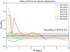 |
Fig. A.8. Ratio of the CO-to-HI velocity dispersion as a function of the galactocentric radius for the galaxies in our sample with CO detected. The median and the 84th and the 16th percentiles are represented by the dot-dashed black line and the grey area, respectively, and their values are reported above. |
Appendix B: Hierarchical Bayesian inference
In this section, we describe the formalism of the Bayesian method presented in Sect. 3.2. We estimate, for each galaxy in our sample, the posterior distribution of η, assuming that it is constant with the galactocentric radius R. For a single galaxy divided in N annuli, the data are  . Let us define RSFR as the outermost radius where the SFR surface density is measured. Hence, we have the upper limit on ΣSFR where Ri > RSFR, which is the case of DDO 154, NGC 2403, NGC 3198, and NGC 6946. For the other galaxies instead, Ri ≤ RSFR at any radius. The observed quantities at a certain radius Ri are therefore

and

The associated uncertainties are

and

As a preliminary step, the observed quantities for each galaxy were normalised to their median value. The elements of di are considered realisation of normal distributions centered on true values (indicated with the apex T) and with standard deviation given by the uncertainties in Δdi. In order to avoid negative true values, we used log-normal distributions as priors (i.e.  ,
,  , and
, and  ). Each log-normal distribution is defined by two parameters: the central value (αυturbi, αΣSFRi, and αhHIi) and the standard deviation (βυturbi, βΣSFRi, and βhHIi), whose hyper-priors are a normal distribution and a Gamma distribution, respectively (see Table B.1). The thermal velocity is a normal distribution with centroid μυth and standard deviation συth of 0.06 km s−1 and 0.005 km s−1 for CO, 1 km s−1 and 0.4 km s−1 for the cold HI, and 8.1 km s−1 and 0.5 km s−1 for the warm HI. The true velocity dispersion is calculated with Eq. (3). Following Sect. 5 in Gelman et al. (2013), the prior on η is defined by a beta-distribution with exponents γη = ϵζ and δη = ζ(1 − ϵ), whose hyper-parameters ϵ and ζ are distributed as reported in Table B.1. Hence, the prior on η is a continuous distribution between 0 and 1, which is equivalent to a uniform distribution in the particular case γη = δη = 1. In addition, this prior of η allows us to explore, at the same time, other distributions than the uniform one, adding a further level of generalisation.
Hyper-priors probability distributions.
Where Ri ≤ RSFR, the likelihood in Eq. (14) is written as
while, where Ri > RSFR, it is
In Eqs. (B.5) and (B.6), the probability distributions of ΣSFRi, σi, hHIi, and ΣHIi are normal distributions. Then, the probability distribution of the priors in Eq. (14), where Ri ≤ RSFR, is
where the probability distributions of  ,
,  ,
,  , and
, and  are log-normal distributions. Where Ri > RSFR, we have instead
and the probability distributions of  is a uniform distribution between 0 and the upper limit uΣSFR.
In the case of the two-phase HI, the probability distribution of the thermal velocity is a uniform distribution between lυth = υth, c = 1 km s−1, which is the value for the CNM, and uυth = υth, w = 8.1 km s−1, which is the value for the WNM.
We note that our best models (green bands in Figs. 2–5) are not directly obtained from Eobs (black points in Figs. 2–5), which is derived through Eq. (1) using the observed velocity dispersion and surface density (the error bars are calculated with the uncertainty propagation rules). As explained in this section and in Sect. 3.2, our procedure is based on the priors on the observable quantities (Eqs. (B.7) and (B.8)). We can define a “true” observed energy ( ) and derive its posterior distribution through Eq. (1) using the priors on Σ and σT. The median and 1σ error of
  are not necessarily the same as the value and the error bar of Eobs. This latter is directly derived from the observed quantities, while
  is “theoretical”. Hence, it is formally correct to compare Emod with Eobs. This specification applies to all the figures shown in Sect. 4.
All Tables
SN feedback efficiency required to sustain turbulence in the neutral gas of our sample of galaxies.
All Figures
|
Fig. 1. Dissipation timescale of HI turbulence as a function of the galactocentric radius calculated with Eq. (4) for NGC 2403. The dashed black line is τd = 20 Myr obtained with a constant velocity dispersion of 10 km s−1 and a constant scale height of 0.1 kpc (i.e. no flaring). The red curve and band are τd(R) and its uncertainty adopting the radially-decreasing σHI(R) and the increasing hHI(R) from B19a. |
| In the text | |
|
Fig. 2. Observed kinetic energy per unit area of the atomic gas (black points) for our sample of galaxies (the errors are calculated with the uncertainty propagation rules applied to Eq. (1)). The blue area shows the thermal energy (Eth, c) of atomic gas if it is assumed to be only CNM. The red area is the turbulent energy injected by SNe (Eturb, SNe) with the efficiency ηatom, c reported on top of each panel. The green area represents the total energy (Emod) calculated as the sum of Eth, c and Eturb, SNe (see Sect. 3.2 and Appendix B). The observed profiles are well reproduced by the theoretical energy for almost all the galaxies. The grey dotted vertical line, when present, indicates the outermost radius with measured ΣSFR, hence the upper limit is used for larger radii. |
| In the text | |
|
Fig. 3. Same as Fig. 2, but the atomic gas is assumed to be only WNM in this case. The orange band shows the thermal energy (Eth, w) and the best efficiency is indicated as ηatom, w. |
| In the text | |
|
Fig. 4. Left panels: observed kinetic energy per unit area of the atomic gas (black points; Eobs from Eq. (1)) for NGC 2403 (upper panel) and NGC 4736 (lower panel). The blue and the orange bands show respectively the thermal energy of the cold (Eth, c) and the warm (Eth, w) atomic gas. The green area is the total kinetic energy predicted by our best model (Emod; see also Appendix B), which includes the total thermal energy (grey dashed area; i.e. Eth from Eq. (11)) and the turbulent energy injected by SN feedback (red area; Eturb, SNe from Eq. (8)) with the best efficiency reported on top of the panel. The grey dotted vertical line indicates the outermost radius of NGC 2403 with measured ΣSFR, the upper limit is used for larger radii. The best fraction of WNM (fw) is reported in the top-right box, together with the corresponding thermal velocity of the atomic gas (Eq. (12)). The observed profile is very well reproduced by the theoretical energy of the best model. Right panels: corner plot showing the marginalised posterior distributions of the SN efficiency and the fraction of WNM fw. The best values with 1σ uncertainties are reported on top of each panel of the 1D posterior distribution. |
| In the text | |
|
Fig. 5. Observed kinetic energy per unit area of the molecular gas (black squares) for NGC 6946. The green area represents the total theoretical energy (Emod; see also Appendix B) calculated as the sum of the thermal energy (blue band; Eth) and the turbulent energy injected by SNe (red band; Eturb, SNe) with the efficiency ηmol reported on top of the panel. Eturb, SNe is indistinguishable from Emod, as the thermal energy contribution is negligible. |
| In the text | |
|
Fig. 6. Top row: maximum energy provided by SNe in a dissipation timescale versus the turbulent component of the observed energy, both for the atomic gas (left) and the molecular gas (right). Left panel: the orange points and the blue triangles are respectively for the cases of CNM and of WNM with ΣSFR from Leroy et al. (2008) and Bigiel et al. (2010), while the yellow diamonds and the light blue triangles show the corresponding cases with ΣSFR from Muñoz-Mateos et al. (2009). Each point is for a single galaxy and for a single radius. Right panel: the light green crosses and the green stars are the same quantities for the molecular gas obtained with the two ΣSFR. The red and the dark red lines show the relations built with the “global” efficiencies for the atomic gas ⟨ηatom⟩ and the molecular gas ⟨ηmol⟩ respectively (see text), with grey areas indicating the uncertainty. The solid grey lines show the same relation with efficiencies of 1, while the dotted lines are obtained, from top to bottom, with efficiencies of 0.1, 0.01, 0.001, and 0.0001. Bottom row: summary of the best efficiency for our sample of galaxies, in the case of the atomic (left) and molecular (right) gas. The symbols are the same as in the top row. The red and dark red horizontal lines are the median ⟨ηatom⟩ and ⟨ηmol⟩ (also indicated above each panel) with 1σ error (grey area). Overall, the results of this “global” analysis are consistent with those obtained with the “spatially-resolved” approach, showing that low-efficiency SN feedback can sustain the gas turbulence. |
| In the text | |
|
Fig. A.1. Moment maps of the data cube of NGC 0925 (panels A, B and C), H2 surface density (panel D), kinematic and geometric properties of the best-fit model (panels E, F, G and H), and position-velocity diagrams (see text for the detailed description). |
| In the text | |
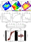 |
Fig. A.2. Same as Fig. A.1 but for NGC 2403. |
| In the text | |
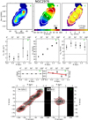 |
Fig. A.3. Same as Fig. A.1 but for NGC 2976. |
| In the text | |
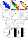 |
Fig. A.4. Same as Fig. A.1 but for NGC 3198. |
| In the text | |
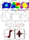 |
Fig. A.5. Same as Fig. A.1 but for NGC 4736. |
| In the text | |
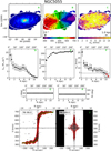 |
Fig. A.6. Same as Fig. A.1 but for NGC 5055. |
| In the text | |
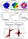 |
Fig. A.7. Same as Fig. A.1 but for NGC 6946. |
| In the text | |
|
Fig. A.8. Ratio of the CO-to-HI velocity dispersion as a function of the galactocentric radius for the galaxies in our sample with CO detected. The median and the 84th and the 16th percentiles are represented by the dot-dashed black line and the grey area, respectively, and their values are reported above. |
| In the text | |
Current usage metrics show cumulative count of Article Views (full-text article views including HTML views, PDF and ePub downloads, according to the available data) and Abstracts Views on Vision4Press platform.
Data correspond to usage on the plateform after 2015. The current usage metrics is available 48-96 hours after online publication and is updated daily on week days.
Initial download of the metrics may take a while.