| Issue |
A&A
Volume 641, September 2020
|
|
|---|---|---|
| Article Number | A129 | |
| Number of page(s) | 16 | |
| Section | Extragalactic astronomy | |
| DOI | https://doi.org/10.1051/0004-6361/202037838 | |
| Published online | 22 September 2020 | |
A high redshift population of galaxies at the North Ecliptic Pole
Unveiling the main sequence of dusty galaxies⋆
1
European Space Astronomy Center, 28691 Villanueva de la Cañada, Spain
e-mail: This email address is being protected from spambots. You need JavaScript enabled to view it.
2
RAL Space, STFC Rutherford Appleton Laboratory, Didcot, Oxfordshire OX11 0QX, UK
3
Oxford Astrophysics, University of Oxford, Keble Rd, Oxford OX1 3RH, UK
4
Department of Physical Sciences, The Open University, Milton Keynes MK7 6AA, UK
5
National Centre for Nuclear Research ul. Pasteura 7, 02-093 Warsaw, Poland
6
Aix Marseille Univ, CNRS, CNES, LAM Marseille, France
7
Dipartimento di Fisica e Astronomia, Università di Padova, Vicolo Osservatorio, 3, 35122 Padova, Italy
8
Astronomy Centre, Department of Physics and Astronomy, University of Sussex, Brighton BN1 9QH, UK
9
Telespazio Vega UK for ESA, European Space Astronomy Centre, Operations Department, 28691 Villanueva de la Cañada, Spain
10
Institute of Space and Astronautical Science, Japan Aerospace Exploration Agency, 3-1-1 Yoshinodai, Chuo, Sagamihara, Kanagawa 252-5210, Japan
11
National Tsing Hua University, No. 101, Section 2, Kuang-Fu Road, Hsinchu, Taiwan 30013
12
Tokyo University of Science, 1-3 Kagurazaka, Shinjuku-ku, Tokyo 162-8601, Japan
13
Department of Physics and Astronomy, UCLA, Los Angeles, CA 90095-1547, USA
14
National Astronomical Observatory, 2-21-1 Osawa, Mitaka, Tokyo, Japan
15
Japan Space Forum, 3-2-1, Kandasurugadai, Chiyoda-ku, Tokyo 101-0062, Japan
16
Department of Astronomy, Kyoto University, Kitashirakawa-Oiwake-cho, Sakyo-ku, Kyoto 606-8502, Japan
17
Academia Sinica Institute of Astronomy and Astrophysics, 11F of Astronomy-Mathematics Building, AS/NTU, No.1, Section 4, Roosevelt Road, Taipei 10617, Taiwan
18
Research Center for Space and Cosmic Evolution, Ehime University, 2-Bunkyo-cho, Matsuyama, Ehime 790-8577, Japan
19
Instituto de Astronomıia sede Ensenada Universidad Nacional Autonoma de Mexico Km 107, Carret. Tij.-Ens., Ensenada, 22060 BC, Mexico
Received:
27
February
2020
Accepted:
3
July
2020
Abstract
Context. Dusty high-z galaxies are extreme objects with high star formation rates (SFRs) and luminosities. Characterising the properties of this population and analysing their evolution over cosmic time is key to understanding galaxy evolution in the early Universe.
Aims. We select a sample of high-z dusty star-forming galaxies (DSFGs) and evaluate their position on the main sequence (MS) of star-forming galaxies, the well-known correlation between stellar mass and SFR. We aim to understand the causes of their high star formation and quantify the percentage of DSFGs that lie above the MS.
Methods. We adopted a multi-wavelength approach with data from optical to submillimetre wavelengths from surveys at the North Ecliptic Pole to study a submillimetre sample of high-redshift galaxies. Two submillimetre selection methods were used, including: sources selected at 850 μm with the Sub-millimetre Common-User Bolometer Array 2) SCUBA-2 instrument and Herschel-Spectral and Photometric Imaging Receiver (SPIRE) selected sources (colour-colour diagrams and 500 μm risers), finding that 185 have good multi-wavelength coverage. The resulting sample of 185 high-z candidates was further studied by spectral energy distribution fitting with the CIGALE fitting code. We derived photometric redshifts, stellar masses, SFRs, and additional physical parameters, such as the infrared luminosity and active galactic nuclei (AGN) contribution.
Results. We find that the Herschel-SPIRE selected DSFGs generally have higher redshifts (z = 2.57−0.09+0.08) than sources that are selected solely by the SCUBA-2 method (z = 1.45−0.06+0.21). We find moderate SFRs (797−50+108 M⊙ yr−1), which are typically lower than those found in other studies. We find that the different results in the literature are, only in part, due to selection effects, as even in the most extreme cases, SFRs are still lower than a few thousand solar masses per year. The difference in measured SFRs affects the position of DSFGs on the MS of galaxies; most of the DSFGs lie on the MS (60%). Finally, we find that the star formation efficiency (SFE) depends on the epoch and intensity of the star formation burst in the galaxy; the later the burst, the more intense the star formation. We discuss whether the higher SFEs in DSFGs could be due to mergers.
Key words: galaxies: evolution / galaxies: high-redshift / galaxies: starburst / submillimeter: galaxies
A table of the multi-wavelength photometry is only available at the CDS via anonymous ftp to cdsarc.u-strasbg.fr (130.79.128.5) or via http://cdsarc.u-strasbg.fr/viz-bin/cat/J/A+A/641/A129
© ESO 2020
1. Introduction
Submillimetre galaxies (SMGs) are amongst the most luminous dusty galaxies in the Universe (Wilkinson et al. 2017). The discovery of this population of bright sources at submillimetre wavelengths (flux densities F850 μm > 2−5 mJy), which is mostly made up of high-z galaxies (z > 1), posed critical questions about the evolution of galaxies in the early Universe (e.g. Barger et al. 1998; Smail et al. 1997; Hughes et al. 1998).
The launch of the Herschel Space Observatory (Pilbratt et al. 2010) and the observations with the Spectral and Photometric Imaging REceiver instrument (SPIRE; Griffin et al. 2010) have enabled surveys over hundreds of square degrees, allowing searches for rare, exotic objects. Galaxies detected by Herschel tend to be dust rich and to show unusually high stellar masses and star formation rates (SFRs). For this reason, they are usually classified as dusty star-forming galaxies (DSFG, see Casey et al. 2014, for a review).
The definition of SMGs encompasses cosmological sources selected across the submillimetre wavelength range (250−1000 μm; Geach et al. 2017) and is a subset of DSFGs characterised through a broad range of physical properties (Casey et al. 2014). Results have included the first DSFG at z > 6 with an unexpected star formation rate of thousands of solar masses per year (Riechers et al. 2013). These types of discoveries have established the existence of large amounts of dust in the early Universe, closer to the epoch of re-ionisation, and set essential constraints on theories of galaxy evolution and the cosmic star formation history (Casey et al. 2014). It is unclear whether the star formation in DSFGs has been driven by similar physical processes throughout the last 12.8 Gyrs or whether the mechanisms regulating the star formation changed or evolved over this time. Some studies have suggested that the SFRs during this time may not have changed significantly and always have had moderate star formation rates (Zavala et al. 2018). Therefore, it is important to investigate whether starburst galaxies are typical in the high-z Universe, and if so, whether this implies that major mergers dominated at early times.
Studies of SMGs have used different approaches; some studies emphasise accurate spectroscopic data of a few, sometimes individual, sources such as Riechers et al. (2013) or Riechers et al. (2017). Other studies rely on the selection of hundreds of galaxies via photometric redshift in wide survey fields (Asboth et al. 2016). Many of these approaches use only FIR and submillimetre data, which have recently been shown to overestimate photometric redshifts (Ma et al. 2019). To correctly quantify the stellar emission without any proxy and to accurately constrain the full spectral energy distribution (SED), it is essential to combine multi-wavelength measurements ranging from the ultraviolet (UV) to the submillimetre (Buat et al. 2014).
The main sequence of star-forming galaxies (hereafter: MS) is loosely defined as a correlation between the star formation rate and stellar mass ( , Noeske et al. 2007). It has been demonstrated, by using studies from z = 0 to z = 6, that the MS is time-dependent (Speagle et al. 2014). While there is a consensus on the idea that galaxies lying on the MS form stars over long time-scales (1−2 Gyr), there are galaxies located above the MS with much higher associated SFR. These galaxies are often referred to as starbursts and their gas consumption is faster (0.01−0.1 Gyr) than those star-forming galaxies on the MS (Elbaz et al. 2007). There is disagreement regarding the location of SMGs on the MS: while some studies suggest that they are characterised by particularly high levels of SFR, lying above the MS of galaxies (Miettinen et al. 2017; da Cunha et al. 2015), other studies have found more moderate SFRs following a normal mode of star formation (e.g. Koprowski et al. 2016; Dunlop et al. 2017). A possible explanation for these apparent inconsistencies is suggested by the peculiar morphology of these sources, indicating that mergers play a major role in the regulation of the star-formation (Elbaz et al. 2018), enhancing the star formation during these phases (Riechers et al. 2017). It is not clear if the nature of extreme galaxies such as HFLS3 (z = 6.3 with SFR ∼ 2900 M⊙ yr−1, Riechers et al. 2013) is representative of SMGs and their reasons for their high SFRs. There is also evidence that starburst galaxies are more compact than MS galaxies and exhibit a polycyclic aromatic hydrocarbon (PAH) deficit (Elbaz et al. 2011). Summarising, the mode of star formation in SMGs is still unclear; determining their position on (or off) the MS and the physical reasons behind their mode(s) of star formation is key to a better understanding of their nature.
In this paper we present a study of the high redshift dusty population in a field around the North Ecliptic Pole (NEP) having good multi-wavelength coverage. Thanks to the high visibility and relatively low cirrus emission, the NEP represents one of the most important fields for studies at submillimetre wavelengths. We selected the high redshift galaxies using surveys at submillimetre wavelengths from Herschel-SPIRE at 250, 350, 500 μm and the Sub-millimetre Common-User Bolometer Array 2 (SCUBA-2) instrument on the James Clark Maxwell Telescope (JCMT) at 850 μm (Holland et al. 2003) combined with multi-wavelength data from ultraviolet, optical and near-mid-far infrared wavelengths.
In Sect. 2, we present and describe the multi-wavelength data sets available in the field. In Sect. 3 we present the two methods used to search for and identify possible high redshift candidates which will allow us to compare “classical” SMGs selected at 850 μm microns with a population of dusty galaxies selected by their SPIRE colours. The resulting high-z cross-matched catalogue is presented in the same Sect. 3 while in Sect. 4 the SED fitting methodology is explained. In Sect. 5 the results are presented including the physical properties of the high-z sample concerning their location in the MS. The results are discussed in Sect. 6 and the conclusions of this work are summarised in Sect. 7.
Throughout this paper, J2000 coordinates and AB magnitudes are used. A standard concordance cosmology with H0 = 70 km s−1 Mpc−1, Ωm = 0.3 and ΩΛ = 0.7 and a Chabrier (2003) initial mass function (IMF) is assumed.
2. Observations
2.1. The NEP Field
Due to its high visibility, the North Ecliptic Pole (NEP) is a natural cosmological deep field and has been observed by many space telescopes and ground based facilities over a wide wavelength range from radio (White et al. 2010) to X-ray wavelengths (Krumpe et al. 2015) and is summarised in Table 1 and Fig. 1. The field is included in the multi-wavelength catalogue from the Herschel Extragalactic Legacy project (Shirley et al. 2019) and has also been selected as a site for the future Euclid Deep Field (Serjeant et al. 2012). This legacy field is comprised of two distinct areas defined as the NEP-Deep field, centred at RA = 17h 55m 24s Dec = 66 ° 37′ 32″ (0.54 deg2, circular shape) and the NEP-Wide field, centred at RA = 18h 00m 00s Dec = 66 ° 36′ 00″ (5.4 deg2, circular shape) (Matsuhara et al. 2006).
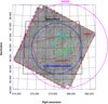 |
Fig. 1. Primary surveys located over the NEP field are used in this study. In the inner regions, the cyan circle and the green rectangle represent the SCUBA-2 (Geach et al. 2017) and the PACS (Pearson et al. 2019) observations respectively. The inner dark red rectangle shows the region of the Spitzer/MIPS data, which has no homogeneous borders. The big blue circle represents the area covered by AKARI, CFHT (Kim et al. 2012; Murata et al. 2013) and SUBARU (Oi et al., in prep.) observations. The red square corresponds to the area covered by the SPIRE (Herschel) observations (Pearson et al. 2017, and in prep.). The big magenta circle shows the coverage of GALEX data (Bianchi 2014). |
Overview of the observational data covering the NEP used in this work approximately ordered from long to short wavelengths.
This work uses the most recent data from ultraviolet (UV) to submillimetre wavelengths, primarily concentrating on the submillimetre observations from Herschel and SCUBA-2 described in Sect. 2.2 to create a multi-wavelength catalogue of high-z candidates (described in Sect. 3). We summarise the data used in this paper in the following sections. For all the catalogues described below, we always considered either total fluxes or magnitudes. Furthermore, where available, the consistency of the fluxes measured with different instruments (or different catalogues) in overlapping filters is confirmed, finding good agreement in all cases. This confirms the validity of the cross matches performed. In total, we considered 38 photometric bands with 30 of them being non-overlapping bands (see Table 2 for details).
2.2. Submillimetre data
The Herschel Space Observatory (Pilbratt et al. 2010) observed the entire NEP region as part of the Herschel Open Time Program, with the SPIRE instrument (OT2sserje012; PI Serjeant). The SPIRE observations cover an area (∼9 deg2) at 250 μm, 350 μm and 500 μm. The SPIRE catalogue is described in Pearson et al. (2017), and in prep., and contains 4820 sources, extracted via an iterative source extraction procedure (see Sect. 3.2) to optimise the detection of individual sources at 3σ higher than the extragalactic confusion noise limits of 5.8, 6.3 and 6.8 mJy/beam (1σ) at 250, 350 and 500 μm respectively (Nguyen et al. 2010).
Longer wavelength submillimetre data is also available through the SCUBA-2 cosmology legacy survey (Geach et al. 2017) at 850 μm using the Sub-millimetre Common-User Bolometer Array 2 (SCUBA-2) instrument, operating at the James Clerk Maxwell Telescope (JCMT). This survey covered the NEP-Deep area (see Fig. 1) area reaching a sensitivity of 2 mJy beam−1 (Geach et al. 2017). The SCUBA-2 catalogue at the NEP contains 330 sources which have at least a 3.5σ detection. In this study, we considered SCUBA-2 de-boosted fluxes, which allow for a proper subtraction of the background and make possible to obtain more precise estimates of the total fluxes (as for the other catalogues used in this paper). These two data sets will form the basis of our selection methods that will be used to select high-z sources over the NEP area.
2.3. Far infrared data
The NEP-Deep region was also observed in the same Herschel Open Time programme with the Photodetector Array Camera and Spectrometer (PACS) instrument (Poglitsch et al. 2010) at 100 μm and 160 μm. The survey area covered approximately (∼0.69 deg2) closely overlapping the region of the sky covered with SCUBA-2 (see Fig. 1). The PACS source extraction and catalogue is presented in Pearson et al. (2019) and contains 1385 and 630 sources to limiting fluxes of 4 and 8 mJy at 100 μm and 160 μm respectively (see Table 1). The addition of the PACS data into our data set is important to better constrain the far-infrared (FIR) spectral peak.
2.4. Mid- and near-infrared data
The NEP field has been extensively observed by the AKARI satellite (Murakami et al. 2007) as an AKARI legacy field (Matsuhara et al. 2006). The NEP was in the continuous viewing zone of AKARI and was visible several times per day allowing deep near-to mid-IR imaging of the region. The NEP was observed in all nine bands of the AKARI IRC instrument (Onaka et al. 2007): N2 (2.4 μm), N3 (3.2 μm), N4 (4.1 μm), S7 (7.0 μm), S9W (9.0 μm), S11 (11 μm), L15 (15.0 μm), L18W (18.0 μm), L24 (24 μm). Dedicated surveys were made over both the NEP-Deep and NEP-WIDE regions. The NEP-Deep catalogue of Murata et al. (2013) includes 11 349 sources over 0.5 deg2 with at least a detection in one of the AKARI bands. The use of a high S/N cut (5σ) allows for a low false detection rate (< 0.3%). The NEP-Wide catalogue (Kim et al. 2012) contains 114 974 infrared sources over a larger area of (5.4 deg2) but to a shallower depth than that of the Murata et al. (2013) NEP-Deep catalogue (see Table 1 for comparison).
Spitzer-MIPS data at 24 μm over a limited area of the NEP region is available through the Herschel Extragalactic Legacy Project (HELP)1, an ongoing program aiming to produce a multi-wavelength database sets for all Herschel extragalactic surveys (Shirley et al. 2019). HELP uses the XID+ (Hurley et al. 2017) algorithm, a deblending prior-based source extraction tool to perform photometry at the positions of known sources in far-infrared confusion dominated maps from shorter wavelength (MIPS 24 μm). The algorithm based on a probabilistic Bayesian framework which allows for the inclusion of prior information (beyond source positions and fluxes) to obtain the full posterior probability distribution on flux estimates rather than just the maximum likelihood. The availability of data with a higher spatial resolution at shorter wavelengths (optical, radio and mid-near-infra-red) enables the de-blending of Herschel maps. We note that, although SPIRE data is also included in the HELP catalogue, the photometric errors in the SPIRE band are large (the relative error is near 40% on average in the SPIRE bands). Moreover, the NEP region the MIPS observations cover about ∼2 deg2 for a total of 20 mosaics, which represent approximately a quarter of the area covered by SPIRE in the NEP field. However, the HELP catalogue is extremely valuable and we exploit this catalogue to check the reliability of the techniques that we used to cross-match all the multi-wavelength observations (see Sect. 3.2).
Observations of the NEP region at near-infrared wavelengths were also made by Spitzer during its warm mission phase with the IRAC instrument. The survey of Nayyeri et al. (2018) cover an area of a total area of 7.04 deg2, at 3.6 μm (IRAC1) and 4.5 μm (IRAC2). The final catalogue contains 380 858 sources (Nayyeri et al. 2018). The band-pass of the IRAC1 and IRAC2 filters is similar to that of the AKARI N3 and N4 filters respectively. However, the observations in the Spitzer-IRAC bands are deeper (1.29 and 0.79 μJy than the corresponding AKARI bands (∼13 μJy for N3 and N4). The deeper IRAC observations allow us to obtain additional information avoiding mismatches in our high-z multi-wavelength catalogue (see Sect. 5). The IRAC catalogue of Nayyeri et al. (2018) includes aperture photometry considering three different apertures: automatic aperture (“AUTO”), 4 arcsec (“Aperture 1”), 6 arcsec (“Aperture 2”). The fluxes computed inside these three apertures were compared to those reported for AKARI N3 and N4 in the catalogues (Murata et al. 2013; Kim et al. 2012). As a result of this comparison, we obtained the best agreement when considering the automatic apertures in Nayyeri et al. (2018), while an offset is measured for all the fixed apertures. For these reasons in this study, only the automatic aperture was considered (see our high-z DSFGs cross-matched catalogue Sect. 3.2).
2.5. Optical data
Optical follow-up surveys have been made over both the NEP-Deep and NEP-Wide survey areas. The AKARI catalogue of Murata et al. (2013) accurate cross-matching of the IR detections with their optical counterparts using B, V, R, i, z, NB711 from SUBARU-SuprimeCam, u, g, r, i, z from MegaCam-CFHT and Y, J, Ks from WIRCAM-CFHT data (see Murata et al. 2013 for details). The NEP-Wide catalogue of Kim et al. (2012), besides of the IR data, includes over ∼ 110,000 crossed-matched sources with u, g, r, i, and z band data from MegaCam-CFHT observations to a detection limit down to 26 mag (4σ) covering ∼2 deg2 of the central part of the NEP.
Additional optical data from Hyper Suprime camera (HSC) on the SUBARU telescope (Oi et al., in prep.) were also included in our multi-wavelength dataset. This data cover ∼6 deg2 in the g, r, i, z, Y optical and near-IR bands. The final catalogue contains over two million sources with a 5σ limiting magnitudes of 27.18, 26.71, 26.10, 25.26, and 24.78 mag [AB] in the five bands respectively (Goto et al. 2019). The catalogue includes 89 178 AKARI-IRC infrared sources that are already cross-matched with the observations in the optical bands.
In total, there is a broad coverage across the optical and near-mid-IR part of the spectrum, covering 28 bands in the NEP-Deep field and 14 in the NEP-Wide field. The main characteristics of these catalogues are summarised in Table 1.
2.6. Ultraviolet data
In the UV spectral range, the NEP field is covered by the Galaxy Evolution Explorer (GALEX) space telescope (Martin et al. 2005), at both far-ultraviolet (FUV) and near-ultraviolet (NUV), and contains 36 263 sources as a part of the all-sky survey described in Bianchi (2014). The observations are relatively shallow with a depth of 23 magnitude; consequently, a relatively low number of matches are expected, since most of our sources would be too faint to be detected by GALEX (see Sect. 3.2 for more details).
2.7. Spectroscopic redshift catalogues
Very limited spectroscopic data is available in the NEP region, mostly located in the NEP-Deep survey area. Some of this data were collected in the HELP catalogue of Shirley et al. (2019) and is summarised in Shim et al. (2013). The quality of the redshifts in the HELP catalogues is defined by a flag assuming a value ranging from 1 (unreliable) to 5 (high quality). There are ∼1100 sources with spectroscopic redshifts in the NEP region, however, the quality of these spectroscopic redshifts are all flagged as ≤3.
In addition to the HELP spectroscopic sub-sample, we considered the catalogue of Kim et al. (in prep.). However, the majority (84%) of the sources reported in this catalogue are located at z < 1.
We concluded that the number of sources with an available reliable spectroscopic measurement is not sufficient to complete a robust statistical analysis. For this reason, in this study we relied on the photometric redshifts (see Sect. 5.1).
3. Selection of high-z candidates and multi-wavelength catalogue
3.1. Selection of high-z candidates
In this work, the analysis focuses on two samples of high-z galaxies selected using different methods. In the first sample, high-z candidates were selected using SPIRE colour criteria, while in another case, the selection was based on SCUBA-2 fluxes.
The peak of the far-IR emission due to dust, approximately located at rest-frame λ ∼ 100 μm, can be used as a rough redshift indicator. To this purpose, observed Herschel colours are used to select potential high-z sources as these colours allow sampling of the peak of the dust emission at different redshifts. Submillimetre-FIR colour-colour diagrams are commonly used to find high-z candidates (e.g. Amblard et al. 2010; Ivison 2012). A similar concept is utilised by the 500 μm risers method, where sources exhibiting increasing SPIRE fluxes moving from 250 μm to 350 μm and then onwards to 500 μm are more likely to be located at very high redshift, since the dust emission peak appears to be redshifted to λ > 500μm (z > 4). The 500 μm riser criterion is successful in selecting massive high-z sources (Donevski et al. 2018). The use of submillimetre colours to select high-z candidates relies on the redshifting of the source SED through the observation bands, defining the colour-colour parameter space where potential high-z sources will lie (see Fig. 2). We therefore define a SPIRE colour criteria following Amblard et al. (2010) of F350 μm > 35 mJy and F500 μm/F250 μm> 0.75 in order to select a total of 268 high-z candidates from our SPIRE catalogue, these sources are expected to lie at z > 2. In addition, the 500 μm riser colour (F500 μm > F350 μm > F250 μm) criterion was applied to select 41 high-z candidates, 23 of which not already included in the high-z sample.
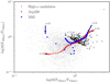 |
Fig. 2. Colour–colour diagram of the SPIRE fluxes with the tracks of the local starburst galaxies M82 (blue) and Arp220 (red) over-plotted. The tracks represent the observed colours as expected from the same SEDs observed at different redshifts from z = 0 to z = 6 with redshift steps of Δz = 0.1 The bold points are the high-z candidates which lie in the same colour space than the evolved tracks at z > 2. The upper right area of the plot shows the average error bar for the high-z candidates. all these methods are based on MBB models, where the redshift evolution of the SEDs is not included. Therefore, more sophisticated SED templates should be used to investigate the correlation between redshift and colours. |
The previous criteria are based on modified black body models. We added another criterion where the redshift evolution of the SED taken intro account (Yuan et al. 2015). We find 102 new sources that follow the colours F500 μm/F350 μm > 1.1 ⋅ (F250 μm/F350 μm)−0.15 (Yuan et al. 2015). This use of several colour criteria allow us to obtain a high-z sample, not only with extreme sources at z > 4 (e.g. Asboth et al. 2016), to study the properties of DSFGs and their evolution over redshift (see Sect. 5).
Our second high-z sample is constructed independently by applying a threshold to the SCUBA-2 fluxes. In particular, we selected only sources characterised by F850 μm > 3 mJy, from the catalogue of Geach et al. (2017). In total, 422 sources comply with this criterion which is most likely to select sources at z ∼ 2 and less massive than those selected using the SPIRE colours (Casey et al. 2014).
Using these two criteria; SPIRE colours and SCUBA-2 flux, we selected a total of 291 high-z candidates using SPIRE colour criteria (268 with Amblard criteria, 23 risers and 140 with Yuan criteria) and 422 sources using the threshold applied to SCUBA-2 fluxes. We refer them as SPIRE selected sources, and SCUBA-2 selected sources, respectively. We noticed and expected that the number of potential high-z sources is significantly reduced when we cross-matched the submillimetre detections with the rest of the multi-wavelength data after checking the fitted SEDs for possible mismatches (see Sects. 3.2 and 4, respectively).
3.2. Multi-wavelength high-z catalogue
The high-z candidates selected were cross-matched with the data available in the NEP region (see Sect. 2) associating every detection in each band to the closest counterpart in the others. The SPIRE maps suffer from lower resolution and photometric confusion leading to the blending of multiples sources due to the relatively large beam areas of Herschel-SPIRE, ranging from 17.6–35.2 arcsec from 250–500 μm respectively (Griffin et al. 2013). To minimise these effects and to aid in our multi-wavelength cross-matching, the SPIRE catalogue of Pearson et al. (in prep.) was created via an iterative extraction procedure to optimise the detection of individual sources. A similar approach has been used to successfully extract sources for the Herschel HeViCS programme (Davies et al. 2010; Pappalardo et al. 2015), identifying bright peaks in the maps and then fitting with the SPIRE 250 μm PSF. In an iterative process, the most luminous sources extracted are subtracted from the original image, then, the source extraction is performed on this new cleaned image, but this time considering a lower detection threshold. The iteration is repeated until the extraction threshold reaches the level of the noise. Photometry at 350 and 500 μm is obtained considering the 250 μm prior positions. Similar approaches have been adopted in other other large-area surveys with Herschel (e.g. Clements et al. 2010; Rigby et al. 2011).
As stated above, the catalogues are matched by pairing the closest counterparts in different photometric bands. To this purpose, when matching two bands, we considered a search radius corresponding to 0.5 * FWHM of the band with the larger PSF. A similar technique is successfully adopted in Baronchelli et al. (2016, 2018).
3.2.1. SPIRE colour selected sample
The multi-wavelength catalogue for the high-z DSFGs selected via SPIRE colours was made using the 250 μm SPIRE position (the highest resolution band) and their closest longest wavelength band counterparts. Counterparts in the SCUBA-2 catalogue of Geach et al. (2017) were cross-matched with the 250 μm band using a search radius smaller than nine arc-seconds, (half of the SPIRE beam FWHM at 250 μm). Most of the SPIRE selected high-z candidates (74%) have an 850 μm counterpart following the classical definition of a SMG (F850 > 3 μmJy).
PACS data was incorporated by producing the photometry in the PACS maps at the SPIRE 250 μm position of the high-z candidate. The photometry was produced using an identical procedure to that of Pearson et al. 2019 in both PACS maps at 100 μm and 160 μm. In this way, a PACS flux (or at least an upper limit) can be recovered for all our high-z candidates. As a means of validation of our PACS photometry, we compared the brighter PACS fluxes to confirm that they have the same measured flux as by cross-matching SPIRE candidates directly with the PACS catalogue of Pearson et al. (2019). The addition of PACS photometry produces complete coverage of the FIR peak for the sources located in the deep field.
Infrared counterparts in the NEP-Deep Murata et al. (2013) and NEP-Wide Kim et al. (2012) catalogues (including their optical counterparts in the catalogues) were cross-matched with the high-z catalogue using a search radius is 9 arcseconds (half of the SPIRE 250 μm beam) considering the possible counterparts inside this search radius. For both catalogues, in order to select the correct counterpart, the longest wavelength mid-infrared 15 μm and 18 μm bands were used.
For the optical Subaru-HSC data, which covers both deep and Wide field, the mid-infrared bands are used effectively as an “IR-bridge” (Baronchelli et al. 2016), choosing the optical detection associated with the brighter IR detection. The two AKARI catalogues and optical data overlapped, the associations were compared band by band, finding a good agreement of fluxes between them.
The Spitzer-IRAC catalogue with 3.6 and 4.5 μm bands (Nayyeri et al. 2018) was cross-matched using a search radius of 9 arcseconds with the 250 μm SPIRE band, finding 261 identifications in at least one of the IRAC bands. We note the same percentage of matches in the deep than in the wide field (80%) although the SPIRE data is deeper in the NEP-Deep region. These sources were analysed with CIGALE in Sect. 4. However, only the high-z candidates with more data than SPIRE and IRAC detection were included in Sect. 5. Where sources had flux detections in both the AKARI-IRAC and AKARI-IRC overlapping bands, the source fluxes were verified to ensure that the same source was associated in both cases.
As an additional level of validation, the HELP catalogue was also used to check any miss-associations between IRAC and SPIRE data, since the HELP catalogue contains SPIRE sources. The HELP catalogue was cross-matched with our high-z catalogue based on the 250 μm positions using a 3 arcsec search radius. We find that the associations between the two SPIRE catalogues agree in flux, within the errors (see Appendix A and Fig. A.1) and we find extremely few sources with double counterparts. This flux agreement not only shows that we are selecting the same sources but also emphasises that the source identification and the extraction method used in Pearson et al., in prep, which covers four times more area than in the HELP catalogue (see Table 1) successfully deblends the SPIRE sources. The HELP catalogue also includes Spitzer 24 μm data and as a result of this cross-match, ten identifications at 24 μm were incorporated into our multi-wavelength catalogue.
Finally, the UV GALEX catalogue was cross-matched with the optical counterparts with a search radius smaller than 4 arcseconds (half of the beam radius). However, only 13 sources of the final sample have a UV counterpart, due to the shallow coverage of GALEX.
Summarising, the final high-z DSFG catalogue contains 25 high-z candidates with coverage over 38 photometric bands approximately defined over the NEP-Deep area and 266 high-z candidates with coverage over 26 bands in NEP-WIDE area. In total, our high-z DSFG catalogue contains 291 (266+25) sources.
The SPIRE and the AKARI-IRC catalogues are deeper in the NEP-Deep region and, due to the differences in both the number of photometric bands and depth, the analysis in Sect. 5 was produced separately for the Deep and the Wide fields.
3.2.2. SCUBA-2 selected sources
The 288 SCUBA-2 selected galaxies were cross-matched with the rest of the data described in Sect. 2 using the original SCUBA-2 positions as the reference. The SPIRE catalogue was cross-matched by using a nine arc-second search radius. In total, three double detections between the SPIRE and SCUBA-2 catalogues were found. In these cases, the closest counterpart was selected. For the SCUBA-2 sources with no cross-match in the SPIRE catalogue, the photometry was calculated using the SCUBA-2 position in each of the SPIRE maps, in the case of no detection, the upper limits for the 3 SPIRE bands were incorporated.
The PACS data, at 100 and 160 μm, were included by cross-matching with the SCUBA-2 positions using a 7.5 arcsec search radius finding identifications for 13% of the sources.
The SCUBA-2 survey lies within the Spitzer-MIPS 24 μm coverage (see Fig. 1), and all 288 SCUBA-2 sources were cross-matched with 24 μm HELP catalogue using a 7.5 arcsec. search radius (half of the SCUBA-2 beam size). We find 123 SCUBA sources with a reliable detection, the rest (165 high-z candidates) were not included in the analysis since they have either an unreliable 24 μm flux or a lack of counterpart. Using the 24 μm source position, these data were taken as an “IR-bridge” (Baronchelli et al. 2016) for incorporating the ancillary data at shorter wavelengths. The AKARI infrared and associated optical CFHT and SUBARU data (SuprimeCam) from Murata et al. (2013) over the NEP-Deep region were incorporated with a 3 arcsec. search radius. The deeper SUBARU-HSC data (Oi et al., in prep.) were incorporated by using with the same search radius. Where the optical bands overlapped in two or more of the Murata et al. (2013) AKARI, SUBARU-HSC, HELP catalogues the positions and photometry were found to be in good agreement, reinforcing our cross-matching confidence.
The final sample of SCUBA-2 sources (SMGs) contains 123 sources, covering 37 photometric bands, similar to the DSFGs selected via the SPIRE colours in the NEP-Deep field. Therefore, the results of the two samples can be compared to further decrease possible instances of a miss-match and removing less reliable associations from the final sample (see Sect. 5).
4. Methodology: SED fitting with CIGALE
The physical properties of our high-z sample were calculated using SED fitting techniques with the CIGALE software (Code Investigating GALaxy Emission, Burgarella et al. 2005; Noll et al. 2009; Boquien et al. 20192). CIGALE is a SED fitting code based on the physical properties of galaxies that covers the spectrum from UV to radio wavelengths, taking into account the balance between the energy emitted in the UV-optical, absorption by dust, and the reprocessing of the starlight into the IR. In this section, we describe the modules tested within CIGALE. Table 2 describes the main parameters of each module that was finally selected.
Main modules and input parameters used in CIGALE for the analysis of the high-z sample.
As the first step, CIGALE builds a stellar component defining the energy emitted by stars. This stellar component takes as an input an assumed star formation history (SFH) defined in an independent module in CIGALE, which is crucial in estimating the SFR. Several SFHs describing the star formation of galaxies across cosmic time are available considering different physical processes depending on the nature of the galaxy. DSFGs tend to have high star formation, and the possibility of having a burst of star formation was evaluated by using a double decreasing exponential SFH defined as:
 (1)
(1)
where tburst is the age of a second episode of star formation in the galaxy and tmain corresponds to the age of the main population of the galaxy. This SFH assumes a decreasing exponential with a presence of a starburst if the fraction of the burst fburst > 0 or only a decreasing exponential if there is no starburst (see Fig. 3), where τmain and τburst are the e-folding times of the main and burst populations respectively.
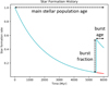 |
Fig. 3. Star formation history (SFH) adopted in this work: a double-exponential decreasing with starburst age. A decreasing exponential describes the star formation with the age of the main stellar population of the galaxy (tage) plus a burst of star formation at a specific epoch (tburst) with a burst fraction (fburst) defining the intensity of the burst. |
The exponential SFH provides the best estimates of Mstar and SFR, but the ages may not be as realistic as with other SFH (Ciesla et al. 2015). We applied a broad range of values in this model to allow the possibility of either a moderate or an intense burst of star formation. Besides, the broad range of ages allows different redshifts.
After computing the SFH, a single stellar population library is needed for modelling the stellar spectrum. The widely used Bruzual & Charlot (2003) model assumes a single stellar population by isochrone synthesis, which takes stars of the same age and integrates their spectra to compute the total flux. The disadvantage is that the isochrones are calculated in discrete steps in time and therefore, any stellar evolution more rapid than these time steps is not well represented. For this reason, we compared the alternative Maraston (2005) models, which are fuel-consumption based algorithms that follow a “turn off” from the main sequence of stars. In both stellar population models, we assume the initial mass function given by Chabrier (2003) and a solar metallicity Z⊙ (see Table 2) as a standard assumption that allow us to compare our results with the rest of the literature.
The nebular emission module, based on the empirical templates of Inoue (2011), describes the spectral (line) emission, which is essential in star-forming regions and high-z redshift galaxies (Stark et al. 2013). This emission has a direct impact on the SED modelling, and it can increase the average flux by up to 10% in the case of the most energetic spectral lines (Noll et al. 2009). We find that SFR is lower when the nebular emission is considered, since a fraction of the radiation contributes as nebular emission instead of the continuum emission of the galaxy.
For the dust attenuation, three different options were investigated. The most common attenuation law for star-forming galaxies is the Calzetti et al. (2000) law with an extension to shorter wavelengths in the spectrum provided by Leitherer et al. (2002). The second model, proposes a simpler attenuation power-law (Charlot & Fall 2000), that assumes that all the stars are attenuated by diffuse dust in the same manner. However, a single attenuation curve proves to be insufficient to describe DSFGs, particularly at high-z (Noll et al. 2009) and it is not appropriate for our sample. The third model described in Boquien et al. (2019) extends the model of Charlot & Fall (2000) and combines both the birth cloud attenuation and the interstellar medium attenuation each represented by a power law, and therefore makes a distinction between the young and old stellar emission. This has been shown to characterise well the emission from ULIRGS at z ∼ 2 (Lo Faro et al. 2017).
CIGALE was tested with all three dust attenuation options. Although we did not find any significant differences in the goodness of the fits between these models, the third option was selected on the basis that it makes a distinction between the stellar emission components which is more appropriate for IR galaxies (Buat et al. 2018; Małek et al. 2018). The main parameters that define the model are the attenuation (AV) and the slopes of the 2-power law attenuation for the birth cloud and the interstellar medium (see Table 2).
Models for the emission at mid-infrared (MIR) wavelengths are complex since they require the addition of PAH emission (dust features which are extremely grain size dependent). Our sample of dusty high-z galaxies was tested with both the Draine et al. (2014) and Schreiber et al. (2016) models. Draine et al. (2014) takes into account the emission from small dust grains and the characteristics of intense MIR emission (extreme heating environments tend to stop the process of dust formation) typically present in star-forming galaxies. The model is carefully described in Draine & Li (2007) with and the updated version that allows higher dust temperatures (Draine et al. 2014). The main parameters are the mass fraction of the PAH population (qpah) and the minimum radiation field (Umin) which is related to the dust temperature (Aniano et al. 2012). We set big Umin values to allow higher temperatures (see Table 2). The Schreiber et al. (2016) model is a simpler alternative with regards to the PAH emission, being instead more focused on the FIR-submillimetre peak. We used the bayesian interference factor (BIC) to compare the goodness of the fit of two models. The difference between Schreiber et al. (2016), and Draine et al. (2014) is △BIC ∼ 6 in the advantage of Draine et al. (2014) meaning that is significantly better (Ciesla et al. 2018). In addition, the models of Casey (2012), also commonly used for fitting DSFGs, were investigated. However, this model mainly considers the long-wavelength fitting to a modified black body with dust temperatures of ∼35 K. It does not take into account the near and mid-IR data, excluding the PAH contribution. Hence these two models, Casey (2012) and Schreiber et al. (2016), were tested but not used in the results.
The presence of an AGN can break the balance between the absorption and emission from dust, due to their characteristic non-thermal emission. Fritz et al. (2006) provides the primary model for the AGN contribution in CIGALE. In terms of the SED fitting, the AGN contribution is mainly an additional mid-infrared dust component. Fritz et al. (2006) accurately takes into account the AGN modelling, described by parameters such as the radii and opening angle of the dust torus, and the angle between the AGN axis and line of sight. The model is provides the AGN fraction (0 < fAGN < 1 where 1 is the 100%). In this work, we used the AGN model for a broad classification of AGN presence or non-presence in the galaxy. However, the optical depth and the opening angle give the option of a Type 1 AGN (unobscured), Type 2 (obscured), an intermediate template or non-AGN (see Table 2). The rest of the values were set to the typical values (Fritz et al. 2006) in order to avoid degenerate model templates.
The combination of the modules described above, with the grid of selected primary parameters in Table 2, produces ∼465 million potential spectral templates for each source. CIGALE takes into account those templates and computes the SED fits, selecting the best probabilistic result by a Bayesian approach (see Noll et al. 2009 for details). The best fit SED and probability distribution function (PDF) (see example in Fig. 4 left and right respectively) of each of our high-z candidates were visualised individually to remove sources with a possible miss-match, gravitational lenses or an energy balance problem (see Sect. 5).
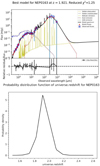 |
Fig. 4. Left panel: example galaxy SED fit from our sample produced by CIGALE with the modules taken into account in the legend. The blue squares are the observed fluxes in mJy, the red dots represent the corresponding predicted fluxes by CIGALE that lie on the black line model fit. Bruzual & Charlot (2003) reproduces the stellar component, where the orange line is the stellar attenuation whereas the blue line shows the unattenuated stellar emission. The green line is the AGN component, modelled by the Fritz et al. (2006) (no green line implies no AGN presence). The dust component is represented by the red line (Draine et al. 2014). The emission lines are shown in pale yellow. The upper part of the plot shows the ID of the source, the redshift and the reduced χ2 fit result. Right panel: corresponding probability distribution function (PDF) of the estimated photometric redshift for the source in the left panel. The PDF peaks at redshift zphot = 1.9. CIGALE produces a Bayesian analysis for each parameter selecting the most likely result. |
An additional quality check is provided by the CIGALE software in the form of a set of estimated flux densities. CIGALE produces a mock catalogue of photometry where the flux densities are known from the best fit model. This mock photometry can also be used to calculate the exact physical parameters which can then be compared with the estimated values (see Boquien et al. 2019 for details). The reliability of the photometric redshift was validated together with the rest of the physical parameters comparing the real value with the estimated value for each source (see Fig. 5).
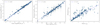 |
Fig. 5. Quality analysis was produced with the mock photometry to calculate exact values for selected physical parameters: the star formation rate, the stellar mass and the photometric redshift. The x-axis represents the exact parameter calculated from the mock photometry from the best fit, the y-axis represents the estimated value presented in the results. The blue line is the regression line with the correlation coefficient shown in the top-left of each panel. The good agreement between the two values implies a good reproducibility for the SFR, stellar masses and photometric redshifts. |
5. Results
The SED fitting using CIGALE was performed on our high-z sample (Sect. 4), in order to calculate the physical parameters such as the stellar and gas masses, star formation rates and photometric redshifts. Sources with less than seven photometric detections were not included in the following statistical analysis, due to the limitation in calculating reliable stellar masses and SFRs. However, this lack of photometric data in the optical-NIR wavebands could also be indicative of their high-z nature, so we do not disregard them out of context. The part of these sources with photometric redshifts, z > 3 (51 sources, most of them with only SPIRE and IRAC data) are listed in Appendix A. In addition, after visually checking the fitted SED, sources that were either probable miss-matches or possible gravitational lens candidates were also removed from the statistical sample (Małek et al. 2018).
We distinguish between the NEP-Wide and NEP-Deep areas during the analysis due to the difference in the number of bands and depth of the AKARI and SPIRE data. In the NEP-Deep field, 88% of the galaxies have more than twelve photometric detections, and on average detections in more than ∼20 bands. In the NEP-Wide field, the number of sources with more than ten photometric detections is 60% with on average detection in 11 photometric bands.
The final sub-sample with good multi-wavelength coverage and discarding mis-matches contains 185 high-z dusty galaxies: 78 in the NEP-Deep field and 107 in the NEP-Wide field.
5.1. Photometric redshift
Photometric redshifts are often used as a proxy in large surveys due to the lack of available spectroscopic redshifts which are observational time-consuming to collect. In particular for DSFGs, the high amounts of dust present at high redshift makes redshifts from optical lines impossible to obtain, and the use of photometric redshift is the only viable route for large sample of galaxies (see e.g. da Cunha et al. 2015).
We used CIGALE to calculate the photometric redshift for the final selection of 185 high-z galaxies with good photometric coverage. The photometric redshift – and consequently, the rest of the physical parameters, depend on the models assumed in CIGALE. CIGALE takes into account the entire spectral range to calculate the photometric redshift. Hence, the selection of the dust emission model can produce differences in the photometric redshifts.
The average redshift for the entire high-z DSFG sample, independent of the selection method (SPIRE colours and SCUBA-2 flux, was found to be z = 2.33 ± 0.08 (0.1 < zphot < 5.6). The redshifts for the sources selected with SCUBA-2 fluxes is on average lower than the sources selected via SPIRE colours. The latter sample peaks at a higher average redshift with median  , whereas the SMGs have a median redshift of
  . The redshift distribution of the two populations is shown in Fig. 6. The redshift distribution over the NEP-Wide and NEP-Deep fields were found to be similar and are represented together in the histogram in Fig. 6. The higher redshift nature of the SPIRE selected DSFGs indicates that the 500 μm riser method and SPIRE colour-colour diagrams select on average higher redshift sources than with SCUBA-2 fluxes, as expected. There was not found to be any dependence of the photometric redshift on the number of photometric bands.
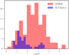 |
Fig. 6. Histogram of the calculated photometric redshifts for the two selection methods: sample selected with SCUBA-2 fluxes (blue) and selected with SPIRE colours (red). The sample selected via SPIRE colours peaks at a higher redshift with a median value of |


We also investigated the spectroscopic data sets available over the NEP field (Shim et al. 2013, Kim et al., in prep., see Sect. 2.7). Unfortunately, spectroscopic data is only available for 10 of our sources in our high-z catalogue (4 for the SCUBA-2 selected galaxies and 6 for the SPIRE selected galaxies, that is < 5% of the sample). This is not a large enough sample to extract any conclusions on the quality of the photometric redshift estimate. For the handful of spectroscopic redshifts that are available, these were obtained from optical and NIR lines and all have low-quality flags in the spectroscopic catalogues. Therefore, to confirm the quality of the photometric redshift, spectroscopic data from sub-millimetre telescopes is proposed for future work (see Sect. 7).
Using the photometric redshift, CIGALE calculates the infrared luminosity. Figure 7 shows the resulting luminosity-redshift distribution for each of our selection criteria. The SPIRE selected sources are further split into sources in the NEP-Deep and Wide fields. The calculated luminosity in the NEP-Wide and NEP-Deep field is similar over the same redshift range, and is therefore not biased by the depth of the data. From Fig. 7, it can be seen that almost all of the sources are ULIRGs, as expected, and with z < 1 are mostly sources selected with SCUBA-2 flux method. The detection limit reached for SPIRE at the shortest wavelength is ∼10 mJy whereas for the SCUBA-2 is ∼3 mJy.
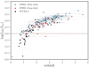 |
Fig. 7. Infrared luminosity (LIR) against photometric redshift for the NEP-Deep field (black and red dots) and the Wide field (blue dots), with the selection method detailed in the legend. The red dashed line shows the limit for ULIRGs LIR > 1012 L⊙: above which the sources are either ULIRGs (50%) or hyperluminous infrared galaxies (HLIRGs; LIR > 1013 L⊙) (36%). The remaining sources below the line (14%) are classified as luminous infrared galaxies (LIRGs, 1011 L⊙ < LIR < 1012 L⊙) The galaxies selected with the SCUBA-2 method have the same number of photometric bands as the sources selected with SPIRE in the NEP-Deep field, however, the SPIRE colour criteria select, on average, more luminous sources (15 % more) than galaxies selected with SCUBA-2. |
Due to the larger areal coverage, there are four times more luminous galaxies at z > 3.5 in the NEP-Wide than in the NEP-Deep field. However, the galaxies selected with the SCUBA-2 method are 15 % less luminous on average than the galaxies selected via the SPIRE colours over the same area with the same number of bands. It appears that SPIRE colour and 500 μm techniques tend to select more luminous galaxies, probably because they are more massive and warmer (see Sect. 5.2).
A total of 12 sources are detected at z ≳ 4 from both selection methods combined. This number can be compared with the surface density predicted by the contemporary galaxy evolution models of Pearson et al. (2017). Over a similar area, Pearson et al. (2017) predicts around 20 sources above the SPIRE confusion limit at z > 4. Taking into account the fact that some of our high-z sources were rejected due to the low number of photometric detections (10 of the rejected list have z ≳ 4, see Table B.1), the predictions are broadly consistent with the numbers presented here.
5.2. The star formation rate and the main sequence of galaxies
The star formation rate (SFR) and the stellar mass were computed to determine the position of our high-z sources on the main sequence (MS) of galaxies, to address whether DSFGs selected at sub-millimetre wavelengths lie on the MS or above it as outlying starbursts.
The median star formation rate for the entire sample of 185 DSFGs is 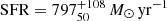 . Over the NEP-Deep field we see a clear distinction between sources selected using SCUBA-2 flux (
 ) and SPIRE colour (
 ) criteria. The SCUBA-2 flux method is able to select relatively faint sources with a more moderate star formation rate than the extreme sources detected with SPIRE colours (see e.g. Riechers et al. 2013; Rowan-Robinson et al. 2016, 2018). The extremest source we find have SFRs < 7000 M⊙ yr−1 The median SFR over the NEP-Wide field is higher (
 ), however, both fields exhibit more moderate SFRs than reported in previous work (e.g. Rowan-Robinson et al. 2016, see Sect. 6 for discussion).
We calculated the stellar mass for our sample using CIGALE. Two different stellar population models were tested and the SED fitting was run for both the Bruzual & Charlot (2003) and Maraston (2005) models supported by CIGALE. No significant differences in the results were found that would change the position of the sample relative to the MS of galaxies.
We conclude that the enormous differences in submillimetre galaxies discussed in the literature (see e.g. da Cunha et al. 2015; Dunlop et al. 2017) are not influenced by using stellar populations models based on isochrones such as Bruzual & Charlot (2003) instead of turn-off based models such as Maraston (2005). For this work, the models of Bruzual & Charlot (2003) were finally chosen in order for us to compare our results with the work in the literature that uses the alternative MAGPHYS SED fitting code, which uses the same population model (e.g. da Cunha et al. 2015; Miettinen et al. 2017).
The main sequence of galaxies is known to evolve with redshift and for this work, the definition of Speagle et al. (2014) was applied to
 (2)
(2)
where tz is the age of the Universe in [Gyr]. Note that the definition is function of redshift and we considered the MS at the corresponding redshift for each galaxy. A galaxy is commonly considered “above the MS” if its position is a multiple of times above the definition of the MS line. The correlation is not strictly a line and has some scatter which makes considere galaxies above the MS if their SFR is several times above the line. da Cunha et al. (2015) uses a criteria of three times above the MS, although others assume different criteria, such as Elbaz et al. (2011), who defines the MS as a function of cosmic time and considers the sources two times above the MS as outlying starburst galaxies. Here, in order to compare our results with da Cunha et al. (2015) and Dunlop et al. (2017), who assume the same definition of the MS as Speagle et al. (2014), all sources that are three times above the line of the MS are considered to be above the MS and therefore to be starburst galaxies (see Fig. 9).
We find that 38% of our sources would be defined as starbursts lying three times above the MS. The remaining sources being on the MS despite of their high SFRs because they are massive galaxies, which can be visualised by computing the specific star formation rate sSFR = SFR/Mstar (see top-panel of Fig. 8). The bottom-panel of Fig. 8 shows the number-redshift distribution of the starburst and main sequence galaxies. Most starburst galaxies are found at z = 2−4 with activity descreasing to higher redshift z > 4 (however, this decrease is accompanied by a decrease in the sample that makes difficult to be certain of evolution of the starburst activity with redshift).
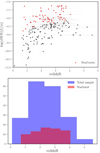 |
Fig. 8. Top panel: specific star-formation rate (sSFR) against redshift for the total sample. The galaxies classified as starbursts using the definition of Speagle et al. (2014) are marked as red dots and are seen to exhibit a higher sSFR than the rest of the population. Bottom panel: number-redshift distribution of the total sample (blue bars) and the starbursts (red bars). The fraction of starbursts increases up to z = 2, and it is similar out to z ∼ 3−4 (around 40%), decreasing to higher redshifts z > 4. A larger sample at z > 4 would be required to investigate the evolution of the starbursts over cosmic time. |
In order to evaluate their position in the MS and any evolution with cosmic time, the sample was segregated into four redshift bins (1.5 ≤ z < 2.5, 2.5 ≤ z < 3.5, 3.5 ≤ z < 4.5 and 4.5 ≤ z < 5.7). Figure 9 shows the main sequence for the redshift bins centred on the redshifts z = 2 and z = 3 respectively. The fraction of starburst galaxies is highest in the z = 2 redshift bin (43%), decreasing slightly to z = 3 (40%) over a similar size sample. The rest of the redshift bins are too sparsely populated to draw robust conclusions on any evolution of the MS with redshift in our sample and are not shown in the figure. We further compared the position on the MS for our two selection methods, over the NEP-Deep field, where there are the same number of bands, and similar depth. We find 12 % more galaxies classified as starbursts using the SPIRE colours compared to the SCUBA-2 selected sources.
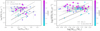 |
Fig. 9. Main sequence of galaxies. The black line shows the MS as defined in Speagle et al. (2014), with the dashed lines showing three times above and below the line of the MS for this redshift bin. The sources considered as starburst are three times above the MS. Left panel: main sequence of galaxies for the redshift bin at 1.5 ≤ z < 2.5. In the z = 2 bin the fraction of starbursts with respect to the number of sources is 43%. Right panel: main sequence of galaxies for the redshift bin at 2.5 ≤ z < 3.5. In the z = 3 bin the fraction of starbursts with respect to the number of sources is 40%. In both cases the starbursts tend to be of lower stellar mass than the majority of sources lying on the MS. |
5.3. The effect of AGN
We also investigated the effect of any AGN presence and associated PAH deficit (Elbaz et al. 2011), both significant parameters that could affect the star formation rate, thus influencing the positions of sources on or off the MS. The photometric bands allowing to probe the PAHs contribution and AGN presence in mid-IR are the AKARI bands (S9, S11, L15, L18, L24), and the Spitzer (MIPS1) (see Sect. 2). We use CIGALE to estimate any possible AGN contribution to a spectral fit assuming the AGN model of Fritz et al. (2006). Approximately 12% of the high-z sample have an AGN presence of more than 20%, with a handful of sources classified as AGN dominated. We do not find a correlation between AGN presence and SFR or redshift (see Fig. 10), neither with a high AGN fraction being specifically associated with the starburst galaxies above the MS. However, any AGN presence will affect the estimated SFR (of the order of < 10% for the majority of our sample) and it is necessary to take an AGN model to the study of DSFGs.
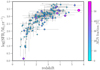 |
Fig. 10. SFR against redshift with the AGN fraction in the colour bar: 12% of the high-z sample have an AGN presence of more than 20% with no correlation with redshift. |
The contribution from PAHs concentration was evaluated using the Draine et al. (2014) dust models (see Table 2). We do not find any PAH deficit in the starburst galaxies having a similar fraction of PAHs for galaxies above or on the MS. The sources that show a high AGN presence have small or non-PAH fractions as expected due to grain destruction by the intense radiation from the AGN, especially at the highest redshifts (z > 4).
5.4. Star formation efficiency
The star formation efficiency (SFE) relates the star formation rate to the gas mass (SFE = SFR/Mgas) and is a measure of how efficiently the gas is processed into stars. The SFE allows us to analyse the factors that trigger the star formation. We compared the SFE of the populations both above and on the MS in our sample to see if there is a factor that can trigger the star formation or if it is simply the fact that they contain more gas.
The mass of the gas is calculated by applying a conversion factor for the dust-to-gas ratio, to the mass of the dust derived from the Draine et al. (2014) models. There is evidence than high-z submillimetre galaxies are dust rich, however, the high dust content is proportional to the high gas content, having a dust-to-gas ratio higher or similar to normal spiral galaxies (Santini et al. 2010).
In Fig. 11, the SFE is plotted as a function of redshift for our entire high-z sample. The SFE correlates with redshift, being the sources at higher redshift being more efficient at forming stars. Also shown in Fig. 11 (top-panel colour bar) is the age of the burst of star formation in the galaxy as derived from CIGALE (as described in Sect. 4 and Fig. 3). The age of the burst in the galaxy corresponds to the moment that the burst occurs in the time of the galaxy. We find a clear trend between the age of the starburst in the galaxy and the efficiency of the star formation: the later the burst is in the age of the galaxy, the more efficient the star formation.
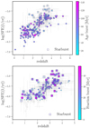 |
Fig. 11. SFE as a function of redshift. A general trend of increasing SFE with redshift is seen. SFE as a function of redshift. A general trend of increasing SFE with redshift is seen. This trend is more prominent in the starburst population (above the MS) identified by the blue border squares around the circles in the plot. Top-panel: dependence of the results on the age of the starburst (in the colour-bar). There is a clear dependence between the efficiency of star formation with the age of the starbursts: the later the starburst in the age of the galaxy the more efficient the star formation. Bottom-panel: same SFE-redshift plot with the dependence on the fraction of the star-formation burst (in the colour-bar), the more significant burst, the more efficient the star formation. |
The age can be a difficult parameter to calculate thought SED fitting modelling (Buat et al. 2014). Also, the mock test shows a bad estimation for the age of the burst with a poor linear regression (r2 = 0.3). For this reason, we also evaluate the presence of any starburst by the parameter fburst with a better result in the mock catalogue (r2 = 0.7) than the age of the burst. The starburst fraction has an effect on the SFE of the galaxy, the more massive the starburst, the bigger the triggering of star formation (see Fig. 11 bottom-panel).
We find no relation between either the AGN fraction or the PAH concentration with the SFE, which was expected from the previous lack of correlation between those parameters with the star formation discussed in Sect. 5.3.
The presence of a starburst could be due to a merger. To confirm this, the morphology of the source would be required. As future work, the SFE will be calculated by tracing the molecular gas via spectroscopic observations to study the compactness of the sample. Furthermore, the SFH parameters are challenging to constrain from broadband SED fitting and spectroscopic observations will help to better calculate these parameters (see future work in Sect. 7).
6. Discussion
There is no explicit consensus on the nature of sub-millimetre galaxies over cosmic time. In this Section, we discuss the reasons for the differences in our results with previous studies and give our vision of the nature of sub-millimetre galaxies, discussing their position on the MS, shedding some light on the considerable disagreement in the literature, explaining if the difference relies on selection effects or model considerations.
6.1. High-z selection at submillimetre wavelengths
We studied the high-z population at the NEP by using two different sub-millimetre selection criteria: SCUBA-2 selected sources at 850 μm and selection by SPIRE colours including the 500 μm riser technique. This approach allows us to evaluate if the different results in previous works could be due to a selection effect. The SCUBA-2 selected sample has a significantly lower fraction lying above the MS compared to the SPIRE colour selected sources at shorter wavelengths (see Sect. 5). The SCUBA-2 methods appear to select sources at lower IR luminosity than the SPIRE selection method over the same NEP-Deep field and, in consequence, lower star formation. Such a difference in SFR due to the different population could influence the different outcomes in literature, but it is not big enough to be the main reason for the disagreement. We find lower star formation rates than Rowan-Robinson et al. (2016) using the same selection method, which implies that these differences are not a selection effect. These extreme star-forming galaxies are “monsters” with large stellar masses and SFRs. However, both the consideration of an AGN presence and avoiding fitting with local galaxy templates (e.g. Arp220, M82, Polletta et al. 2007), it is possible to lower the estimated SFRs by an order of magnitude.
6.2. The position of high-z SMGs on the MS
We find that the position of galaxies on the MS relation cannot only be explained by selection effects. Assumptions in the modelling approach, such as the different physical models in the SED fitting, can affect the calculation of the SFR and stellar masses. We investigated the differences from assuming stellar population models by using the models of Bruzual & Charlot (2003) and Maraston (2005). Although there were small differences in the estimated SFR and stellar masses, these differences were not enough to change the position of the sub-millimetre galaxies in the MS diagram significantly.
Our results are in disagreement with some previous studies such as Ikarashi et al. (2017), where 72% of their submillimetre selected sample lie above the MS with 1.4 ≤ z < 2.5, or with Miettinen et al. (2017) who measures 63% of SMGs above the MS. Some of this discrepancy could be since we take into account the AGN contribution in the fitting, which imply lower SFRs, and the differences in the code assumptions (we use CIGALE instead of MAGPHYS). The AGN emission has an influence on the MS slope up to 32 % depending on the SFH and the type of AGN (Ciesla et al. 2015). Note that in particular, the MAGPHYS SED fitting code uses the Bruzual & Charlot (2003) models, which means that we should find similar stellar masses with CIGALE. However, SFRs may differ due to the different SFH and the lack of AGN models. Hence, with similar stellar masses and different SFRs, it will change the position in the MS.
Other submillimetre samples, such as Dunlop et al. (2017), suggest that all their sources lie on the main sequence. This disagreement with our results may indeed be a selection effect since Dunlop et al. (2017) is a deep pencil-beam survey, and it is sensitive to lower SFRs but comparable stellar masses.
Another reason related to the modelling itself is the use of local templates for galaxies to calculate photometric redshifts, which tend to give higher redshifts (Ma et al. 2019) and higher SFRs. Finally, assumed the SFH could produce a different SFR.
Consequently, it is not surprising that our results are an average between two of the most extreme cases in literature at z ∼ 2: Dunlop et al. (2017) with no galaxies above the MS and studies like Ikarashi et al. (2017), Miettinen et al. (2017). da Cunha et al. (2015) finds 52% of the SMGs above the MS at the bin z = 2, whereas we find 43 %. Hence, the difference could be due to the use of an AGN model since the AGN presence affects the estimated SFR up to 10% for the majority of our sample.
Ideally, the same sample of DSFGs, with spectroscopic redshifts, should be investigated using a set of available SED fitting codes, i.e. MAGPHYS, CIGALE and LePhare, quantifying the differences of SFRs between these three codes.
6.3. SFE of starburst
The SFE relates the star formation to the gas reservoir within the galaxy. Thus, finding some parameter that correlates with the SFE can also provide a link to the triggering, or quenching, of the star formation itself. We find a relation between the presence of a starburst in the galaxy with the SFE. A merger could cause the presence of such starburst episodes, and the age of this starbursts could, in turn, be related to the state of the merger.
The morphology of the galaxies can be related to mergers, which in turn influences the SFR (Elbaz et al. 2018), this also includes the compactness of a galaxy (Elbaz et al. 2007). Moreover, the time that the merger occurs in the life of the galaxy can influence in the SFE.
The bimodality of star formation in SMGs was evaluated by Elbaz et al. (2018): a more compact group with a moderate mode of star formation (on the MS) and another with extreme star formation mode (above the MS) with enhanced gas fractions. Spectroscopic observations are required to investigate any relation with the morphology or the compactness of the galaxy. For instance, whether the starburst galaxies are more compact than galaxies that lie in the MS (Elbaz et al. 2011) and how mergers may enhance the star formation at early stages (Riechers et al. 2017). Spectroscopic observations of molecular gas are the best to approach to this matter.
7. Summary and conclusions
Our multi-wavelength approach in deep fields has allowed us to analyse a large sample of DSFGs across their entire spectrum. We have utilised two methods to select a sample of high-z candidates. Our analysis finds that:
-
Sources selected using a criterion of SPIRE colours and 500 μm risers, select more extreme sources than the method using SCUBA-2 fluxes. The median redshift of the SPIRE selected sample is
 whereas the SCUBA-2 selected sample has a median of
  . The luminosities and SFRs differ but, even in the more extreme cases, the SFRs are still only of the order of hundreds or a few thousands of solar masses per year.
 -
Although we do not find a correlation between the star formation and AGN presence, AGN models must be taken into account for the study of sub-millimetre galaxies. The luminosities and SFRs are lower when AGN models are considered, which is not frequent in the study of these populations, probably due to the limitation of the SED fitting codes.
-
Although the majority of our sub-millimetre galaxies generally lie on the MS we find a significant fraction (43% at z = 2) that are classified as starbursts above the MS.
-
The SFE depends on the epoch and intensity of the starburst in the galaxy, the later the burst, the more intense the star formation. However, they do not strongly depend on the presence of any AGN, which suggests that the trigger of star formation could be related to mergers instead of secular processes. As future work, spectroscopic observations with sub-millimetre telescopes will be carried out to confirm it.
We conclude that the sub-millimetre population is a mix of different galaxies and, that by selecting sources based on either their SPIRE colours or a SCUBA-2 detection, their properties vary. We conclude although most sub-millimetre galaxies (60%) lie on the MS, that there is a population of starbursting galaxies of extreme nature. However, galaxies such as HFLS3 (Riechers et al. 2013) are likely not to be representative of the general sub-millimetre population; nonetheless, more galaxies with extreme star formation could be found by the proposed selection methods. We conclude that a multi-wavelength approach in deep fields – with comprehensive, wide multi-wavelength photometric coverage (such as the NEP region) – is necessary for a better understanding of this population.
This study requires spectroscopic confirmation for further evaluate the SFE which will be subject of future work by carrying out observations using facilities such as the Large Millimeter Telescope (LMT) (Hughes et al. 2010).
Acknowledgments
We thank the anonymous referee for a thorough and constructive report. LB is very grateful for the support of the ESA Research Fellowship. KM has been also supported by the National Science Centre (grant UMO-2018/30/E/ST9/00082). GJW gratefully thanks The Leverhulme Trust for funding during this research.
References
- Amblard, A., Cooray, A., Serra, P., et al. 2010, A&A, 518, L9 [NASA ADS] [CrossRef] [EDP Sciences] [Google Scholar]
- Aniano, G., Draine, B. T., Calzetti, D., et al. 2012, ApJ, 756, 138 [NASA ADS] [CrossRef] [Google Scholar]
- Asboth, V., Conley, A., Sayers, J., et al. 2016, MNRAS, 462, 1989 [NASA ADS] [CrossRef] [Google Scholar]
- Barger, A. J., Cowie, L. L., Sanders, D. B., et al. 1998, Nature, 394, 248 [NASA ADS] [CrossRef] [Google Scholar]
- Baronchelli, I., Scarlata, C., Rodighiero, G., et al. 2016, ApJS, 223, 1 [CrossRef] [Google Scholar]
- Baronchelli, I., Rodighiero, G., Teplitz, H. I., et al. 2018, ApJ, 857, 64 [NASA ADS] [CrossRef] [Google Scholar]
- Bianchi, L. 2014, Ap&SS, 354, 103 [NASA ADS] [CrossRef] [Google Scholar]
- Boquien, M., Burgarella, D., Roehlly, Y., et al. 2019, A&A, 622, A103 [NASA ADS] [CrossRef] [EDP Sciences] [Google Scholar]
- Bruzual, G., & Charlot, S. 2003, MNRAS, 344, 1000 [NASA ADS] [CrossRef] [Google Scholar]
- Buat, V., Heinis, S., Boquien, M., et al. 2014, A&A, 561, A39 [NASA ADS] [CrossRef] [EDP Sciences] [Google Scholar]
- Buat, V., Boquien, M., Małek, K., et al. 2018, A&A, 619, A135 [NASA ADS] [CrossRef] [EDP Sciences] [Google Scholar]
- Burgarella, D., Buat, V., & Iglesias-Páramo, J. 2005, MNRAS, 360, 1413 [NASA ADS] [CrossRef] [Google Scholar]
- Calzetti, D., Armus, L., Bohlin, R. C., et al. 2000, ApJ, 533, 682 [NASA ADS] [CrossRef] [Google Scholar]
- Casey, C. M. 2012, MNRAS, 425, 3094 [Google Scholar]
- Casey, C. M., Narayanan, D., & Cooray, A. 2014, Phys. Rep., 541, 45 [Google Scholar]
- Chabrier, G. 2003, PASP, 115, 763 [Google Scholar]
- Charlot, S., & Fall, S. M. 2000, ApJ, 539, 718 [Google Scholar]
- Ciesla, L., Charmandaris, V., Georgakakis, A., et al. 2015, A&A, 576, A10 [NASA ADS] [CrossRef] [EDP Sciences] [Google Scholar]
- Ciesla, L., Elbaz, D., Schreiber, C., Daddi, E., & Wang, T. 2018, A&A, 615, A61 [NASA ADS] [CrossRef] [EDP Sciences] [Google Scholar]
- Clements, D. L., Rigby, E., Maddox, S., et al. 2010, A&A, 518, L8 [NASA ADS] [CrossRef] [EDP Sciences] [Google Scholar]
- da Cunha, E., Walter, F., Smail, I. R., et al. 2015, ApJ, 806, 110 [Google Scholar]
- Davies, J. I., Baes, M., Bendo, G. J., et al. 2010, A&A, 518, L48 [NASA ADS] [CrossRef] [EDP Sciences] [Google Scholar]
- Donevski, D., Buat, V., Boone, F., et al. 2018, A&A, 614, A33 [NASA ADS] [CrossRef] [EDP Sciences] [Google Scholar]
- Draine, B. T., & Li, A. 2007, ApJ, 657, 810 [NASA ADS] [CrossRef] [Google Scholar]
- Draine, B. T., Aniano, G., Krause, O., et al. 2014, ApJ, 780, 172 [NASA ADS] [CrossRef] [Google Scholar]
- Dunlop, J. S., McLure, R. J., Biggs, A. D., et al. 2017, MNRAS, 466, 861 [Google Scholar]
- Elbaz, D., Daddi, E., Le Borgne, D., et al. 2007, A&A, 468, 33 [NASA ADS] [CrossRef] [EDP Sciences] [Google Scholar]
- Elbaz, D., Dickinson, M., Hwang, H. S., et al. 2011, A&A, 533, A119 [NASA ADS] [CrossRef] [EDP Sciences] [Google Scholar]
- Elbaz, D., Leiton, R., Nagar, N., et al. 2018, A&A, 616, A110 [NASA ADS] [CrossRef] [EDP Sciences] [Google Scholar]
- Fritz, J., Franceschini, A., & Hatziminaoglou, E. 2006, MNRAS, 366, 767 [Google Scholar]
- Geach, J. E., Dunlop, J. S., Halpern, M., et al. 2017, MNRAS, 465, 1789 [Google Scholar]
- Goto, T., Oi, N., Utsumi, Y., et al. 2019, PASJ, 71, 30 [CrossRef] [Google Scholar]
- Griffin, M. J., Abergel, A., Abreu, A., et al. 2010, A&A, 518, L3 [Google Scholar]
- Griffin, M. J., North, C. E., Schulz, B., et al. 2013, MNRAS, 434, 992 [NASA ADS] [CrossRef] [Google Scholar]
- Holland, W. S., Duncan, W., & Kelly, B. D. 2003, SCUBA-2: a new generation submillimeter imager for the James Clerk Maxwell Telescope, eds. T. G. Phillips, & J. Zmuidzinas, SPIE Conf. Ser., 4855, 1 [Google Scholar]
- Hughes, D. H., Serjeant, S., Dunlop, J., et al. 1998, Nature, 394, 241 [NASA ADS] [CrossRef] [Google Scholar]
- Hughes, D., Jauregui, J., Schloerb, P., et al. 2010, Proc SPIE, 35, 31 [Google Scholar]
- Hurley, P. D., Oliver, S., Betancourt, M., et al. 2017, MNRAS, 464, 885 [NASA ADS] [CrossRef] [Google Scholar]
- Ikarashi, S., Caputi, K. I., Ohta, K., et al. 2017, ApJ, 849, L36 [NASA ADS] [CrossRef] [Google Scholar]
- Inoue, A. K. 2011, MNRAS, 415, 2920 [NASA ADS] [CrossRef] [Google Scholar]
- Ivison, R. J. 2012, MNRAS, 1320 [Google Scholar]
- Kim, S. J., Lee, H. M., Matsuhara, H., et al. 2012, A&A, 548, A29 [NASA ADS] [CrossRef] [EDP Sciences] [Google Scholar]
- Koprowski, M. P., Dunlop, J. S., Michałowski, M. J., et al. 2016, MNRAS, 458, 4321 [NASA ADS] [CrossRef] [Google Scholar]
- Krumpe, M., Miyaji, T., & Brunner, H. 2015, VizieR Online Data Catalog: VII/44 [Google Scholar]
- Leitherer, C., Li, I.-H., Calzetti, D., & Heckman, T. M. 2002, ApJS, 140, 303 [NASA ADS] [CrossRef] [Google Scholar]
- Lo Faro, B., Buat, V., Roehlly, Y., et al. 2017, MNRAS, 472, 1372 [NASA ADS] [CrossRef] [Google Scholar]
- Ma, J., Cooray, A., Nayyeri, H., et al. 2019, ApJS, 244, 30 [CrossRef] [Google Scholar]
- Małek, K., Buat, V., Roehlly, Y., et al. 2018, A&A, 620, A50 [NASA ADS] [CrossRef] [EDP Sciences] [Google Scholar]
- Maraston, C. 2005, MNRAS, 362, 799 [NASA ADS] [CrossRef] [Google Scholar]
- Martin, D. C., Fanson, J., Schiminovich, D., et al. 2005, ApJ, 619, L1 [Google Scholar]
- Matsuhara, H., Wada, T., Matsuura, S., et al. 2006, Astron. Soc. Jpn., 58, 673 [CrossRef] [Google Scholar]
- Miettinen, O., Delvecchio, I., Smolčić, V., et al. 2017, A&A, 597, A5 [NASA ADS] [CrossRef] [EDP Sciences] [Google Scholar]
- Murakami, H., Baba, H., Barthel, P., et al. 2007, PASJ, 59, S369 [NASA ADS] [CrossRef] [MathSciNet] [Google Scholar]
- Murata, K., Matsuhara, H., Wada, T., et al. 2013, A&A, 559, A132 [NASA ADS] [CrossRef] [EDP Sciences] [Google Scholar]
- Nayyeri, H., Ghotbi, N., Cooray, A., et al. 2018, ApJS, 234, 38 [CrossRef] [Google Scholar]
- Nguyen, H. T., Schulz, B., Levenson, L., et al. 2010, A&A, 518, L5 [NASA ADS] [CrossRef] [EDP Sciences] [Google Scholar]
- Noeske, K. G., Weiner, B. J., Faber, S. M., et al. 2007, ApJ, 660, L43 [Google Scholar]
- Noll, S., Burgarella, D., Giovannoli, E., et al. 2009, A&A, 507, 1793 [NASA ADS] [CrossRef] [EDP Sciences] [Google Scholar]
- Onaka, T., Matsuhara, H., Wada, T., et al. 2007, PASJ, 59, S401 [Google Scholar]
- Pappalardo, C., Bendo, G. J., Bianchi, S., et al. 2015, A&A, 573, A129 [NASA ADS] [CrossRef] [EDP Sciences] [Google Scholar]
- Pearson, C., Cheale, R., Serjeant, S., et al. 2017, Publ. Korean Astron. Soc., 32, 219 [Google Scholar]
- Pearson, C., Barrufet, L., & Campos Varillas, M. d. C. 2019, PASJ, 71, 13 [CrossRef] [Google Scholar]
- Pilbratt, G. L., Riedinger, J. R., Passvogel, T., et al. 2010, A&A, 518, L1 [CrossRef] [EDP Sciences] [Google Scholar]
- Poglitsch, A., Waelkens, C., Geis, N., et al. 2010, A&A, 518, L2 [NASA ADS] [CrossRef] [EDP Sciences] [Google Scholar]
- Polletta, M., Tajer, M., Maraschi, L., et al. 2007, ApJ, 663, 81 [NASA ADS] [CrossRef] [Google Scholar]
- Riechers, D. A., Bradford, C. M., Clements, D. L., et al. 2013, Nature, 496, 329 [Google Scholar]
- Riechers, D. A., Leung, T. K. D., Ivison, R. J., et al. 2017, ApJ, 850, 1 [Google Scholar]
- Rigby, E. E., Maddox, S. J., Dunne, L., et al. 2011, MNRAS, 415, 2336 [NASA ADS] [CrossRef] [Google Scholar]
- Rowan-Robinson, M., Oliver, S., Wang, L., et al. 2016, MNRAS, 461, 1100 [NASA ADS] [CrossRef] [Google Scholar]
- Rowan-Robinson, M., Wang, L., Farrah, D., et al. 2018, A&A, 619, A169 [NASA ADS] [CrossRef] [EDP Sciences] [Google Scholar]
- Santini, P., Maiolino, R., Magnelli, B., et al. 2010, A&A, 518, L154 [NASA ADS] [CrossRef] [EDP Sciences] [Google Scholar]
- Schreiber, C., Elbaz, D., Pannella, M., et al. 2016, A&A, 589, A35 [NASA ADS] [CrossRef] [EDP Sciences] [Google Scholar]
- Serjeant, S., Buat, V., Burgarella, D., et al. 2012, ArXiv e-prints [arXiv: 1209.3790] [Google Scholar]
- Shim, H., Im, M., & Ko, J. 2013, VizieR Online Data Catalog: II/20 [Google Scholar]
- Shirley, R., Roehlly, Y., Hurley, P. D., et al. 2019, MNRAS, 490, 634 [CrossRef] [Google Scholar]
- Smail, I., Ivison, R. J., & Blain, A. W. 1997, ApJ, 490, L5 [NASA ADS] [CrossRef] [Google Scholar]
- Speagle, J. S., Steinhardt, C. L., Capak, P. L., & Silverman, J. D. 2014, ApJS, 214, 15 [NASA ADS] [CrossRef] [Google Scholar]
- Stark, D. P., Schenker, M. A., Ellis, R., et al. 2013, ApJ, 763, 129 [NASA ADS] [CrossRef] [Google Scholar]
- White, G. J., Pearson, C., Braun, R., et al. 2010, A&A, 517, A54 [NASA ADS] [CrossRef] [EDP Sciences] [Google Scholar]
- Wilkinson, A., Almaini, O., Chen, C.-C., et al. 2017, MNRAS, 464, 1380 [NASA ADS] [CrossRef] [Google Scholar]
- Yuan, F., Buat, V., Burgarella, D., et al. 2015, A&A, 582, A90 [NASA ADS] [CrossRef] [EDP Sciences] [Google Scholar]
- Zavala, J. A., Montaña, A., Hughes, D. H., et al. 2018, Nat. Astron., 2, 56 [NASA ADS] [CrossRef] [Google Scholar]
Appendix A: Comparison of Herschel catalogues
As a validation of our SPIRE catalogue, the SPIRE fluxes from Pearson et al. (in prep.) were compared with the those in the HELP catalogue (Shirley et al. 2019). We matched 370 SPIRE sources with sources in the HELP catalogue with high quality fluxes (the HELP catalogue also contains 2806 sources with low quality, unreliable fluxes) over an area of ∼2 deg2. The results are shown in Fig. A.1. We find a very good agreement between the two catalogues, with mean fluxes of (35 ± 1 mJy and of 32 ± 1 mJy) from the Pearson catalogue and HELP catalogue respectively.
 |
Fig. A.1. Comparison of the SPIRE 250 μm band fluxes from the catalogues of Pearson et al. (in prep.) (x-axis) and HELP (y-axis), finding a good agreement between them. Also shown are the 1-to-1 line and r2 regression line. |
Appendix B: High-z candidates
Sources with detections in 6 or less photometric bands were discarded from our analysis due to the low number of photometric bands (non of them have UV-optical data). This affects the spectral fit and the reliability in the calculation of stellar mass. However, they are interesting high-z sources that will be objects of further study. All the sources have at least one detection from two different telescopes. The sources are listed in Table B.1.
High-z candidates removed from the final list for only having a detection in 5 bands.
All Tables
Overview of the observational data covering the NEP used in this work approximately ordered from long to short wavelengths.
Main modules and input parameters used in CIGALE for the analysis of the high-z sample.
High-z candidates removed from the final list for only having a detection in 5 bands.
All Figures
|
Fig. 1. Primary surveys located over the NEP field are used in this study. In the inner regions, the cyan circle and the green rectangle represent the SCUBA-2 (Geach et al. 2017) and the PACS (Pearson et al. 2019) observations respectively. The inner dark red rectangle shows the region of the Spitzer/MIPS data, which has no homogeneous borders. The big blue circle represents the area covered by AKARI, CFHT (Kim et al. 2012; Murata et al. 2013) and SUBARU (Oi et al., in prep.) observations. The red square corresponds to the area covered by the SPIRE (Herschel) observations (Pearson et al. 2017, and in prep.). The big magenta circle shows the coverage of GALEX data (Bianchi 2014). |
| In the text | |
|
Fig. 2. Colour–colour diagram of the SPIRE fluxes with the tracks of the local starburst galaxies M82 (blue) and Arp220 (red) over-plotted. The tracks represent the observed colours as expected from the same SEDs observed at different redshifts from z = 0 to z = 6 with redshift steps of Δz = 0.1 The bold points are the high-z candidates which lie in the same colour space than the evolved tracks at z > 2. The upper right area of the plot shows the average error bar for the high-z candidates. all these methods are based on MBB models, where the redshift evolution of the SEDs is not included. Therefore, more sophisticated SED templates should be used to investigate the correlation between redshift and colours. |
| In the text | |
|
Fig. 3. Star formation history (SFH) adopted in this work: a double-exponential decreasing with starburst age. A decreasing exponential describes the star formation with the age of the main stellar population of the galaxy (tage) plus a burst of star formation at a specific epoch (tburst) with a burst fraction (fburst) defining the intensity of the burst. |
| In the text | |
|
Fig. 4. Left panel: example galaxy SED fit from our sample produced by CIGALE with the modules taken into account in the legend. The blue squares are the observed fluxes in mJy, the red dots represent the corresponding predicted fluxes by CIGALE that lie on the black line model fit. Bruzual & Charlot (2003) reproduces the stellar component, where the orange line is the stellar attenuation whereas the blue line shows the unattenuated stellar emission. The green line is the AGN component, modelled by the Fritz et al. (2006) (no green line implies no AGN presence). The dust component is represented by the red line (Draine et al. 2014). The emission lines are shown in pale yellow. The upper part of the plot shows the ID of the source, the redshift and the reduced χ2 fit result. Right panel: corresponding probability distribution function (PDF) of the estimated photometric redshift for the source in the left panel. The PDF peaks at redshift zphot = 1.9. CIGALE produces a Bayesian analysis for each parameter selecting the most likely result. |
| In the text | |
|
Fig. 5. Quality analysis was produced with the mock photometry to calculate exact values for selected physical parameters: the star formation rate, the stellar mass and the photometric redshift. The x-axis represents the exact parameter calculated from the mock photometry from the best fit, the y-axis represents the estimated value presented in the results. The blue line is the regression line with the correlation coefficient shown in the top-left of each panel. The good agreement between the two values implies a good reproducibility for the SFR, stellar masses and photometric redshifts. |
| In the text | |
|
Fig. 6. Histogram of the calculated photometric redshifts for the two selection methods: sample selected with SCUBA-2 fluxes (blue) and selected with SPIRE colours (red). The sample selected via SPIRE colours peaks at a higher redshift with a median value of |
| In the text | |
|
Fig. 7. Infrared luminosity (LIR) against photometric redshift for the NEP-Deep field (black and red dots) and the Wide field (blue dots), with the selection method detailed in the legend. The red dashed line shows the limit for ULIRGs LIR > 1012 L⊙: above which the sources are either ULIRGs (50%) or hyperluminous infrared galaxies (HLIRGs; LIR > 1013 L⊙) (36%). The remaining sources below the line (14%) are classified as luminous infrared galaxies (LIRGs, 1011 L⊙ < LIR < 1012 L⊙) The galaxies selected with the SCUBA-2 method have the same number of photometric bands as the sources selected with SPIRE in the NEP-Deep field, however, the SPIRE colour criteria select, on average, more luminous sources (15 % more) than galaxies selected with SCUBA-2. |
| In the text | |
|
Fig. 8. Top panel: specific star-formation rate (sSFR) against redshift for the total sample. The galaxies classified as starbursts using the definition of Speagle et al. (2014) are marked as red dots and are seen to exhibit a higher sSFR than the rest of the population. Bottom panel: number-redshift distribution of the total sample (blue bars) and the starbursts (red bars). The fraction of starbursts increases up to z = 2, and it is similar out to z ∼ 3−4 (around 40%), decreasing to higher redshifts z > 4. A larger sample at z > 4 would be required to investigate the evolution of the starbursts over cosmic time. |
| In the text | |
|
Fig. 9. Main sequence of galaxies. The black line shows the MS as defined in Speagle et al. (2014), with the dashed lines showing three times above and below the line of the MS for this redshift bin. The sources considered as starburst are three times above the MS. Left panel: main sequence of galaxies for the redshift bin at 1.5 ≤ z < 2.5. In the z = 2 bin the fraction of starbursts with respect to the number of sources is 43%. Right panel: main sequence of galaxies for the redshift bin at 2.5 ≤ z < 3.5. In the z = 3 bin the fraction of starbursts with respect to the number of sources is 40%. In both cases the starbursts tend to be of lower stellar mass than the majority of sources lying on the MS. |
| In the text | |
|
Fig. 10. SFR against redshift with the AGN fraction in the colour bar: 12% of the high-z sample have an AGN presence of more than 20% with no correlation with redshift. |
| In the text | |
|
Fig. 11. SFE as a function of redshift. A general trend of increasing SFE with redshift is seen. SFE as a function of redshift. A general trend of increasing SFE with redshift is seen. This trend is more prominent in the starburst population (above the MS) identified by the blue border squares around the circles in the plot. Top-panel: dependence of the results on the age of the starburst (in the colour-bar). There is a clear dependence between the efficiency of star formation with the age of the starbursts: the later the starburst in the age of the galaxy the more efficient the star formation. Bottom-panel: same SFE-redshift plot with the dependence on the fraction of the star-formation burst (in the colour-bar), the more significant burst, the more efficient the star formation. |
| In the text | |
|
Fig. A.1. Comparison of the SPIRE 250 μm band fluxes from the catalogues of Pearson et al. (in prep.) (x-axis) and HELP (y-axis), finding a good agreement between them. Also shown are the 1-to-1 line and r2 regression line. |
| In the text | |
Current usage metrics show cumulative count of Article Views (full-text article views including HTML views, PDF and ePub downloads, according to the available data) and Abstracts Views on Vision4Press platform.
Data correspond to usage on the plateform after 2015. The current usage metrics is available 48-96 hours after online publication and is updated daily on week days.
Initial download of the metrics may take a while.