| Issue |
A&A
Volume 641, September 2020
|
|
|---|---|---|
| Article Number | A47 | |
| Number of page(s) | 14 | |
| Section | Planets and planetary systems | |
| DOI | https://doi.org/10.1051/0004-6361/202037672 | |
| Published online | 07 September 2020 | |
Non-local thermodynamic equilibrium transmission spectrum modelling of HD 209458b
1
Space Research Institute (IWF), Austrian Academy of Science,
Schmiedlstraße 6,
8042
Graz,
Austria
e-mail: mitchelleric.young@oeaw.ac.at
2
Lunar and Planetary Laboratory, University of Arizona, 1629 E. University Blvd.,
85721
Tuscon,
USA
3
Hamburg Observatory, University of Hamburg,
Gojenbergsweg 112,
21029
Hamburg,
Germany
4
Laboratory for Atmospheric and Space Physics, University of Colorado Boulder,
80309
Boulder,
USA
Received:
5
February
2020
Accepted:
23
June
2020
Context. Exoplanetary upper atmospheres are low density environments where radiative processes can compete with collisional ones and introduce non-local thermodynamic equilibrium (NLTE) effects into transmission spectra.
Aims. We develop a NLTE radiative transfer framework capable of modelling exoplanetary transmission spectra over a wide range of planetary properties.
Methods. We adapted the NLTE spectral synthesis code Cloudy to produce an atmospheric structure and atomic transmission spectrum in both NLTE and local thermodynamic equilibrium (LTE) for the hot Jupiter HD 209458b, given a published T–P profile and assuming solar metallicity. Selected spectral features, including Hα, NaI D, HeI λ10 830, FeI and II ultra-violet (UV) bands, and C, O, and Si UV lines, are compared with literature observations and models where available. The strength of NLTE effects are measured for individual spectral lines to identify which features are most strongly affected.
Results. The developed modelling framework that computes NLTE synthetic spectra reproduces literature results for the HeI λ10 830 triplet, the NaI D lines, and the forest of FeI lines in the optical. Individual spectral lines in the NLTE spectrum exhibit up to 40% stronger absorption relative to the LTE spectrum.
Key words: planets and satellites: general / planets and satellites: individual: HD 209458b / planets and satellites: atmospheres / radiative transfer / techniques: spectroscopic
© ESO 2020
1 Introduction
Over the course of the last two decades, astronomers have observed measurable reductions in the observed light of stars as exoplanets pass in front of them (Charbonneau et al. 2000; Henry et al. 2000; Mazeh et al. 2000). Planets that transit their host stars represent an extremely important phenomenon because they uniquely provide critical characteristics of planetary systems, such as the ratio of the planetary and stellar radii and the ratio of the planetary orbit and the stellar radius, as well as the opportunity to characterise the planetary atmosphere.
The first exoplanetary atmosphere observed in transmission was detected by Charbonneau et al. (2002), who found sodium absorption in the atmosphere of HD 209458b. In the following years, there were additional detections in exoplanetary atmospheres of chemical elements, such as sodium (e.g. Redfield et al. 2008; Snellen et al. 2008; Wood et al. 2011), potassium (e.g. Colón et al. 2012; Sing et al. 2011), magnesium (e.g. Fossati et al. 2010; Sing et al. 2019), hydrogen (e.g. Vidal-Madjar et al. 2003; Lecavelier Des Etangs et al. 2010; Yan & Henning 2018), carbon and oxygen (e.g. Vidal-Madjar et al. 2004), silicon (e.g. Linsky et al. 2010; Schlawin et al. 2010), helium (e.g. Nortmann et al. 2018; Salz et al. 2018; Alonso-Floriano et al. 2019), iron (e.g. Haswell et al. 2012; Sing et al. 2019; Cubillos et al. 2020), and calcium (e.g. Yan et al. 2019; Turner et al. 2020), in addition to molecules including H2O (e.g. Barman 2007; Deming et al. 2013; Fraine et al. 2014; McCullough et al. 2014; Kreidberg et al. 2015; Sánchez-López et al. 2019), CO (e.g. Snellen et al. 2010; Rodler et al. 2013; Brogi et al. 2016), and, possibly TiO (e.g. Nugroho et al. 2017; Espinoza et al. 2019).
All atmospheric transit detections for a given planet are identified through wavelength-dependent variations in apparent planetary radius, observed using narrow-band photometry, high-resolution or low-resolution spectroscopy. With information about the absorbing species, such as the column density at which the material becomes optically thick to given wavelengths, this can be translated into the altitude of the absorbing material. In some cases, the inferred altitude of the absorbing material implies the presence of planetary gas beyond the Roche lobe, demonstrating that the planet undergoes atmospheric escape. Escaping hydrogen has been detected in this fashion for HD 209458b (Vidal-Madjar et al. 2003), HD 189733b (Lecavelier Des Etangs et al. 2010), GJ 436b (Ehrenreich et al. 2015), GJ 3470b (Bourrier et al. 2018), and K2-18b (dos Santos et al. 2020), while escaping heavy atoms have been detected for HD 209458b (Vidal-Madjar et al. 2004; Linsky et al. 2010; Cubillos et al. 2020), WASP-12b (Fossati et al. 2010; Haswell et al. 2012), and WASP-121b (Salz et al. 2019; Sing et al. 2019). Of these planets, HD 209458b is by far the best studied.
The difficulty in modelling transmission spectra for planets with escaping atmospheres is that while the assumption of local thermodynamic equilibrium (LTE) holds in regions of high density gas, namely the lower atmosphere, the assumption breaks down in the low density upper atmosphere, particularly in the exosphere where excitation and ionisation processes are not collisionally dominated. In the upper atmosphere, where the radiation field (i.e. the incident stellar radiation) is not representative of the local gas temperature, ionisation stages and level populations are best described by non-local thermodynamic equilibrium (NLTE) distributions. For example, the effects of NLTE and photo-ionisation have already been explored for sodium in the atmosphere of HD 209458b (Barman et al. 2002; Fortney et al. 2003). These effects are not detectable at low spectral resolution probing the lower and middle atmosphere, but they have significant consequences for the interpretation of high-resolution absorption spectra probing the upper atmosphere (Lavvas et al. 2014). More recent investigations of HAT-P-1b, HAT-P-12b, HD189733b, WASP-69b, WASP-17b, and WASP-39b were unable to distinguish between LTE and NLTE interpretations of the sodium doublet (Fisher & Heng 2019), also implying the need for high-resolution observations to identify the effects of NLTE in escaping atmospheres.
In this work, we present a framework for simulating NLTE atomic transmission spectra of exoplanets for any set of given planetary and system parameters. Our framework is generalised to produce spectra at any desired spectral resolution in any wavelength band, as long as the appropriate line lists and rate coefficients are available. Here, we apply this framework to model the ultraviolet to near-infrared transmission spectrum of HD 209458b in both LTE and NLTE, and compare features of the resultant spectra to observations available in the literature.
2 Transmission spectrum modelling
To simulate exoplanetary transmission spectra, we adapted the NLTE spectral synthesis and plasma simulation code Cloudy v17.01 (Ferland et al. 2017), which is designed to simulate conditions in interstellar matter under a broad range of conditions and predict their spectra. Cloudy simultaneously and self-consistently calculates ionisation, chemistry, and radiative transfer, with a chemical network that covers atoms, ions, and molecules for elements up to and including Zn.
In this work, we used a temperature–pressure (T–P) profile calculated from the Koskinen et al. (2013) model, as described in Lavvas et al. (2014). While Cloudy has the capability to calculate the temperature profile, the thermal structure calculations are complicated, and Cloudy has not been properly tested over such a wide range of pressures in close-in exoplanetary atmospheres. In addition, Cloudy does not include hydrodynamic escape that shapes the temperature profile and the chemical composition in the upper atmosphere. Our current aim, instead of trying to calculate the temperature profile, is to develop a framework that allows us to test the influence of different temperature profiles on the observations.
At minimum, then, our setup with Cloudy requires an atmospheric temperature profile, the total atmospheric density profile of hydrogen (including atoms, ions, and molecules), orbital separation, and both the bolometric luminosity and stellar spectral energy distribution (SED) of the host star as input. Further information, such as additional elemental density profiles, atmospheric microturbulence, transit impact parameter, orbital period, system age, and stellar effective temperature, can be given to fit observed transmission spectra but are not required as model inputs. By default, Cloudy does not include stratification of the atmosphere by gravity and we developed a simple scheme to incorporate this into our simulations (Sect. 2.1).
This work represents the continuation of adapting Cloudy to exoplanetary atmospheres (see Salz et al. 2015 for the initial work). The benefit of this development is that the model can calculate a wide range of ionisation states and account for NLTE-level populations in transit-depth and radiative-transfer calculations. At this point, however, our modelling scheme makes six simplifying assumptions.
One: the atmospheric model is 1D. In reality, planetary atmospheres display differences in temperatures and densities between the equator and the poles, as well as between the day and night sides. On some ultra-hot Jupiters (UHJs), these differences can reach values high enough to promote formation and dissociation of molecules (Parmentier et al. 2018), leading to differences in chemistry as well. We note that our modelling framework with Cloudy is flexible in the sense that we could calculate transit depths based on output from 3D models, although we have not followed that approach here.
Two: both the stellar and planetary atmospheres are assumed to be static and perfectly spherical in shape. In terms of the planetary atmosphere, no additional broadening mechanisms for spectral features (i.e. planetary rotation, winds, turbulence, pressure, etc.) other than thermal and natural broadening are included.
Three: in terms of the stellar atmosphere, we do not consider the effects of stellar activity or convection in our transmission spectra. We ignore any effect that stellar activity may have on our transmission spectra and light curves. However, we note that it is possible to include stellar spots by replacing part of the stellar disc in the calculations described in Sect. 2.2 with one or more additional stellar SEDs of different temperatures (i.e. those of the spots). The effects of individual convection cells are considered to be inconsequential on the spatial scale of our models, and the average effect of granulation is included when using an observed stellar spectrum for the input SED.
Four: while HD 209458 is not rotating rapidly enough to deform its spherical shape, and therefore is unaffected by this limitation, our current methodology does not make considerations for other stars that may be rapid rotators. Rapid stellar rotation can lead to both deformation of the spherical shape of a star and gravity darkening that may affect a transit light curve if there is a spin-orbit misalignment in the system (Masuda 2015; Barnes 2009; Ahlers et al. 2015).
Five: we do not include atmospheric molecules (other than H2) or clouds and aerosols in our simulations of the transmission spectrum. Cloudy calculates ionisation up to very high ionisation states and has the capability to simulate some chemistry, including the neutral and ionised molecular species listed in the Appendix of Ferland et al. (2017). The code is well suited and adaptable to simulating interstellar clouds and exoplanetary upper atmospheres, but its capability for simulating the complex chemistry of exoplanetary middle and lower atmospheres is more limited and has not been adapted to include, for example, aerosol condensation.
Six: while we simulate the effects of stellar limb darkening in our transmission spectra as described in Sect. 2.2, we ignore the effects of chromospheric and coronal limb brightening in individual spectral lines. The synthetic spectral model we fit to generate our limb-darkening curves does not account for chromospheric or coronal contributions, but our setup is capable of calculating limb-brightening effects if a suitable spectral model is used.
Currently, the inclusion of any of the following would be an improvement on our modelling scheme: hydrodynamics, molecular chemistry, pressure broadening, 3D atmospheric structure (day-to-night or equator-to-pole variations), stellar activity, and Doppler effects (planetary and stellar rotation, orbital motion, etc). Cloudy in its current form does not include hydrodynamics or pressure broadening and cannot compute 3D models. While all three may be approximated in some form, it is beyond the capabilities of our current modelling scheme to do so.
It would be possible to include both Doppler effects and stellar activity in our scheme by making additional assumptions, and with additional resources. For the full inclusion of Doppler effects, knowledge of the planetary and stellar rotation rates, inclinations of the rotational axes with respect to the orbital plane, and atmospheric circulation on the planet would need to be assumed. Currently, transmission spectra are modelled at mid transit, where only the planetary and stellar rotational rates affect the spectrum by broadening the lines. Spectral line broadening by stellar rotation is already included in the observed solar spectrum used as the illumination source.
Stellar activity could be approximated by making a patchwork stellar disc of multiple observed spectra instead of a smooth single-spectrum disc. This would require making assumptions concerning the number and size of stellar spots, differences in the spectra of the radiation emitted from the spots, and the time dependence of the formation and dissolution of spots. It would also require multiple limb-darkening models to be able to limb-darken the individual spots. While the framework can be modified to include all of this, any effects of stellar activity apparent in the transmission spectrum would likely be rivalled by the uncertainties arising from the large number of assumptions.
2.1 HD 209458b atmospheric model
In this work, we used the same substellar T–P profile in the lower atmosphere as Lavvas et al. (2014), originally taken from Showman et al. (2009). In the upper atmosphere, we used a T–P profile calculated with the Koskinen et al. (2013) model, which includes effects of atmospheric escape that are not present in the Lavvas et al. (2014) profile. These two T–P profiles are joined continuously at 1 μbar.
We chose the substellar temperature profile rather than the terminator profile for several reasons. In our setup, Cloudy’s operation is limited to calculating radiative transfer along a path that is parallel to the incident stellar radiation. With a terminator profile necessarily being orthogonal to the radiation, there is no component of the radiation that travels parallel to this profile. The substellar temperature profile maintains self-consistency with the resultant substellar elemental abundance profiles. Additionally, other assumptions made in the modelling scheme or the uncertainty in the modelled T–P profile will likely have a larger impact on the resultant transmission spectrum than the sampled location of the T–P profile.
The literature T–P profile we employed is sampled at a total of 747 points throughout the atmosphere, of which 549 are in the upper atmosphere and 198 are in the lower atmosphere. In the lower atmosphere, these sampling points are evenly spaced in log P space. However, in the upper atmosphere, they are distributed such that there is higher log P resolution directly above the 1 μbar level and lower resolution higher in the atmosphere, causing an abrupt change in the sampling rate at 1 μbar. We re-sampled the T–P profile at 200 points evenly distributed in log P space, maintaining a constant sampling rate throughout the atmosphere.
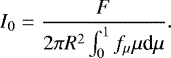
We included H, He, C, N, O, Na, Mg, Si, S, Ti, Fe, and Ni in the Cloudy simulation with solar abundance ratios, and computed the composition and ionisation structure of the atmosphere at the substellar point. The quiet Sun irradiance reference spectrum byWoods et al. (2009) is used to illuminate the planet in place of an HD 209458 SED, scaled to half the stellar luminosityto approximate integration over the planetary day side. The altitude scale of the atmosphere is determined iteratively as the composition evolves, according to
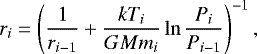 (1)
(1)
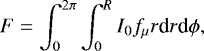
where ri is the radius of the ith layer (measured from the centre of the planet), k is the Boltzmann constant, Ti is the temperature of the ith layer, G is the gravitational constant, M is the planetary mass, mi is the mean molecular weight of particles at the ith layer, and Pi is the pressure of the ith layer. This process is iterated upon until the ionisation and altitude structures of the atmosphere change by less than 1% between iterations at all sampling points. Because Cloudy lacks the facility to include hydrodynamic effects and our framework does not account for the Roche potential, we limited the atmosphere to a maximum radius of 1 R⋆ (occurring at a pressure of approximately 2 × 10⁻¹² bar under the initial conditions). Outside of this radius, the atmospheric scale height diverges. Planetary and system parameters for HD 209458b are listed in Table 1; the final density profiles for individual species, as well as the input temperature profile, are presented in Fig. 1. Figure 2 presents the difference in the e− density for models with and without N, S, Ti, and Ni as a demonstration of the impact that adding additional elemental species into the model has on the atmospheric structure,
We again note that our model assumes hydrostatic equilibrium because Cloudy does not account for atmospheric escape, and we do not include the Roche potential due to stellar gravity. These assumptions are roughly valid below the sonic point and/or the Roche lobe boundary but invalid at higher altitudes. Our results therefore represent upper limits for atomic line core absorption that probe regions outside of the Roche lobe. The coupling of Cloudy to a model of atmospheric dynamics is subject to future work that will quantify the impact of escape and NLTE effects on detectable signatures.
HD 209458b planetary and system parameters.
2.2 Transmission spectrum
To obtain the transmission spectrum, we used Cloudy to compute the line-of-sight absorption and scattering of the stellar SED through the limb of the atmosphere at different altitudes. Our assumption of a spherically symmetric, static planetary atmosphere, the properties of which vary only with altitude, requires only a single Cloudy simulation to be computed at each impact parameter from the centre of the planet. Integrating these simulations around the line-of-sight axis in the azimuthal direction produces a series of concentric rings with constant transmission over any given ring, reducing the total number of simulations necessary to model the full transmission spectrum.
The 1D model properties are mapped onto concentric spherical shells, and path lengths through successive layers of atmosphere along line-of-sight chords are calculated as
 (2)
(2)
where li is the path length through the ith layer, ci is half the chord length along line of sight through the ith layer, ri is the radius of theith layer, and hi is the height down from the ith layer of the atmosphere to the chord altitude at the terminator. A schematic diagram of this geometry is displayed in Fig. 3. These lengths, along with the atmospheric properties of their respective layers, are stacked and entered into Cloudy, using the Cloudy “table” commands, as the line-of-sight transmission medium.
Cloudy computes output spectra spanning wavelengths from 29.98 m (10 MHz) to 12.40 fm (100 MeV) at a default spectral resolution of R = 300 for λ > 1.01 Å (<12.24 keV), and R = 33.333333 otherwise. We increased the output spectral resolution to R = 100 000 over a wavelength range of 920 Å < λ < 11 000 Å, while maintaining the default resolutions outside of this range. We selected these high-resolution boundaries to include a large number of Lyman series lines at the short wavelength end, and the HeI λ10 830 triplet at the long end. While the commonly accepted convention in spectroscopy is to use vacuum wavelengths for wavelengths shorter than 2000 Å and air wavelengths for wavelengths longer than 2000 Å, Cloudy outputs the full spectrum in vacuum wavelengths to avoid a discontinuity in the spectrum at 2000 Å. The output fromthe individual Cloudy transmission simulations is converted into the transmission spectrum by summing the contributions of the individual spectra, weighted by the relative area of the stellar disc they cover and the respective limb darkening.
We used a non-linear relation for stellar limb darkening (Claret 2000) of the form
 (3)
(3)
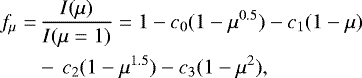
where I(μ) is the line-of-sight intensity at position μ = cosθ (θ is the angle between the line of sight and the emergent intensity) and c0, c1, c2, and c3 are the limb-darkening coefficients (Salz et al. 2019). The coefficients are derived by fitting stellar limb-darkening curves from a limb-darkened PHOENIX model with an effective temperature of Teff = 6100 K, surface gravity of log g = 4.5, and solar metallicity (Husser et al. 2013). We note that this PHOENIX model does not include computation of the stellar chromosphere or transition region, and is therefore incorrect in the estimation of centre-to-limb variations for emission lines forming in the stellar chromosphere and/or corona. The lack of chromospheric and coronal stellar emission also makes the PHOENIX model unsuitable for use as the central illumination source for the transmission spectrum because of the missing input high-energy stellar photons, which affect the planetary atmospheric composition, and because of the missing UV stellar emission lines. Conversely, observed solar limb spectra do not exist at high resolution for the full wavelength range considered in this work, making them unsuitable for limb-darkening calculations.
The wavelength dependence of the limb-darkening relation is accounted for by evaluating Eq. (3) every 1 Å (i.e. the sampling of the PHOENIX spectra) between 920 < λ < 11 000 Å. Example fits and residuals are presented in Fig. 4 for three different limb-darkening curves, one in the near-infrared (NIR), one in the visible (VIS), and one in the mid-ultraviolet (MUV).
The stellar disc is divided into rings, similar to the planetary atmosphere, every 0.01 R⋆ out to a maximum of 0.99 R⋆, and the limb darkening is evaluated independently for each ring. To generate the summation weights for building the transmission spectrum, we calculated the overlapping areas of the planetary and stellar rings using the general formula for two intersecting circles,
![\begin{multline*} A(r,R) = r^2\cos^{-1}\left[\frac{D^2+r^2-R^2}{2Dr}\right]+R^2\cos^{-1}\left[\frac{D^2+R^2-r^2}{2DR}\right] \\ -\frac{1}{2}\sqrt{(-D+r+R)(D+r-R)(D-r+R)(D+r+R)}\,, \end{multline*}](/articles/aa/full_html/2020/09/aa37672-20/aa37672-20-eq4.png) (4)
(4)
where A(r, R) is the area of the intersection, r and R are the radii of the two circles, respectively, and D is the distance between the centres of the circles. To convert these circular intersections to ring intersections, we subtracted the circular intersections of the next smaller ring radii from each of the planetary and stellar rings,
 (5)
(5)
where Aij is the overlapping area of planetary ring i and stellar ring j, ri is the radius of the ith planetary ring, and Rj is the radius of the jth stellar ring. An illustrative schematic of a planet in transit in this framework is presented in Fig. 5.
We then take the summation weights to be
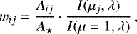 (6)
(6)
where wij is the weight of the overlapping ith and jth rings, Aij ∕A⋆ is the overlap area of the ith and jth rings relative to the area of the stellar disc, and I(μj, λ)∕I(μ = 1, λ) is the wavelength-dependent limb darkening of the jth ring. To build the relative flux transit spectrum out of the individual ring spectra, we assumed that the distance between the centres of the stellar and planetary discs is the impact parameter b (i.e. the planet is at mid transit), and the summation is performed according to
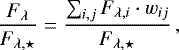 (7)
(7)
where Fλ is the in-transit flux spectrum, Fλ,⋆ is the out-of-transit stellar flux spectrum at disc centre, and Fλ,i is the flux spectrum of the ith planetary ring. The quiet Sun irradiance reference spectrum is a disc-integrated stellar spectrum and therefore already includes the average effect of stellar limb darkening. We extracted the intensity at disc centre by taking the definition of the disc-integrated spectrum
 (8)
(8)
where I0 = I(μ = 1) is the intensity at disc centre, r is the radial variable, ϕ is the azimuthal variable, and R is the stellarradius, and made the following change of variables:
 (9)
(9)
This results in an intensity at disc centre of
 (10)
(10)
The final transmission spectrum is generated by applying a transformation to the relative flux spectrum. The transformation is
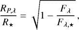 (11)
(11)
where RP,λ is the wavelength-dependent observed planetary radius and R⋆ is the stellar radius.
Figure 6 presents the resultant synthetic NLTE atomic transmission spectrum of HD 209458b at mid transit, computed for H, H2, He, Na, Mg, and Fe. The spectrum displays a large number of strong atomic absorption features, several of which extend to very high altitudes, namely the Lyman series and the MgII λ2800 Å doublet. There is evidence of strong FeII absorption around 2350 and 2600 Å, and a multitude of weak FeI lines spread across the majority of the full spectral range. The HeI λ10 830 Å triplet is present, as are both Hα and the Na D doublet.
Transit light curves are prepared using the same methodology as the transmission spectrum, while changing the value of D by adding an offset perpendicular to the impact parameter such that  , where x is the value of the offset. Relative flux spectra are evaluated over a range of values for x, simulating the planet transiting the disc of the star, and are then integrated over a given waveband or filter to produce the transit light curve. To demonstrate this process, we prepared synthetic light curves in a sample of five passbands (three wide and two narrow) spanning the full extent of our synthetic spectrum: the CUTE passband (~ 2550−3300 Å), the TESS passband (~6000−10 000 Å), the Kepler passband (~4350−9000 Å), a narrow Hα band (λ0 = 6562.8 Å, δλ ± 2.5 Å), and a narrow HeI λ10 830 band (λ0 = 10 830 Å, δλ ± 2.5 Å). The synthetic light curves are displayed in Fig. 7.
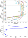 |
Fig. 1 HD 209458b 1D atmospheric model mixing ratios (top) and temperature profile (bottom). Mixing ratios are day-side averages calculated by Cloudy. The temperature profile is taken from Lavvas et al. (2014; lower) and Koskinen et al. (2013; upper), joined at 1 μbar (dashed greyline). The dots indicate the 200 points to which the T–P profile has been re-sampled. |
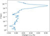 |
Fig. 2 Difference in modelled e− density, presented as the running mean over ten sampling points, for models that do and do not include N, S, Ti, and Ni. Models are otherwise equivalent. |
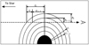 |
Fig. 3 Schematic diagram of transmission chords along the line of sight for transmission spectrum calculation. Here, c is half the chord length along line of sight, l is the path length through a given layer of atmosphere, h is the height down from the layer to the altitude of the transmission chord at the terminator, r is the radiusof the layer, and the subscripts denote the layers. |
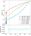 |
Fig. 4 PHOENIX model stellar limb-darkening curves (circles) and non-linear fits (lines), evaluated for three sample wavelengths, evaluated in 1 Å windows. Red: 9000 Å, green: 5000 Å, and blue: 2500 Å. The vertical grey line represents the largest radius we evaluate limb darkening at, 0.99 R⋆, equivalent to μ ≈ 0.14. |
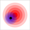 |
Fig. 5 Schematic diagram of the line-of-sight view of a transiting planet in our framework. The shaded red circles are the stellar rings of discrete limb darkening, the shaded blue circles are different layers of the planetary atmosphere, and the black circle is the bulk disc of the planet. |
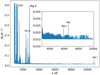 |
Fig. 6 High spectral resolution (R = 100 000) synthetic NLTE transmission spectrum of HD 209458b at mid transit. Prominent features include Lyman series lines, FeII packets of lines at ~2350 and 2600 Å, the MgII h&k doublet at 2800 Å, NaI D lines at 5890 Å, Hα, and the HeI triplet at ~10 830 Å. The inset displays the finer details of the 3000–10 000 Å range. |
3 Results
In this section, we present the effects of NLTE modelling on our synthetic spectrum, and compare our model spectrum with observed quantities for transit light curves and several strong spectral features. In all cases, synthetic quantities are presented with the same precision as the respective observations for ease of comparison. We confirm the modelled results of Oklopčić & Hirata (2018; HeI λ10 830 triplet), Fisher & Heng (2019; NaI D doublet), and Barman (2007; FeI optical continuum), and demonstrate that NLTE generally increases absorption of spectral features by up to 40% compared to LTE.
Notably, while the MgI λ2850 Å and MgII h&k lines are strong in our synthetic spectrum, recent publications of near-UV (NUV) observations for HD 209458b have shown that Mg is not detected in the upper atmosphere (Cubillos et al. 2020), suggesting that Mg-bearing aerosols are preferentially formed at lower altitudes and that the lower atmosphere is consequently not completely clear. Therefore, we leave Mg out of our comparative analysis here; a thorough discussion on the reasons for a non-detection of Mg in the upper atmosphere of HD 209458b is available in Cubillos et al. (2020).
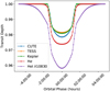 |
Fig. 7 Synthetic NLTE transit light curves in three wide and two narrow wavebands spanning the full synthetic spectral range: CUTE, TESS, Kepler, Hα, and HeI λ10 830. |
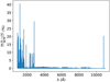 |
Fig. 8 Difference between NLTE and LTE synthetic spectra of HD 209458b at mid transit, at high spectral resolution (R = 100 000). |
3.1 LTE versus NLTE
In addition to the NLTE model spectrum, we produced an LTE spectrum following the same methodology described in Sect. 2. Cloudy’s method of LTE spectral synthesis only differs from the NLTE synthesis in that the former uses LTE-relative level populations instead of detailed level balance equations. All other aspects of the modelling, including photo-ionisation, are identical. We acknowledge that this is not true LTE, given that the ionisation is not calculated according tothe Saha equation, but we choose to call this model LTE in work to contrast with the NLTE model. Figure 8 compares our NLTE-relative flux spectrum with the LTE one. The average broadband NLTE effect is to increase the transit depth of atomic absorption lines by about 0.3% while preserving the shape of the lines in the optical and NIR. Larger differences are seen for specific lines in the NUV and far-UV (FUV), as well as for the HeI λ10 830 Å feature, with differences ranging between 1 and 20%. The large NLTE effect for the HeI triplet is not surprising given that these lines form through a primarily NLTE process.
The largest NLTE effects, which increase transit depths by > 20%, are seen in the Lyman series lines, the SiIII λ1206.5 Å line, the MgI λ2850 Å line, and the HeI λ10 830 triplet. The MgII h&k doublet, as well as the UV FeII groups of lines centred at ~ 2375 Å and ~ 2600 Å, show differences of ~ 10%. The remaining UV lines generally display changes of 5 to 15%, noticeably different from the VIS and NIR lines that show ≤1%. Notably, Hα is relatively unaffected by NLTE, as are the NaI D doublet lines; however, the Na lines display a curious behaviour where the wings of the lines show a larger difference than the line cores. Fisher & Heng (2019) likewise found that they were unable to distinguish between the LTE and NLTE line profiles of the Na doublet. The wings of Lyα are stronger in NLTE, but we are unable to comment upon the core of the line; a consequence of how we built our transmission spectrum is that lines are capped at a radius of R⋆, and Lyα extends to this limit in both the LTE and NLTE spectra. Regardless, interstellar absorption prevents testing the differences in the core of Lyα for all systems with the exception of those with the most extreme radial velocities. Figure 9 shows the effect of NLTE modelling on these features.
3.2 Broadband light curves
A comparison of our optical light curve transit depths with observed values is presented in Table 2. We find excellent agreement with the HST STIS G750M light curves, but it is the only HST configuration that produces a transit depth in agreement with our values. The remaining configurations produce transit depths deeper than those of our models, by more than 6σ in the case of the F550W grating. Conversely, our MOST model light curve is deeper by12σ than in the observations.
While we did include H2 Rayleigh scattering in our models, we ignored contributions from other molecular species and consequently underestimate the full effect. The mismatch between the observations and our modelled values may also be a consequence of our assumed planetary and stellar radii and of our planetary pressure-radius calibration. It is also possible that part of the difference can be ascribed to the use of different limb-darkening laws for the data analysis and the computation of the synthetic transit depths.
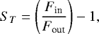
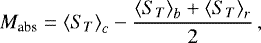
3.3 Na I D doublet
We compared the NaI D doublet lines in our spectra to those presented in Jensen et al. (2011) and Snellen et al. (2008). A total of 23 in-transit observations of the HD 209458b NaI D doublet and 69 out-of-transit observations were obtained by Jensen et al. (2011) using the Hobby-Eberly Telescope High Resolution Spectrograph (HET HRS; R = 65 000) and converted totransmission spectra according to
 (12)
(12)
where ST is the transmission spectrum flux normalised to 0, Fin is the observedin-transit flux, and Fout is the observed out-of-transit flux. They averaged the transmission spectra in three different 12 Å wavebands: a central waveband centred halfway between the cores of the two lines and two additional wavebands immediately to the blue and red of the central waveband. The total absorption level was then calculated as
 (13)
(13)
where Mabs is the measured absorption level and  ,
,  , and
, and  are the average absorption levels in the central, blue, and red wavebands, respectively. We calculated the absorption of our NaI D doublet in the same fashion, and present the results in Table 3. Additionally, we compared the peak absorption levels in the core of each line. Figure 10 displays the doublet in our models convolved to the resolution of HET HRS, highlighting the different 12 Å wavebands used in the analysis.
Our Na absorption is stronger in both our NLTE and LTE spectra than the observed value. The lack of pressure-broadened wings in ourmodel spectra artificially increases the absorption when measured in this fashion, which our higher overall absorption can be attributed to. While we find that our NLTE spectrum has deeper line cores than LTE, the LTE spectrum shows a greater overall absorption, attributed to the stronger wings of the doublet lines. Both the NLTE and LTE spectra show a ratio of the D1 to D2 core absorption values that agree within uncertainty with the observed ratio, although our line cores are deeper.
Snellen et al. (2008) collected 18 in-transit observations of the NaI D doublet observed with the Subaru High Dispersion Spectrograph (HDS; R = 45 000). They measured the depth of the NaI D features in the transmission spectrum within three spectral passbands, with widths of 0.75, 1.5, and 3.0 Å centred on each of the lines, and calculated the total absorption level as the central waveband minus the average of the blue and red wavebands, similar to above, and averaged the results of the separate lines. We again calculated the absorption of our NaI D doublet in the same fashion and present the results in Table 4. Figure 10 displays the doublet convolved to the resolution of Subaru’s HDS. Our derived absorption values are again stronger than those observed. This agrees with the previous analysis using 12 Å bands, where the models showed stronger absorption than observed, although the difference is not as large in these narrow bands.
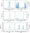 |
Fig. 9 NLTE−LTE differences for specific lines and features. Top-left: Lyα. Top-right: prominent FeI and FeII bands at NUV wavelengths. Middle-left: HeI λ10 830 Å triplet. Middle-right: MgI λ2852 Å line and MgII h&k lines. Bottom-left: Hα. Bottom-right: NaI D doublet. |
Broadband light curve transit depths at mid transit.
Absorption of the NaI D doublet and comparison with Jensen et al. (2011).
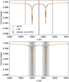 |
Fig. 10 NaI D doublet lines in our NLTE and LTE model spectra. Top: HET HRS comparison spectra (R = 65 000). The solid black line indicates the position centred between the two line cores and the dashed lines indicate the boundaries of the central 12 Å band. The black points indicate the observed core absorption of the lines. Bottom: Subaru HDS comparison spectra (R = 45 000). The shaded areas indicate the narrow (0.75 Å), medium (1.5 Å), and wide (3.0 Å) passbands used in the analysis. |
3.4 Hα
The HET HRS transmission spectroscopy observations of HD 209458b centred at the Hα line display an odd behaviour (Jensen et al. 2012). While the authors did not detect an overall absorption or “emission” signal over a 16 Å band centred on the stellar line core, they note that the average transmission spectrum shows a dramatic feature with a “spike” to the blue of the stellar line centre and a “dip” to the red. Both features peak at roughly 0.5% absolute deviation from zero and areseveral angstroms wide. The combined feature was also roughly symmetric when reflected about the zero point and line centre. While they do not report the signal-to-noise ratio for their observations, we note that our Hα lines both exhibit greater than 1% absorption in their cores, and would be detectable with similar observations.
We measured the absorption of our NLTE and LTE Hα lines according to Eq. (13), using 16 Å bands, and got absorption measurements of Mabs,NLTE = 0.0281% and Mabs,LTE = 0.0300%. We note that there are several additional lines within the 16 Å bands that are present in the NLTE spectrum but not the LTE spectrum, and highlight the fact that differences in the measured absorption is not uniquely caused by NLTE effects on Hα alone. A narrower 2 Å band reveals absorption measurements of Mabs,NLTE = 0.278% and Mabs,LTE = 0.249%, confirming that the stronger LTE absorption in the 16 Å band is caused by additional lines in the NLTE spectrum, and not limited to Hα. While we acknowledge the possibility that Cloudy lacks some relevant physics, one should also consider the possibility of problems in the data reduction and/or analysis that led to the odd shape of the transmission spectrum. Therefore, further observations and/or an independent re-analysis of the available data would be very valuable for providing additional constraints to the atmospheric properties of HD 209458b.
Absorption of the NaI D doublet and comparison with Snellen et al. (2008).
Absorption of the HeI λ10 830 Å triplet.
3.5 He I λ10 830 Å triplet
Alonso-Floriano et al. (2019) collected 33 observations of the HD 209458b HeI IR triplet in transmission with the CARMENES NIR channel. They took two measures of the strength of the planetary absorption, namely the peak value of the average absorption signal in the core of the two strongest and blended lines, and the average value over a 0.3 Å bandwidth centred on the core of the feature. We took the same measures of both our NLTE and LTE spectra, after convolving them to the spectral resolution of CARMENES NIR (R = 80 400), and present the results in Table 5. Our NLTE and LTE line profiles are displayed in Fig. 11.
Neither the NLTE nor the LTE values agree with the observations for either measure, with the NLTE model showing stronger absorption than observed by ~3.6% and the LTE showing weaker absorption by ~0.6%. We additionally investigated the ratio of the core absorption to the absorption over the 0.3 Å band and find that our models both exhibit ratios larger than the observed value, suggesting narrower line profiles than observed. This indicates that either the 1D atmospheric model temperature profile is too cool at the altitudes where HeI absorption is optically thick, or that we are missing an additional source of broadening, such as microturbulence, in our modelling.
In Oklopčić & Hirata (2018), the authors develop a simple 1D model of an escaping atmosphere comprised of only H and He, and predict the absorption of the HeI λ10 830 triplet lines. They assume the planet transits the centre of the stellar disc and do not include limb darkening in their model. For an HD 209458b-like planet under these assumptions, they predict depths in the line cores of 0.44 and 2.38% for the weak and strong lines,respectively, and a combined equivalent width (EW) of the feature of 0.014 Å. Using the same set of assumptionsto prepare an NLTE transmission spectrum with Cloudy, we find depths of 0.38 and 2.55% and an EW of 0.012 Å, in line with the predictions of Oklopčić & Hirata (2018). The agreement between our model and that of Oklopčić & Hirata (2018), which describes in detail the excitation chemistry, is an important benchmark. This agreement gives us confidence in the capability of Cloudy to model theoretical planetary atmospheres and transmission spectra.
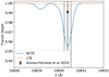 |
Fig. 11 HeI λ10 830 triplet lines in our NLTE and LTE model spectra. The solid black line indicates the position of the core of the strong blended feature, the dashed lines indicate a 0.3 Å band centred on the line core, and the black point indicates the observed level of core absorption. |
3.6 Fe I and Fe II
We compared our model spectra to three archival NUV Fe-band transmission observations of HD 209458b, obtained with HST STIS (Vidal-Madjar et al. 2013) using the E230M grating. The data consist of échelle spectra comprising 23 orders, each of which contain 1024 wavelength samples, with a spectral resolution of R = 30 000. The entire STIS spectrum covers the 2300−3100 Å range, withsome overlap between the orders. We treated the synthetic spectra as in Cubillos et al. (2020), re-sampling the spectrum at a resolution ofR = 12 000. We find that our NLTE spectrum generally provides a better fit to the observations, thus we focus on the NLTE comparison here. Figure 12 displays the observed spectra, overlayed with our NLTE model spectrum at both the Cloudy output high resolution and convolved to the observed resolution.
We note that our model fits the strength of the FeII band centred at 2600 Å more accurately than the one centred at 2375 Å; our models show similar line strengths in the two bands, while the observed data show stronger absorption in the 2375 Å band. This effect of the two bands having different line strengths has also been observed to occur in the NUV transmission spectrum of WASP-121b(Sing et al. 2019). This difference is unexpected because the relative strength of the two bands is controlled by atomic line parameters, the quality of which has been confirmed by comparisons with spectra of well-studied stars (Landstreet 2011). One possible explanation for why our model produces this behaviour is that Cloudy usessuper-levels to compute NLTE level populations for ions more complicated than the H-like and He-like iso-electronic sequences. Super-levels are the higher energy levels in model atoms grouped together into a single level or a few representative levels, usually one per principle quantum number. While FeI and II are both extremely complicated atoms to model for detailed NLTE calculations, current model atoms are being constantly improved (e.g. Bautista et al. 2017), making the use of super-levels a simplifying approximation rather than a necessity.
Barman (2007) demonstrated that the slope of the optical continuum in the range of λ ≈ 3000 to 6000 Å could be reproduced at low spectral resolution (R ~ 5000) in a cloudless atmosphere as a result of metallic line blanketing, primarily FeI lines. We compare our NLTE spectrum with HST STIS G750M, G750L, and G430L observations of HD 209458b (Sing et al. 2016), and the LTE spectral model of Fortney et al. (2010). The observations were made at a spectral resolution of R ~ 5540 and binned with a variable bin size depending on the STIS grating. Our high-resolution spectrum displays stronger continuum absorption than either the observed data or model, which can be attributed to differences in the values used for the planetary and stellar radii. We consequently matched our continuum level to the modelled level at 9300 Å, shifting our spectrum down by ΔRp∕R⋆ = −0.00223. Figure 13 displays our NLTE spectrum comparison with the model and observations. We find that the continuum level in the high-resolution spectrum is indeed weaker than both the predicted and observed levels; however, when convolved to the spectral resolution of and binned in the same manner as the observations, our synthetic spectrum that accounts for both H2 Rayleigh scattering and FeI line blanketing is able to reproduce the slope of the continuum in this region, with the exception of two features.
As discussed in Sect. 2, Cloudy does not include pressure broadening of lines in its spectral synthesis, and the wings of our NaI D doublet are much weaker than observed. Additionally, we display a strong broadband absorption feature centred at ~3750 Å that is not present in the observations. While the placement of the feature would suggest that it is related to the Ca II H and K lines, this is coincidental as our model does not include Ca. The feature is the result of blending many atomic absorption lines, the majority of which are FeI. When considering the FeI and FeII features in the NUV and optical together, it appears that an atmosphere in which Fe is more ionised than our model below the 1 μbar level may be a better fit to the data. In fact, this would lead to weaker absorption around 3750 Å and stronger absorption at the position of the FeII NUV bands.
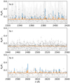 |
Fig. 12 NUV FeI & II bands. The grey points with error bars denote the observed spectrum at a resolution of R ~ 12 000, the blue curve is our high-resolution NLTE spectrum, and the orange curve is our spectrum convolved to the resolution of the observed data. Top and bottom panels: bands of prominent FeII lines and the middle panel shows a band of FeI lines. |
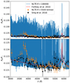 |
Fig. 13 Comparison of the optical continuum slope between our NLTE spectrum and observations. Top: full region, displaying the strength of high-resolution atomic features. Bottom: zoomed view of the continuum level in this region. |
3.7 C, O, and Si UV Lines
Far-ultraviolet observations of HD 209458b have been performed with both the HST STIS G140L low-resolution grating (R ~ 600; Vidal-Madjar et al. 2004) and the HST COS G130M high-resolution grating (R ~ 17 000–20 000; Linsky et al. 2010; Ballester & Ben-Jaffel 2015). While there is some debate over the observability and detection of a number of FUV diagnostic lines, we chose four to focus on: SiIII λ1206, OI λ1302, CII λ1335, and SiII λ1527.
Vidal-Madjar et al. (2004) fitted the observed transit light curves in narrow windows (~10 Å) centred on the target lines, leaving  as a free parameter in their fit and recording the fitted value as their measure of the absorption for these lines. Table 6 compares their values with the values derived in a similar manner from our NLTE and LTE spectra. While they present strong detections of the CII and OI features, both of their Si features are consistent with non-detections. In these cases, they reported the 2σ upper limits on the absorption depths. Our measured values agree with the observations and upper limits in all cases except for OI λ1302, where we find less absorption than the observations by greater than 2σ; however, it should be noted that these comparisons do not account for interstellar medium absorption affecting the shortest wavelength lines of the OI triplet and CII doublet.
Both Linsky et al. (2010) and Ballester & Ben-Jaffel (2015) measured the absorption as the average ratio of the in- to out-of-transit fluxes in a ± 50 km s−1 window centred on the lines, although Ballester & Ben-Jaffel (2015) claim that the Linsky et al. (2010) results are invalid for not recording the stellar flux at the time of their observations, and for including errors for photon noise only, ignoring the intra-transit variations instellar flux. Results from both are presented in Table 7, alongside absorption values computed in a similar fashion from our NLTE and LTE spectra. While the Ballester & Ben-Jaffel (2015) results show stronger absorption for the CII λ1335 doublet, their SiIII λ1206 absorption is consistent with a non-detection, and both measurements exhibit uncertainties greater than those of Linsky et al. (2010) by factors of ~6.5. Our measured values agree with all the observed values, with the exception of SiIII λ1206 in our NLTE spectrum, which was weaker than the result reported by Linsky et al. (2010). The comparison for the CII λ1335 doublet has to be taken with care because our transmission spectra do not account for interstellar medium absorption. When considering just the line at a longer wavelength, which is not affected by the interstellar medium, weobtain an absorption of 11.0% in NLTE and 11.1% in LTE, while the observed absorption is 7.9±1.5% (Linsky et al. 2010).
4 Conclusions
We have presented a generalised framework for producing synthetic transmission spectra of exoplanets, given a planetary T–P profile as input, using the NLTE spectral synthesis hydrostatic code Cloudy. The framework is designed to work for a broad range of exoplanetary atmospheric conditions and to produce transmission spectra at a desired spectral resolution in a given waveband, with the possibility to account for stellar limb darkening. To demonstrate our framework, we generated both an LTE and NLTE transmission spectrum for the well-studied exoplanet HD 209458b, starting from a published planetary T–P profile that accounts for hydrodynamics.
We presented a differential comparison of the NLTE and LTE spectra, highlighting prominent features with strong NLTE effects. We also performed comparisons with observed broadband transit light curves, the NaI D doublet, Hα, the HeI λ10 830 triplet, FeI and FeII bands in both the UV and optical, and several FUV lines including SiIII λ1206, the OI λ1302 triplet, the CII λ1335 doublet, and SiII λ1527.
Our simulations match one out of five observed broadband transit depths and the mismatch may be caused by one or a combinationof the following: the lack of molecular absorption and aerosols in the transmission spectra; differences in the assumed planetary and stellar radii; the adopted planetary pressure-radius calibration; and differences in the considered limb-darkening laws. Both our NLTE and LTE spectra show stronger total absorption than observed at the position of the NaI D lines, but the comparison is biased by the fact that our model does not account for pressure broadening. Our measured absorption values for the FUV lines agree with observations for three of the four lines, but are weaker than the observed OI λ1302 absorption.
We were unable to compare our synthetic Hα absorption with observations because of the odd behaviour present in the observed spectrum, but we note that the strength of our line should be observable, given the noise level of the observations. We suggest that further Hα observations and/or an independent re-analysis of the existing ones should be carried out to clarify the presence and possible strength of this feature.
Neither our NLTE nor our LTE spectra match the observed HeI λ10 830 absorption, with our NLTE model overestimating the absorption by ~ 3.6%, and our LTE model underestimating the absorption by ~0.6%. Additionally, we find that our line profiles are narrower than the observed lines, suggesting either that the temperature profile in the atmospheric model is too cool in the region where HeI becomes optically thick; that the excitation chemistry needs to be revised; that we are missing an additional source of broadening such as microturbulence; or some combination of the above. We were able to reproduce the predicted absorption of HeI λ10 830 under the same set of assumptions as Oklopčić & Hirata (2018).
We find differences up to the 10% level between our LTE and NLTE spectra of the NUV FeI & II bands, with the NLTE spectrum being a better fit to the data. Both LTE and NLTE models fit the FeII λ2600 band better than the λ2375 band, where we underestimate the absorption. We confirm the result of Barman (2007) that the slope of the optical continuum can be reproduced in low-resolution spectra by FeI line blanketing and H2 Rayleigh scattering without additional absorption. We propose that additional Fe ionisation below the 1 μbar level in our model would provide better fits to the data in both the optical and UV.
A differential comparison of our model spectra revealed that NLTE modelling generally increases the absorption of features by ≤ 1% in the optical and NIR, and 5–20% in the UV, but can increase absorption by up to ~40% for individual features (e.g. the MgI λ2850 or SiIII λ1206.5 lines). We found negligible difference between LTE and NLTE for both Hα and the NaID doublet. We have benchmarked this application of Cloudy by reproducing the results of Oklopčić & Hirata (2018), Fisher & Heng (2019), and Barman (2007) for HeI λ10 830, NaI D, and optical FeI continuum absorption, respectively. We conclude that accounting for NLTE effects is necessary for modelling planetary spectral lines that form in the upper atmosphere, particularly at UV wavelengths.
The modelling framework is open to several improvements. Currently, the inclusion of any of the following would improve the physical realism of the model: hydrodynamics, molecular chemistry, pressure broadening, 3D atmospheric structure, stellar activity, andDoppler effects. While Cloudy lacks the ability to include hydrodynamics, pressure broadening, and 3D structure in our framework, it is possible to include stellar activity and Doppler effects by making several additional assumptions and knowledge of additional planetary and stellar parameters.
HST STIS G140L low-resolution absorption depths for UV spectral lines, measured as  in a narrow window around the lines.
HST COS G130M high-resolution absorption depths for UV spectral lines, measured as the ratio of in- to out-of-transit flux in a ± 50 km s−1 centred on the lines.
Acknowledgements
This research has made use of the Extrasolar Planet Encyclopaedia, the Exoplanet Transit Database (Poddaný et al. 2010), NASA’s Astrophysics Data System Bibliographic Services, the NASA Exoplanet Archive, which is operated by the California Institute of Technology, under contract with the National Aeronautics and Space Administration under the Exoplanet Exploration Program, and the SVO Filter Profile Service (http://svo2.cab.inta-csic.es/theory/fps/) supported from the Spanish MINECO through grant AYA2017-84089. This research also made use of the NIST Atomic Spectra Database funded [in part] by NIST’s Standard Reference Data Program (SRDP) and by NIST’s Systems Integration for Manufacturing Applications (SIMA) Program. M.E.Y. acknowledges funding from the ÖAW-Innovationsfonds IF_2017_03. The following software and packages were used in this work: Cloudy v17.01 (Ferland et al. 2017); Python v2.7; Python packages Astropy (Astropy Collaboration 2013), NumPy (Oliphant 2006; van der Walt et al. 2011), and Matplotlib (Hunter 2007).
References
- Agol, E., & Steffen, J. H. 2007, MNRAS, 374, 941 [Google Scholar]
- Ahlers, J. P., Barnes, J. W., & Barnes, R. 2015, ApJ, 814, 67 [NASA ADS] [CrossRef] [Google Scholar]
- Alonso-Floriano, F. J., Snellen, I. A. G., Czesla, S., et al. 2019, A&A, 629, A110 [NASA ADS] [CrossRef] [EDP Sciences] [Google Scholar]
- Astropy Collaboration (Robitaille, T. P., et al.) 2013, A&A, 558, A33 [NASA ADS] [CrossRef] [EDP Sciences] [Google Scholar]
- Ballester, G. E., & Ben-Jaffel, L. 2015, ApJ, 804, 116 [Google Scholar]
- Barman, T. 2007, ApJ, 661, L191 [Google Scholar]
- Barman, T. S., Hauschildt, P. H., Schweitzer, A., et al. 2002, ApJ, 569, L51 [Google Scholar]
- Barnes, J. W. 2009, ApJ, 705, 683 [Google Scholar]
- Bautista, M. A., Lind, K., & Bergemann, M. 2017, A&A, 606, A127 [NASA ADS] [CrossRef] [EDP Sciences] [Google Scholar]
- Bourrier, V., Lecavelier des Etangs, A., Ehrenreich, D., et al. 2018, A&A, 620, A147 [NASA ADS] [CrossRef] [EDP Sciences] [Google Scholar]
- Brogi, M., de Kok, R. J., Albrecht, S., et al. 2016, ApJ, 817, 106 [Google Scholar]
- Charbonneau, D., Brown, T. M., Latham, D. W., & Mayor, M. 2000, ApJ, 529, L45 [Google Scholar]
- Charbonneau, D., Brown, T. M., Noyes, R. W., & Gilliland, R. L. 2002, ApJ, 568, 377 [NASA ADS] [CrossRef] [Google Scholar]
- Claret, A. 2000, A&A, 363, 1081 [NASA ADS] [Google Scholar]
- Colón, K. D., Ford, E. B., Redfield, S., et al. 2012, MNRAS, 419, 2233 [Google Scholar]
- Cubillos, P. E., Fossati, L., Koskinen, T., et al. 2020, AJ, 159, 111 [Google Scholar]
- del Burgo, C., & Allende Prieto C. 2016, MNRAS, 463, 1400 [Google Scholar]
- Deming, D., Wilkins, A., McCullough, P., et al. 2013, ApJ, 774, 95 [Google Scholar]
- dos Santos, L. A., Ehrenreich, D., Bourrier, V., et al. 2020, A&A 634, L4 [EDP Sciences] [Google Scholar]
- Ehrenreich, D., Bourrier, V., Wheatley, P. J., et al. 2015, Nature, 522, 459 [Google Scholar]
- Espinoza, N., Rackham, B. V., Jordán, A., et al. 2019, MNRAS, 482, 2065 [Google Scholar]
- Evans, T. M., Aigrain, S., Gibson, N., et al. 2015, MNRAS, 451, 680 [Google Scholar]
- Ferland, G. J., Chatzikos, M., Guzmán, F., et al. 2017, Rev. Mex. Astron. Astrofis., 53, 385 [NASA ADS] [Google Scholar]
- Fisher, C., & Heng, K. 2019, ApJ, 881, 25 [Google Scholar]
- Fortney, J. J., Sudarsky, D., Hubeny, I., et al. 2003, ApJ, 589, 615 [Google Scholar]
- Fortney, J. J., Shabram, M., Showman, A. P., et al. 2010, ApJ, 709, 1396 [NASA ADS] [CrossRef] [Google Scholar]
- Fossati, L., Haswell, C. A., Froning, C. S., et al. 2010, ApJ, 714, L222 [Google Scholar]
- Fraine, J., Deming, D., Benneke, B., et al. 2014, Nature, 513, 526 [Google Scholar]
- Haswell, C. A., Fossati, L., Ayres, T., et al. 2012, ApJ, 760, 79 [Google Scholar]
- Henry, G. W., Marcy, G. W., Butler, R. P., & Vogt, S. S. 2000, ApJ, 529, L41 [Google Scholar]
- Hunter, J. D. 2007, Comput. Sci. Eng., 9, 90 [NASA ADS] [CrossRef] [Google Scholar]
- Husser, T. O., Wende-von Berg, S., Dreizler, S., et al. 2013, A&A, 553, A6 [NASA ADS] [CrossRef] [EDP Sciences] [Google Scholar]
- Jensen, A. G., Redfield, S., Endl, M., et al. 2011, ApJ, 743, 203 [Google Scholar]
- Jensen, A. G., Redfield, S., Endl, M., et al. 2012, ApJ, 751, 86 [Google Scholar]
- Koskinen, T. T., Harris, M. J., Yelle, R. V., & Lavvas, P. 2013, Icarus, 226, 1678 [Google Scholar]
- Kreidberg, L., Line, M. R., Bean, J. L., et al. 2015, ApJ, 814, 66 [NASA ADS] [CrossRef] [Google Scholar]
- Landstreet, J. D. 2011, A&A, 528, A132 [NASA ADS] [CrossRef] [EDP Sciences] [Google Scholar]
- Lavvas, P., Koskinen, T., & Yelle, R. V. 2014, ApJ, 796, 15 [Google Scholar]
- Lecavelier Des Etangs, A., Ehrenreich, D., Vidal-Madjar, A., et al. 2010, A&A, 514, A72 [NASA ADS] [CrossRef] [EDP Sciences] [Google Scholar]
- Linsky, J. L., Yang, H., France, K., et al. 2010, ApJ, 717, 1291 [Google Scholar]
- Masuda, K. 2015, ApJ, 805, 28 [NASA ADS] [CrossRef] [Google Scholar]
- Mazeh, T., Naef, D., Torres, G., et al. 2000, ApJ, 532, L55 [NASA ADS] [CrossRef] [PubMed] [Google Scholar]
- McCullough, P. R., Crouzet, N., Deming, D., & Madhusudhan, N. 2014, ApJ, 791, 55 [NASA ADS] [CrossRef] [Google Scholar]
- Nortmann, L., Pallé, E., Salz, M., et al. 2018, Science, 362, 1388 [Google Scholar]
- Nugroho, S. K., Kawahara, H., Masuda, K., et al. 2017, AJ, 154, 221 [NASA ADS] [CrossRef] [Google Scholar]
- Oklopčić, A., & Hirata, C. M. 2018, ApJ, 855, L11 [Google Scholar]
- Oliphant, T. E. 2006, A guide to NumPy, (USA: Trelgol Publishing), 1 [Google Scholar]
- Parmentier, V., Line, M. R., Bean, J. L., et al. 2018, A&A, 617, A110 [NASA ADS] [CrossRef] [EDP Sciences] [Google Scholar]
- Poddaný, S., Brát, L., & Pejcha, O. 2010, New Astron., 15, 297 [NASA ADS] [CrossRef] [Google Scholar]
- Redfield, S., Endl, M., Cochran, W. D., & Koesterke, L. 2008, ApJ, 673, L87 [NASA ADS] [CrossRef] [MathSciNet] [Google Scholar]
- Rodler, F., Kürster, M., & Barnes, J. R. 2013, MNRAS, 432, 1980 [NASA ADS] [CrossRef] [Google Scholar]
- Rowe, J. F., Matthews, J. M., Seager, S., et al. 2008, ApJ, 689, 1345 [NASA ADS] [CrossRef] [Google Scholar]
- Salz, M., Banerjee, R., Mignone, A., et al. 2015, A&A, 576, A21 [NASA ADS] [CrossRef] [EDP Sciences] [Google Scholar]
- Salz, M., Czesla, S., Schneider, P. C., et al. 2018, A&A, 620, A97 [NASA ADS] [CrossRef] [EDP Sciences] [Google Scholar]
- Salz, M., Schneider, P. C., Fossati, L., et al. 2019, A&A, 623, A57 [NASA ADS] [CrossRef] [EDP Sciences] [Google Scholar]
- Sánchez-López, A., Alonso-Floriano, F. J., López-Puertas, M., et al. 2019, A&A, 630, A53 [NASA ADS] [CrossRef] [EDP Sciences] [Google Scholar]
- Schlawin, E., Agol, E., Walkowicz, L. M., Covey, K., & Lloyd, J. P. 2010, ApJ, 722, L75 [NASA ADS] [CrossRef] [Google Scholar]
- Showman, A. P., Fortney, J. J., Lian, Y., et al. 2009, ApJ, 699, 564 [NASA ADS] [CrossRef] [Google Scholar]
- Sing, D. K., Désert, J. M., Fortney, J. J., et al. 2011, A&A, 527, A73 [NASA ADS] [CrossRef] [EDP Sciences] [Google Scholar]
- Sing, D. K., Fortney, J. J., Nikolov, N., et al. 2016, Nature, 529, 59 [NASA ADS] [CrossRef] [Google Scholar]
- Sing, D. K., Lavvas, P., Ballester, G. E., et al. 2019, AJ, 158, 91 [Google Scholar]
- Snellen, I. A. G., Albrecht, S., de Mooij, E. J. W., & Le Poole R. S. 2008, A&A, 487, 357 [NASA ADS] [CrossRef] [EDP Sciences] [Google Scholar]
- Snellen, I. A. G., de Kok, R. J., de Mooij, E. J. W., & Albrecht, S. 2010, Nature, 465, 1049 [NASA ADS] [CrossRef] [PubMed] [Google Scholar]
- Stassun, K. G., Collins, K. A., & Gaudi, B. S. 2017, AJ, 153, 136 [NASA ADS] [CrossRef] [Google Scholar]
- Turner, J. D., de Mooij, E. J. W., Jayawardhana, R., et al. 2020, ApJ, 888, L13 [NASA ADS] [CrossRef] [Google Scholar]
- van der Walt, S., Colbert, S. C., & Varoquaux, G. 2011, Comput. Sci. Eng., 13, 22 [Google Scholar]
- Vidal-Madjar, A., Lecavelier des Etangs, A., Désert, J. M., et al. 2003, Nature, 422, 143 [NASA ADS] [CrossRef] [PubMed] [Google Scholar]
- Vidal-Madjar, A., Désert, J. M., Lecavelier des Etangs, A., et al. 2004, ApJ, 604, L69 [NASA ADS] [CrossRef] [Google Scholar]
- Vidal-Madjar, A., Huitson, C. M., Bourrier, V., et al. 2013, A&A, 560, A54 [NASA ADS] [CrossRef] [EDP Sciences] [Google Scholar]
- Woods, T. N., Chamberlin, P. C., Harder, J. W., et al. 2009, Geophys. Res. Lett., 36, L01101 [NASA ADS] [CrossRef] [Google Scholar]
- Wood, P. L., Maxted, P. F. L., Smalley, B., & Iro, N. 2011, MNRAS, 412, 2376 [NASA ADS] [CrossRef] [Google Scholar]
- Yan, F., & Henning, T. 2018, Nat. Astron., 2, 714 [NASA ADS] [CrossRef] [Google Scholar]
- Yan, F., Casasayas-Barris, N., Molaverdikhani, K., et al. 2019, A&A 632, A69 [NASA ADS] [CrossRef] [EDP Sciences] [Google Scholar]
All Tables
HST STIS G140L low-resolution absorption depths for UV spectral lines, measured as in a narrow window around the lines.
HST COS G130M high-resolution absorption depths for UV spectral lines, measured as the ratio of in- to out-of-transit flux in a ± 50 km s−1 centred on the lines.
All Figures
|
Fig. 1 HD 209458b 1D atmospheric model mixing ratios (top) and temperature profile (bottom). Mixing ratios are day-side averages calculated by Cloudy. The temperature profile is taken from Lavvas et al. (2014; lower) and Koskinen et al. (2013; upper), joined at 1 μbar (dashed greyline). The dots indicate the 200 points to which the T–P profile has been re-sampled. |
| In the text | |
|
Fig. 2 Difference in modelled e− density, presented as the running mean over ten sampling points, for models that do and do not include N, S, Ti, and Ni. Models are otherwise equivalent. |
| In the text | |
|
Fig. 3 Schematic diagram of transmission chords along the line of sight for transmission spectrum calculation. Here, c is half the chord length along line of sight, l is the path length through a given layer of atmosphere, h is the height down from the layer to the altitude of the transmission chord at the terminator, r is the radiusof the layer, and the subscripts denote the layers. |
| In the text | |
|
Fig. 4 PHOENIX model stellar limb-darkening curves (circles) and non-linear fits (lines), evaluated for three sample wavelengths, evaluated in 1 Å windows. Red: 9000 Å, green: 5000 Å, and blue: 2500 Å. The vertical grey line represents the largest radius we evaluate limb darkening at, 0.99 R⋆, equivalent to μ ≈ 0.14. |
| In the text | |
|
Fig. 5 Schematic diagram of the line-of-sight view of a transiting planet in our framework. The shaded red circles are the stellar rings of discrete limb darkening, the shaded blue circles are different layers of the planetary atmosphere, and the black circle is the bulk disc of the planet. |
| In the text | |
|
Fig. 6 High spectral resolution (R = 100 000) synthetic NLTE transmission spectrum of HD 209458b at mid transit. Prominent features include Lyman series lines, FeII packets of lines at ~2350 and 2600 Å, the MgII h&k doublet at 2800 Å, NaI D lines at 5890 Å, Hα, and the HeI triplet at ~10 830 Å. The inset displays the finer details of the 3000–10 000 Å range. |
| In the text | |
|
Fig. 7 Synthetic NLTE transit light curves in three wide and two narrow wavebands spanning the full synthetic spectral range: CUTE, TESS, Kepler, Hα, and HeI λ10 830. |
| In the text | |
|
Fig. 8 Difference between NLTE and LTE synthetic spectra of HD 209458b at mid transit, at high spectral resolution (R = 100 000). |
| In the text | |
|
Fig. 9 NLTE−LTE differences for specific lines and features. Top-left: Lyα. Top-right: prominent FeI and FeII bands at NUV wavelengths. Middle-left: HeI λ10 830 Å triplet. Middle-right: MgI λ2852 Å line and MgII h&k lines. Bottom-left: Hα. Bottom-right: NaI D doublet. |
| In the text | |
|
Fig. 10 NaI D doublet lines in our NLTE and LTE model spectra. Top: HET HRS comparison spectra (R = 65 000). The solid black line indicates the position centred between the two line cores and the dashed lines indicate the boundaries of the central 12 Å band. The black points indicate the observed core absorption of the lines. Bottom: Subaru HDS comparison spectra (R = 45 000). The shaded areas indicate the narrow (0.75 Å), medium (1.5 Å), and wide (3.0 Å) passbands used in the analysis. |
| In the text | |
|
Fig. 11 HeI λ10 830 triplet lines in our NLTE and LTE model spectra. The solid black line indicates the position of the core of the strong blended feature, the dashed lines indicate a 0.3 Å band centred on the line core, and the black point indicates the observed level of core absorption. |
| In the text | |
|
Fig. 12 NUV FeI & II bands. The grey points with error bars denote the observed spectrum at a resolution of R ~ 12 000, the blue curve is our high-resolution NLTE spectrum, and the orange curve is our spectrum convolved to the resolution of the observed data. Top and bottom panels: bands of prominent FeII lines and the middle panel shows a band of FeI lines. |
| In the text | |
|
Fig. 13 Comparison of the optical continuum slope between our NLTE spectrum and observations. Top: full region, displaying the strength of high-resolution atomic features. Bottom: zoomed view of the continuum level in this region. |
| In the text | |
Current usage metrics show cumulative count of Article Views (full-text article views including HTML views, PDF and ePub downloads, according to the available data) and Abstracts Views on Vision4Press platform.
Data correspond to usage on the plateform after 2015. The current usage metrics is available 48-96 hours after online publication and is updated daily on week days.
Initial download of the metrics may take a while.