| Issue |
A&A
Volume 640, August 2020
|
|
|---|---|---|
| Article Number | L5 | |
| Number of page(s) | 9 | |
| Section | Letters to the Editor | |
| DOI | https://doi.org/10.1051/0004-6361/202038294 | |
| Published online | 29 July 2020 | |
Letter to the Editor
A temperature inversion with atomic iron in the ultra-hot dayside atmosphere of WASP-189b⋆
1
Institut für Astrophysik, Georg-August-Universität, Friedrich-Hund-Platz 1, 37077 Göttingen, Germany
e-mail: This email address is being protected from spambots. You need JavaScript enabled to view it.
2
Instituto de Astrofísica de Canarias (IAC), Calle Vía Lactea s/n, 38200 La Laguna, Tenerife, Spain
3
Departamento de Astrofísica, Universidad de La Laguna, 38026 La Laguna, Tenerife, Spain
4
Max-Planck-Institut für Astronomie, Königstuhl 17, 69117 Heidelberg, Germany
5
Key Laboratory of Planetary Sciences, Purple Mountain Observatory, Chinese Academy of Sciences, Nanjing 210023, PR China
Received:
29
April
2020
Accepted:
3
July
2020
Abstract
Temperature inversion layers are predicted to be present in ultra-hot giant planet atmospheres. Although such inversion layers have recently been observed in several ultra-hot Jupiters, the chemical species responsible for creating the inversion remain unidentified. Here, we present observations of the thermal emission spectrum of an ultra-hot Jupiter, WASP-189b, at high spectral resolution using the HARPS-N spectrograph. Using the cross-correlation technique, we detect a strong Fe I signal. The detected Fe I spectral lines are found in emission, which is direct evidence of a temperature inversion in the planetary atmosphere. We further performed a retrieval on the observed spectrum using a forward model with an MCMC approach. When assuming a solar metallicity, the best-fit result returns a temperature of 4320−100+120 K at the top of the inversion, which is significantly hotter than the planetary equilibrium temperature (2641 K). The temperature at the bottom of the inversion is determined as 2200−800+1000 K. Such a strong temperature inversion is probably created by the absorption of atomic species like Fe I.
Key words: planets and satellites: atmospheres / techniques: spectroscopic / planets and satellites: individual: WASP-189b
The combined residual spectrum in Fig. B.1 is only available at the CDS via anonymous ftp to cdsarc.u-strasbg.fr (130.79.128.5) or via http://cdsarc.u-strasbg.fr/viz-bin/cat/J/A+A/640/L5
© ESO 2020
1. Introduction
Characterising exoplanet atmospheres is an expanding and quickly evolving subject within the exoplanet field. One of the key properties of an atmosphere is its temperature structure. Ultra-hot giant planets with equilibrium temperatures (Teq) larger than 2000 K have been proposed to possess a temperature inversion (i.e. a stratospheric layer where temperature increases with altitude), because of the strong absorption of titanium oxide (TiO) and vanadium oxide (VO) in their atmospheres (Hubeny et al. 2003; Fortney et al. 2008).
Earlier searches for temperature inversions and TiO/VO were mostly made at low spectral resolutions. Although there are claims or evidence of inversions and TiO detections (e.g. Knutson et al. 2008; Désert et al. 2008; Todorov et al. 2010; O’Donovan et al. 2010; Sedaghati et al. 2017), many of them are the subject of debate (e.g. Charbonneau et al. 2008; Zellem et al. 2014; Diamond-Lowe et al. 2014; Schwarz et al. 2015; Line et al. 2016; Espinoza et al. 2019). Haynes et al. (2015) observed the thermal emission spectrum of an ultra-hot Jupiter (UHJ), WASP-33b, and found evidence of a temperature inversion. The existence of an inversion in WASP-33b was later confirmed by Nugroho et al. (2017) with a detection of TiO lines in emission line shape using high-resolution spectroscopy. A temperature inversion has also been detected in another UHJ, WASP-121b, by Evans et al. (2017). The latter authors observed the low-resolution thermal emission spectrum of WASP-121b and detected an emission feature of H2O. However, Merritt et al. (2020) searched for TiO and VO in WASP-121b using high-resolution spectroscopy and reported a non-detection of TiO and VO. In addition, signs of thermal inversions, which are inferred from excess emission due to CO at the 4.5 μm photometry band of the Spitzer telescope, have been observed in several UHJs including WASP-18b (Sheppard et al. 2017; Arcangeli et al. 2018) and WASP-103b (Kreidberg et al. 2018).
Recent theoretical simulations predict that atomic metals like Fe and Mg can exist in the atmosphere of UHJs (e.g. Parmentier et al. 2018; Kitzmann et al. 2018; Helling et al. 2019), and the absorption of these metal lines at optical and UV wavelengths is capable of producing temperature inversions without the presence of TiO/VO (Lothringer et al. 2018). Lothringer & Barman (2019) further show that UHJs orbiting early-type stars have stronger temperature inversions. Recent transit observations of several UHJs reveal the presence of various atomic species in their atmospheres, including atomic hydrogen (e.g. Yan & Henning 2018; Casasayas-Barris et al. 2018; Jensen et al. 2018) and metal lines of Fe, Mg, Ti, and Ca (e.g. Hoeijmakers et al. 2018, 2019; Casasayas-Barris et al. 2019; Cauley et al. 2019; Yan et al. 2019; Turner et al. 2020; Stangret et al. 2020; Nugroho et al. 2020; Ehrenreich et al. 2020; Hoeijmakers et al. 2020a). Very recently, Pino et al. (2020) detected Fe I lines in emission in the dayside spectrum of KELT-9b, indicating the existence of a temperature inversion in the planetary atmosphere. For WASP-121b, another UHJ for which a temperature inversion has been detected, several kinds of metals have been discovered in its transmission spectrum (Sing et al. 2019; Gibson et al. 2020; Ben-Yami et al. 2020; Hoeijmakers et al. 2020b). The detection of metal lines indicates that metal line absorption could be partially or completely responsible for creating temperature inversions.
Here, we report a detection of neutral iron (Fe I) in the dayside thermal emission spectrum of WASP-189b using high-resolution spectroscopy. The detected Fe I lines are observed in emission line shape, which is direct evidence of a temperature inversion in the planetary atmosphere. WASP-189b is a UHJ (Teq = 2641 ± 34 K) orbiting a very bright A-type star (Anderson et al. 2018). Cauley et al. (2020) reported a non-detection of atomic species in its transmission spectrum.
The current paper is organised as follows. In Sect. 2, we show the observations and data reduction. We present the detection of Fe I using a cross-correlation technique in Sect. 3 and the retrieval of the temperature profile in Sect. 4. Conclusions are provided in Sect. 5.
2. Observations and data reduction
We observed WASP-189b with the HARPS-N high-resolution spectrograph (R ∼ 115 000) mounted on the Telescopio Nazionale Galileo over two nights. The observation dates were carefully chosen to be close to the secondary eclipses in order to observe the planetary dayside hemisphere. The observation on the first night was after the eclipse while the observation on the second night was before the eclipse. Details on airmass, signal-to-noise ratio (S/N), and number of spectra are given in the observation log presented in Table 1.
The instrument pipeline (Data Reduction Software) produces order-merged one-dimensional spectra with a wavelength coverage of 383 nm–690 nm. We used these reduced spectra to search for atmospheric signatures. The data from the two nights were reduced separately. We firstly normalised each individual spectra, shifted them to the Earth’s rest frame, and then performed a 5-σ clip on each wavelength bin to remove outliers. We resampled the spectra into a wavelength grid with steps corresponding to ∼0.6 km s−1. The continuum level of HARPS-N spectra exhibits a wavelength-dependent variation, which is mainly attributed to a problem of the atmospheric dispersion corrector (Berdiñas et al. 2016; Casasayas-Barris et al. 2019; Nugroho et al. 2020). Other effects, including blaze function stability, atmospheric extinction, and stellar pulsations, can also introduce continuum variations. Therefore, we implemented the following procedures to correct the continuum variation: averaging all the spectra to obtain a master spectrum; dividing each spectrum by the master spectrum; smoothing the result by a Gaussian function with a large standard deviation of 300points (∼180 km s−1); and dividing the original spectrum by the smoothed result. We also tested this method on the order-by-order two-dimensional spectra and used a seven-order polynomial fit instead of the Gaussian smoothing. We found that the final detected Fe I signal (i.e. the peak cross-correlation signal in Sect. 3.3) is similar but very slightly (∼0.2σ) higher than the result using order-merged one-dimensional spectra.
We removed the stellar and telluric absorption lines using the SYSREM algorithm (cf. Appendix A for details). The residual spectra were subsequently aligned into the stellar rest frame by correcting the barycentric Earth’s radial velocity (BERV) and the stellar systemic radial velocity (RVsys = −20.82 ± 0.07 km s−1, which is measured using our HARPS-N spectra). The final residual spectra have values close to 1 and contain the planetary spectral features that are buried in the spectral noises.
We estimated the error of each data point using the following method. We firstly assumed a uniform error for all the data points and ran the SYSREM algorithm with five iterations. Then, for each data point, we calculated the standard deviations of the corresponding wavelength bin (i.e. vertical dimension in Fig. A.1) and the exposure frame (i.e. horizontal dimension in Fig. A.1). The uncertainty of each data point is subsequently assigned as the average of these two standard deviation values.
3. Detection of Fe I with cross-correlation method
3.1. Modelling the emission spectrum of Fe ı
The cross-correlation method requires a theoretical spectral template to be cross-correlated with the observed spectra (Snellen et al. 2010; Brogi et al. 2012). Therefore, we calculated the Fe I thermal emission spectrum of WASP-189b using the petitRADTRANS code (Mollière et al. 2019). Following the method in Brogi et al. (2014), we parametrised the atmospheric temperature–pressure (T–P) profile with a two-point assumption, namely the lower pressure point (T1, P1) and the higher pressure point (T2, P2). For pressures lower than P1 or higher than P2, the temperatures are assumed to be isothermal; for pressures between P1 and P2, the temperature changes linearly with log10(P) with a gradient (Tslope) defined as
 (1)
(1)
For cases with T1 > T2, the atmosphere has an inversion layer (i.e. a stratosphere as shown in Fig. 1). According to Lothringer & Barman (2019), the T–P profiles of UHJs around early-type stars are analogous to the two-point model.
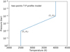 |
Fig. 1. Illustration of the two-point T–P profile assumption. |
To calculate a model spectrum of WASP-189b, we set the two points as (4000 K, 10−4 bar) and (2500 K, 10−2 bar) (shown in Fig. 1). We assumed a solar metallicity and set the volume mixing ratio of Fe I as a constant (10−4.59). Other parameters including the surface gravity and the stellar and planetary radii (Rp and Rs) are fixed to the values in Anderson et al. (2018). We neglected H− in the model calculation because adding H− only slightly changes the Fe I line depth (Fig. B.3). Rayleigh scattering is also not included in the model. After obtaining the thermal emission spectrum of the planet (Fp) with petitRADTRANS, we divided it by the blackbody spectrum of the star (Fs) to get the model spectrum 1 + Fp/Fs. This spectrum was then normalised by dividing it with the continuum spectrum 1 + Cp/Fs, where Cp is the blackbody spectrum of T2. The spectrum was subsequently convolved with the instrumental profile using the broadGaussFast code from the PyAstronomy library (Czesla et al. 2019). Figure 2 shows the final model spectrum, in which the Fe I lines have emission line shapes because the assumed T–P profile has a temperature inversion.
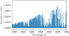 |
Fig. 2. Modelled thermal emission spectrum of Fe I. We assumed the T–P profile as in Fig. 1. The spectrum has been convolved to the resolution of the HARPS-N spectrograph and normalised. This model spectrum is used for cross-correlation. |
3.2. Cross-correlation with the Fe ı model
To search for the Fe I features in the dayside spectrum, we cross-correlated the observed data (i.e. the residual spectra after SYSREM procedures) with a grid of the model spectrum. The grid was established by shifting the model spectrum from –500 km s−1 to +500 km s−1 in 1 km s−1 steps. Here, we did not divide the data by the standard deviation because this procedure would modify the strength of the planetary signal (Brogi & Line 2019). Before the cross-correlation, we filtered the observed residual spectra using a Gaussian high-pass filter with a standard deviation of 15 points (∼9 km s−1) to remove any remaining broad-band features. For each of the residual spectra, we obtained a cross-correlation function (CCF):
 (2)
(2)
where ri is the residual spectra and mi is the shifted model spectrum at wavelength point i. We used the full wavelength coverage of the spectrograph excluding the O2 band at around 690 nm and the Na doublet line cores that are affected by interstellar medium absorption.
3.3. Cross-correlation results
The CCFs of all the observed spectra are presented in Fig. 3. The upper panel of Fig. 3 is the CCF-map in the stellar rest frame (i.e. with BERV and RVsys corrected). The planetary signal, which is the bright stripe with positive radial velocity (RV) before the eclipse and negative RV after the eclipse, is directly observable on the CCF-map. We established a model to fit the planetary RV signature directly on the CCF map. We assumed that the CCF has a Gaussian profile and the centre of the Gaussian profile is determined by the planetary velocity:
 (3)
(3)
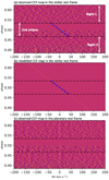 |
Fig. 3. Cross-correlation functions of the observations from the two nights. Upper and middle panels: observed and modelled CCF map in the stellar rest frame, respectively. The atmospheric Fe I signal is the bright stripe that appears during out-of-eclipse. The blue dashed lines indicate the expected planetary RV during eclipse. Bottom panel: CCF map with the planetary velocity (vp) corrected using the best-fit Kp and Δv values, and the atmospheric signal is the vertical stripe located around zero RV. |
where Kp is the semi-amplitude of the planetary orbital RV, ϕ is the orbital phase (ϕ = 0 is the mid-transit) and Δv is a RV deviation from the planetary orbital velocity. A circular orbit was adopted in the model. We then applied the Markov chain Monte Carlo (MCMC) simulations with the emcee tool (Foreman-Mackey et al. 2013) to fit the planetary signal on the CCF map. For each of the CCFs, we assigned its standard deviation as the noise. The best-fit result is  km s−1 for Kp and
  km s−1 for Δv. The obtained Kp is consistent with the expected Kp (
 km s−1) derived using Kepler’s third law with the orbital parameters from Anderson et al. (2018). The small Δv value could originate from several different sources, including the planetary atmospheric motion due to winds or rotation (Zhang et al. 2017; Flowers et al. 2019), the deviation of the absolute stellar RV relative to the measured RVsys (Yan et al. 2019), the uncertainty in the transit ephemeris (e.g. according to the orbital parameters in Anderson et al. (2018), the mid-transit time during our observations has an uncertainty of ∼300 s, which corresponds to a RV offset of 1.6 km s−1 at phases close to the secondary eclipse), and the eccentricity of the orbit. The lower panel of Fig. 3 presents the CCF map in the planetary rest frame and the atmospheric signal is the vertical bright stripe located around zero RV, as expected for a planetary signal.
We also generated the classical Kp-map by calculating the combined CCF for different Kp values (Fig. 4). The Kp-map is divided by the standard deviation of the region with |Δv| ranging from 100 to 200 km s−1. In this way, the value on the Kp-map represents the S/N. The Night-1 map has a stronger signal than the Night-2 map because the first half of the Night-2 data have lower S/Ns probably caused by a telescope focusing problem. The bottom panel presents the combined CCF of the data from the two nights at Kp = 193.5 km s−1, showing a detection of Fe I at S/N ∼ 8.7. The map generated using the data of both nights (Fig. 4c) has a very clear peak, demonstrating that Kp and Δv can be well constrained when combining the data observed before and after eclipse.
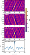 |
Fig. 4. The Kp–Δv maps. Panels a and b: maps for the Night-1 and Night-2 data, respectively. Panel c: map for the data from both nights combined. Bottom panel: CCF at the best-fit Kp. The dashed lines indicate the best-fit Kp and Δv values. |
The strong cross-correlation signal between the observed spectrum and the Fe I modelled emission spectrum indicates that the planetary Fe I lines have emission line profiles. Therefore, the detection is clear evidence of the existence of a strong temperature inversion layer in the planetary atmosphere. This result agrees with the theoretical simulation in Lothringer & Barman (2019), which suggests that UHJ can have a temperature inversion originating from atomic absorptions.
We also searched for other atomic species including Fe II, TiI, and Ti II using a similar method to that described above (i.e. cross-correlating the observed residual spectrum with the model spectrum assuming a two-point T–P profile and constant mixing ratios). We were not able to detect other atomic species. However, considering that Fe I has more lines than other atomic species, the non-detection does not mean that these species do not exist in the atmosphere. As we are detecting the thermal emission spectrum, other species may exist below or above the temperature inversion where the temperature could be close to isothermal, meaning that these species do not contribute to the emission spectrum. In addition, we searched for TiO and VO using the cross-correlation method, and did not detect any signal.
4. Retrieval of the temperature–pressure profile
4.1. Retrieval method
Although the cross-correlation results demonstrate the existence of a temperature inversion, the detailed T–P profile is not constrained. Retrieval methods for high-resolution spectroscopy have been developed in recent years (e.g. Brogi et al. 2017; Brogi & Line 2019; Shulyak et al. 2019; Fisher et al. 2020; Gibson et al. 2020). Following these works, we established a framework to retrieve the T–P profile of WASP-189b.
Since the Kp and the Δv are well determined by the cross-correlation method, we fixed these two values and shifted all the residual spectra to the planetary rest frame. We subsequently calculated a master residual spectrum (Ri) by averaging all the shifted spectra with their mean (S/N)2 as weight (Fig. B.1), excluding the ones taken in occultation. Following the method in Gibson et al. (2020), we assumed a standard Gaussian likelihood function and expressed it in logarithm as
![Mathematical equation: $$ \begin{aligned} \mathrm{ln} (L) = -\frac{1}{2}\sum _{i} \left[ \frac{(R_i - m_i)^2}{(\beta \sigma _i)^2} + \mathrm{ln} (2 \pi (\beta \sigma _i)^2) \right] , \end{aligned} $$](/articles/aa/full_html/2020/08/aa38294-20/aa38294-20-eq9.gif) (4)
(4)
where σi is the uncertainty of the observed residual spectrum Ri at wavelength point i and β is a scaling term of the uncertainty.
The model spectrum mi is calculated in a similar way as in Sect. 3.1.1. We assumed a two-points T–P profile and set T1, P1, T2, P2 and β as free parameters. We used uniform priors with boundaries shown in Table 2. In the retrieval work, the atmosphere consists of 81 layers uniformly spaced in log(P), with a pressure range of 10−8 bar – 1 bar. The volume mixing ratio of Fe I at each layer is calculated using the chemical module in the petitCode (Mollière et al. 2015, 2017), assuming a solar metallicity and equilibrium chemistry. The model takes into account thermal ionisation and condensation of Fe. Photochemistry is currently not included. According to the simulations of KELT-9b in Kitzmann et al. (2018), the effect of photochemistry on the Fe I mixing ratio is relatively weak and is negligible at pressures larger than 10−4 bar. Therefore, neglecting photochemistry only has a very limited effect on the retrieval. In addition to the Fe I lines, we also included Fe II in the model to make the retrieval more complete, although the contribution of the Fe II lines to the retrieved result is trivial. The model spectrum is convolved with the instrumental profile and normalised. We performed the retrieval with the MCMC tool emcee.
Best-fit parameters from the T–P profile retrieval.
4.2. Retrieval results and discussions
The best-fit T–P profile is presented in Fig. 5 together with a suite of profiles sampled by our analysis. The atmospheric parameters of the best fit are listed in Table 2 and the posterior distributions are shown in Fig. B.5. The retrieved β parameter has a value close to 1, indicating a proper error estimation in our analysis. The retrieved T–P profile indicates that the top of the stratosphere is located at ∼10−3.1 bar with a temperature of  K and the bottom of the stratosphere is located at ∼10−1.7 bar with a temperature of
  K. The contribution functions, which are defined as the fraction of flux a layer contributes to the total flux at given wavelengths, are shown in Fig. B.4. According to the contribution functions, the fluxes of the Fe I emission lines mostly originate from the upper layer of the inversion, and therefore the bottom of the inversion layer is less well confined. In the wavelength range of HARPS-N, the flux at the line core is determined by T1 and is much larger than the flux of the adjacent continuum that is determined by the blackbody spectrum at T2 (cf. Fig. B.2). Therefore, the lower boundary of T2 cannot be well determined as shown in the posterior distribution plot (Fig. B.5). There are other factors that can potentially affect the retrieved values, including uncertainties on the stellar and planetary parameters (e.g. Rp/Rs) as well as the assumed atmospheric metallicity.
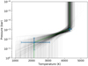 |
Fig. 5. Best-fit T–P profile retrieved from the Fe I emission lines (the blue points and the green line). The grey lines show random examples of T–P profile sampled by the MCMC analysis. The result is for the retrieval assuming solar metallicity. |
In the above retrieval work, we assumed the Fe metallicity ([Fe/H]) to be solar, but the retrieved T–P profile is related to the assumed [Fe/H]. We performed additional retrievals with [Fe/H] = −1 (i.e. decreasing the Fe metallicity tenfold) and [Fe/H] = +1 (i.e. increasing the Fe metallicity tenfold). The retrieved results are presented in Table 2. The T1 and T2 values remain similar when changing the Fe metallicity, while the P1 and P2 values vary with [Fe/H]. The Fe metallicity is actually degenerate with the pressures. This is because the strength of the Fe I emission lines are determined by the number density of Fe I at the upper layer of the inversion. Therefore, when assuming a higher metallicity, the retrieved P1 value is smaller, resulting in a similar Fe I number density around (T1, P1). Detecting other chemical species (e.g. FeH and CO) in the near-infrared will probably allow the degeneracy to be broken and the atmospheric metallicity to be constrained.
The retrieved T–P profile is consistent with the prediction by Lothringer & Barman (2019) of strong temperature inversions in the atmospheres of UHJs orbiting early-type stars. WASP-189b orbits around an A6-type star and has a very hot dayside atmosphere that is probably dominated by atomic species such as Fe I. Since the planet receives a large amount of optical and UV irradiation, the absorption of the stellar flux by these atomic species can heat the atmosphere and produce the temperature inversion observed in this work. Although our result indicates the inversion could be created by absorptions of atomic species like Fe I, a comprehensive self-consistent radiation transfer model is required to calculate the actual opacity contributions in the inversion layer.
The strong and dense Fe I emission lines in the optical wavelengths also increase the overall flux level of the planetary dayside (cf. Fig. B.2). Therefore, when measuring the secondary eclipse in photometry, the obtained eclipse depth will probably be larger than the depth corresponding to the planetary equilibrium temperature.
5. Conclusions
We observed the dayside thermal emission spectrum of WASP-189b with the HARPS-N spectrograph. Utilising the cross-correlation technique, we detected a strong signal of Fe I lines in emission line shapes, which is direct evidence of a temperature inversion. We fitted the observed Fe I spectrum with theoretical models assuming a two-point temperature–pressure profile. The retrieved T–P profile has a temperature inversion layer located between ∼10−1.7 bar and ∼10−3.1 bar when assuming a solar metallicity, and the top of the inversion layer has a very hot temperature of  K. We also searched for other species (including Fe II, Ti I, Ti II, and TiO/VO) and were not able to detect them. The non-detection could be attributed to either the lack of sufficient lines in the HARPS-N wavelengths or the non-existence of these species in the temperature inversion layer of the planetary atmosphere.
Several UHJs have temperature inversions detected in their dayside atmospheres, although the formation of the inversion is still under debate. Our detection of a temperature inversion with atomic iron in WASP-189b indicates that temperature inversions in UHJs are probably partially or completed produced by atomic absorptions of the stellar optical and UV irradiation. However, TiO/VO or other metal compounds could still contribute to the formation of temperature inversion. Further observations at multiple wavelengths and both low and high spectral resolutions will allow us to decipher comprehensive chemical and temperature structures for these planets. Expanding the observations to other UHJs will allow us to explore the diversity of temperature structures related to different chemical species and host star types.
Acknowledgments
We thank the referee for his/her useful comments. F.Y. acknowledges the support of the DFG priority program SPP 1992 “Exploring the Diversity of Extrasolar Planets (RE 1664/16-1)”. This work is based on observations made with the Italian Telescopio Nazionale Galileo (TNG) operated on the island of La Palma by the Fundación Galileo Galilei of the INAF (Istituto Nazionale di Astrofisica) at the Spanish Observatorio del Roque de los Muchachos of the Instituto de Astrofisica de Canarias. This work is partly financed by the Spanish Ministry of Economics and Competitiveness through project ESP2016-80435-C2-2-R and PGC2018-098153-B-C31. G.C. acknowledges the support by the Natural Science Foundation of Jiangsu Province (Grant No. BK20190110). P.M. acknowledges support from the European Research Council under the European Union’s Horizon 2020 research and innovation program under grant agreement No. 832428.
References
- Anderson, D. R., Temple, L. Y., & Nielsen, L. D. 2018, MNRAS, submitted [arXiv:1809.04897] [Google Scholar]
- Arcangeli, J., Désert, J.-M., Line, M. R., et al. 2018, ApJ, 855, L30 [NASA ADS] [CrossRef] [Google Scholar]
- Ben-Yami, M., Madhusudhan, N., Cabot, S. H. C., et al. 2020, ApJ, 897, L5 [CrossRef] [Google Scholar]
- Berdiñas, Z. M., Amado, P. J., Anglada-Escudé, G., Rodríguez-López, C., & Barnes, J. 2016, MNRAS, 459, 3551 [NASA ADS] [CrossRef] [Google Scholar]
- Birkby, J. L., de Kok, R. J., Brogi, M., et al. 2013, MNRAS, 436, L35 [NASA ADS] [CrossRef] [Google Scholar]
- Birkby, J. L., de Kok, R. J., Brogi, M., Schwarz, H., & Snellen, I. A. G. 2017, AJ, 153, 138 [NASA ADS] [CrossRef] [Google Scholar]
- Brogi, M., & Line, M. R. 2019, AJ, 157, 114 [NASA ADS] [CrossRef] [Google Scholar]
- Brogi, M., Snellen, I. A. G., de Kok, R. J., et al. 2012, Nature, 486, 502 [NASA ADS] [CrossRef] [PubMed] [Google Scholar]
- Brogi, M., de Kok, R. J., Birkby, J. L., Schwarz, H., & Snellen, I. A. G. 2014, A&A, 565, A124 [NASA ADS] [CrossRef] [EDP Sciences] [Google Scholar]
- Brogi, M., Line, M., Bean, J., Désert, J. M., & Schwarz, H. 2017, ApJ, 839, L2 [NASA ADS] [CrossRef] [Google Scholar]
- Casasayas-Barris, N., Pallé, E., Yan, F., et al. 2018, A&A, 616, A151 [NASA ADS] [CrossRef] [EDP Sciences] [Google Scholar]
- Casasayas-Barris, N., Pallé, E., Yan, F., et al. 2019, A&A, 628, A9 [NASA ADS] [CrossRef] [EDP Sciences] [Google Scholar]
- Cauley, P. W., Shkolnik, E. L., Ilyin, I., et al. 2019, AJ, 157, 69 [NASA ADS] [CrossRef] [Google Scholar]
- Cauley, P. W., Shkolnik, E. L., Ilyin, I., et al. 2020, Res. Notes Am. Astron. Soc., 4, 53 [Google Scholar]
- Charbonneau, D., Knutson, H. A., Barman, T., et al. 2008, ApJ, 686, 1341 [NASA ADS] [CrossRef] [MathSciNet] [Google Scholar]
- Czesla, S., Schröter, S., & Schneider, C. P. 2019, PyA: Python Astronomy-related Packages, Astrophysics Source Code Library [record ascl:1906.010] [Google Scholar]
- Désert, J. M., Vidal-Madjar, A., & Lecavelier Des Etangs, A. 2008, A&A, 492, 585 [NASA ADS] [CrossRef] [EDP Sciences] [Google Scholar]
- Diamond-Lowe, H., Stevenson, K. B., Bean, J. L., Line, M. R., & Fortney, J. J. 2014, ApJ, 796, 66 [NASA ADS] [CrossRef] [Google Scholar]
- Ehrenreich, D., Lovis, C., & Allart, R. 2020, Nature, 580, 567 [Google Scholar]
- Espinoza, N., Rackham, B. V., Jordán, A., et al. 2019, MNRAS, 482, 2065 [Google Scholar]
- Evans, T. M., Sing, D. K., Kataria, T., et al. 2017, Nature, 548, 58 [NASA ADS] [CrossRef] [Google Scholar]
- Fisher, C., Hoeijmakers, H. J., Kitzmann, D., et al. 2020, AJ, 159, 192 [CrossRef] [Google Scholar]
- Flowers, E., Brogi, M., Rauscher, E., Kempton, E. M. R., & Chiavassa, A. 2019, AJ, 157, 209 [NASA ADS] [CrossRef] [Google Scholar]
- Foreman-Mackey, D., Hogg, D. W., Lang, D., & Goodman, J. 2013, PASP, 125, 306 [CrossRef] [Google Scholar]
- Fortney, J. J., Lodders, K., Marley, M. S., & Freedman, R. S. 2008, ApJ, 678, 1419 [NASA ADS] [CrossRef] [Google Scholar]
- Gibson, N. P., Merritt, S., Nugroho, S. K., et al. 2020, MNRAS, 493, 2215 [NASA ADS] [CrossRef] [Google Scholar]
- Haynes, K., Mandell, A. M., Madhusudhan, N., Deming, D., & Knutson, H. 2015, ApJ, 806, 146 [NASA ADS] [CrossRef] [Google Scholar]
- Helling, C., Gourbin, P., Woitke, P., & Parmentier, V. 2019, A&A, 626, A133 [CrossRef] [Google Scholar]
- Hoeijmakers, H. J., Ehrenreich, D., Heng, K., et al. 2018, Nature, 560, 453 [NASA ADS] [CrossRef] [Google Scholar]
- Hoeijmakers, H. J., Ehrenreich, D., Kitzmann, D., et al. 2019, A&A, 627, A165 [NASA ADS] [CrossRef] [EDP Sciences] [Google Scholar]
- Hoeijmakers, H. J., Cabot, S. H. C., & Zhao, L. 2020a, A&A, in press, https://doi.org/10.1051/0004-6361/202037437 [Google Scholar]
- Hoeijmakers, H. J., Seidel, J. V., & Pino, L. 2020b, A&A, accepted [arXiv:2006.11308] [Google Scholar]
- Hubeny, I., Burrows, A., & Sudarsky, D. 2003, ApJ, 594, 1011 [NASA ADS] [CrossRef] [Google Scholar]
- Jensen, A. G., Cauley, P. W., Redfield, S., Cochran, W. D., & Endl, M. 2018, AJ, 156, 154 [NASA ADS] [CrossRef] [Google Scholar]
- Kitzmann, D., Heng, K., Rimmer, P. B., et al. 2018, ApJ, 863, 183 [NASA ADS] [CrossRef] [Google Scholar]
- Knutson, H. A., Charbonneau, D., Allen, L. E., Burrows, A., & Megeath, S. T. 2008, ApJ, 673, 526 [NASA ADS] [CrossRef] [Google Scholar]
- Kreidberg, L., Line, M. R., Parmentier, V., et al. 2018, AJ, 156, 17 [NASA ADS] [CrossRef] [Google Scholar]
- Line, M. R., Stevenson, K. B., Bean, J., et al. 2016, AJ, 152, 203 [NASA ADS] [CrossRef] [Google Scholar]
- Lothringer, J. D., & Barman, T. 2019, ApJ, 876, 69 [NASA ADS] [CrossRef] [Google Scholar]
- Lothringer, J. D., Barman, T., & Koskinen, T. 2018, ApJ, 866, 27 [NASA ADS] [CrossRef] [Google Scholar]
- Merritt, S. R., Gibson, N. P., Nugroho, S. K., et al. 2020, A&A, 636, A117 [CrossRef] [EDP Sciences] [Google Scholar]
- Mollière, P., van Boekel, R., Dullemond, C., Henning, T., & Mordasini, C. 2015, ApJ, 813, 47 [NASA ADS] [CrossRef] [Google Scholar]
- Mollière, P., van Boekel, R., Bouwman, J., et al. 2017, A&A, 600, A10 [NASA ADS] [CrossRef] [EDP Sciences] [Google Scholar]
- Mollière, P., Wardenier, J. P., van Boekel, R., et al. 2019, A&A, 627, A67 [NASA ADS] [CrossRef] [EDP Sciences] [Google Scholar]
- Nugroho, S. K., Kawahara, H., Masuda, K., et al. 2017, AJ, 154, 221 [NASA ADS] [CrossRef] [Google Scholar]
- Nugroho, S. K., Gibson, N. P., de Mooij, E. J. W., et al. 2020, MNRAS, 496, 504 [CrossRef] [Google Scholar]
- O’Donovan, F. T., Charbonneau, D., Harrington, J., et al. 2010, ApJ, 710, 1551 [NASA ADS] [CrossRef] [Google Scholar]
- Parmentier, V., Line, M. R., Bean, J. L., et al. 2018, A&A, 617, A110 [NASA ADS] [CrossRef] [EDP Sciences] [Google Scholar]
- Pino, L., Désert, J.-M., Brogi, M., et al. 2020, ApJ, 894, L27 [NASA ADS] [CrossRef] [Google Scholar]
- Schwarz, H., Brogi, M., de Kok, R., Birkby, J., & Snellen, I. 2015, A&A, 576, A111 [NASA ADS] [CrossRef] [EDP Sciences] [Google Scholar]
- Sedaghati, E., Boffin, H. M. J., MacDonald, R. J., et al. 2017, Nature, 549, 238 [NASA ADS] [CrossRef] [Google Scholar]
- Sheppard, K. B., Mandell, A. M., Tamburo, P., et al. 2017, ApJ, 850, L32 [NASA ADS] [CrossRef] [Google Scholar]
- Shulyak, D., Rengel, M., Reiners, A., Seemann, U., & Yan, F. 2019, A&A, 629, A109 [CrossRef] [EDP Sciences] [Google Scholar]
- Sing, D. K., Lavvas, P., Ballester, G. E., et al. 2019, AJ, 158, 91 [NASA ADS] [CrossRef] [Google Scholar]
- Snellen, I. A. G., de Kok, R. J., de Mooij, E. J. W., & Albrecht, S. 2010, Nature, 465, 1049 [NASA ADS] [CrossRef] [PubMed] [Google Scholar]
- Snellen, I. A. G., Brandl, B. R., de Kok, R. J., et al. 2014, Nature, 509, 63 [NASA ADS] [CrossRef] [Google Scholar]
- Stangret, M., Casasayas-Barris, N., Pallé, E., et al. 2020, A&A, 638, A26 [CrossRef] [EDP Sciences] [Google Scholar]
- Tamuz, O., Mazeh, T., & Zucker, S. 2005, MNRAS, 356, 1466 [NASA ADS] [CrossRef] [Google Scholar]
- Todorov, K., Deming, D., Harrington, J., et al. 2010, ApJ, 708, 498 [NASA ADS] [CrossRef] [Google Scholar]
- Turner, J. D., de Mooij, E. J. W., Jayawardhana, R., et al. 2020, ApJ, 888, L13 [NASA ADS] [CrossRef] [Google Scholar]
- Yan, F., & Henning, T. 2018, Nat. Astron., 2, 714 [NASA ADS] [CrossRef] [Google Scholar]
- Yan, F., Casasayas-Barris, N., Molaverdikhani, K., et al. 2019, A&A, 632, A69 [NASA ADS] [CrossRef] [EDP Sciences] [Google Scholar]
- Zellem, R. T., Lewis, N. K., Knutson, H. A., et al. 2014, ApJ, 790, 53 [NASA ADS] [CrossRef] [EDP Sciences] [Google Scholar]
- Zhang, J., Kempton, E. M. R., & Rauscher, E. 2017, ApJ, 851, 84 [CrossRef] [Google Scholar]
Appendix A: Removal of stellar and telluric lines with SYSREM
The SYSREM algorithm (Tamuz et al. 2005) has been demonstrated to be a robust technique to remove the stellar and telluric lines for high-resolution spectroscopy (Birkby et al. 2013; Snellen et al. 2014; Birkby et al. 2017). The input data for the SYSREM algorithm is the normalised and blaze-variation-corrected spectral matrix. We chose a SYSREM iteration of 6 because the S/Ns of the planetary signal are relatively high for both nights at this iteration. We tested different iterations and found that the results do not change significantly.
In order to preserve the relative depths of the planetary lines, we used the same method as in Gibson et al. (2020). Firstly, we applied the SYSREM iterations in the classical way. Subsequently, instead of using the subtracting residual as the final product, we summed the SYSREM models from each iteration and divided the original input data by the final model. In this way, the strengths of the planetary signals located at the stellar and telluric absorption lines are preserved and the residual spectra represent the normalised spectra of 1 + Fp/Fs. We performed the SYSREM with data in flux-space, while the SYSREM method was originally used for data in magnitude-space (Tamuz et al. 2005). We note that dividing the SYSREM models in flux-space as described above is mostly equivalent to subtracting the SYSREM models in magnitude-space.
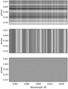 |
Fig. A.1. Example of the data-reduction procedures. These data are from Night-1 observation. (a) original spectra from the HARPS-N pipeline (Data Reduction Software). These are order-merged spectra. Here the spectra are shifted into the Earth’s rest frame. (b) spectra after normalisation and correction of blaze variations. (c) residual spectra after the removal of stellar and telluric lines using SYSREM. |
Appendix B: Additional figures
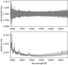 |
Fig. B.1. Upper panel: master residual spectrum. This is the combination of all the residual spectra of the two nights, excluding the spectra taken in eclipse. Lower panel: uncertainty of the master residual spectrum. |
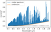 |
Fig. B.2. Example of the modelled spectrum (the blue line) and the corresponding continuum (the orange line). The dashed black line shows the zero flux level. The spectra were calculated using the best-fit T–P profile in Fig. 5. The continuum corresponds to the blackbody spectrum at the temperature of T2. In the HARPS-N wavelength range (i.e. below 0.69 μm), the flux at the Fe I line core is much larger than the continuum flux. |
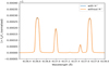 |
Fig. B.3. Comparison between the normalised model spectra with and without the H− continuum opacity. The spectra were calculated using the same parameters as in Fig. B.2. The line depths between the two models are almost the same, indicating that the H− contribution can be neglected in our analysis. |
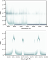 |
Fig. B.4. Contribution functions of the thermal emission spectrum calculated using the same parameters as in Fig. B.2. Upper panel: presents the contribution functions over the entire HARPS-N wavelength range and Bottom panel: detailed view in a narrow wavelength range. The contribution functions indicate that the fluxes of the Fe lines are from the upper layer of the temperature inversion, while the continuum flux is from the low altitudes. It appears that we are probing the continuum at the bottom of the atmosphere (which is set as 1 bar), but this result is due to the model setup (i.e. isothermal for pressures larger than P2). The continuum spectrum is the same if we set the atmospheric lower boundary at P2 instead of 1 bar. |
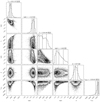 |
Fig. B.5. Posterior distribution of the parameters from the MCMC fit. Tslope is not a fitted parameter, but is calculated using Eq. (1). |
All Tables
All Figures
|
Fig. 1. Illustration of the two-point T–P profile assumption. |
| In the text | |
|
Fig. 2. Modelled thermal emission spectrum of Fe I. We assumed the T–P profile as in Fig. 1. The spectrum has been convolved to the resolution of the HARPS-N spectrograph and normalised. This model spectrum is used for cross-correlation. |
| In the text | |
|
Fig. 3. Cross-correlation functions of the observations from the two nights. Upper and middle panels: observed and modelled CCF map in the stellar rest frame, respectively. The atmospheric Fe I signal is the bright stripe that appears during out-of-eclipse. The blue dashed lines indicate the expected planetary RV during eclipse. Bottom panel: CCF map with the planetary velocity (vp) corrected using the best-fit Kp and Δv values, and the atmospheric signal is the vertical stripe located around zero RV. |
| In the text | |
|
Fig. 4. The Kp–Δv maps. Panels a and b: maps for the Night-1 and Night-2 data, respectively. Panel c: map for the data from both nights combined. Bottom panel: CCF at the best-fit Kp. The dashed lines indicate the best-fit Kp and Δv values. |
| In the text | |
|
Fig. 5. Best-fit T–P profile retrieved from the Fe I emission lines (the blue points and the green line). The grey lines show random examples of T–P profile sampled by the MCMC analysis. The result is for the retrieval assuming solar metallicity. |
| In the text | |
|
Fig. A.1. Example of the data-reduction procedures. These data are from Night-1 observation. (a) original spectra from the HARPS-N pipeline (Data Reduction Software). These are order-merged spectra. Here the spectra are shifted into the Earth’s rest frame. (b) spectra after normalisation and correction of blaze variations. (c) residual spectra after the removal of stellar and telluric lines using SYSREM. |
| In the text | |
|
Fig. B.1. Upper panel: master residual spectrum. This is the combination of all the residual spectra of the two nights, excluding the spectra taken in eclipse. Lower panel: uncertainty of the master residual spectrum. |
| In the text | |
|
Fig. B.2. Example of the modelled spectrum (the blue line) and the corresponding continuum (the orange line). The dashed black line shows the zero flux level. The spectra were calculated using the best-fit T–P profile in Fig. 5. The continuum corresponds to the blackbody spectrum at the temperature of T2. In the HARPS-N wavelength range (i.e. below 0.69 μm), the flux at the Fe I line core is much larger than the continuum flux. |
| In the text | |
|
Fig. B.3. Comparison between the normalised model spectra with and without the H− continuum opacity. The spectra were calculated using the same parameters as in Fig. B.2. The line depths between the two models are almost the same, indicating that the H− contribution can be neglected in our analysis. |
| In the text | |
|
Fig. B.4. Contribution functions of the thermal emission spectrum calculated using the same parameters as in Fig. B.2. Upper panel: presents the contribution functions over the entire HARPS-N wavelength range and Bottom panel: detailed view in a narrow wavelength range. The contribution functions indicate that the fluxes of the Fe lines are from the upper layer of the temperature inversion, while the continuum flux is from the low altitudes. It appears that we are probing the continuum at the bottom of the atmosphere (which is set as 1 bar), but this result is due to the model setup (i.e. isothermal for pressures larger than P2). The continuum spectrum is the same if we set the atmospheric lower boundary at P2 instead of 1 bar. |
| In the text | |
|
Fig. B.5. Posterior distribution of the parameters from the MCMC fit. Tslope is not a fitted parameter, but is calculated using Eq. (1). |
| In the text | |
Current usage metrics show cumulative count of Article Views (full-text article views including HTML views, PDF and ePub downloads, according to the available data) and Abstracts Views on Vision4Press platform.
Data correspond to usage on the plateform after 2015. The current usage metrics is available 48-96 hours after online publication and is updated daily on week days.
Initial download of the metrics may take a while.