| Issue |
A&A
Volume 640, August 2020
|
|
|---|---|---|
| Article Number | A38 | |
| Number of page(s) | 28 | |
| Section | Extragalactic astronomy | |
| DOI | https://doi.org/10.1051/0004-6361/202038156 | |
| Published online | 10 August 2020 | |
Morphology and surface photometry of a sample of isolated early-type galaxies from deep imaging⋆
1
INAF Osservatorio Astronomico di Padova, Via dell’Osservatorio 8, 36012 Asiago, Italy
e-mail: This email address is being protected from spambots. You need JavaScript enabled to view it.
2
Vatican Observatory, Vatican City
e-mail: This email address is being protected from spambots. You need JavaScript enabled to view it.
3
INAF-IASF, Via A. Curti 12, 20133 Milano, Italy
e-mail: This email address is being protected from spambots. You need JavaScript enabled to view it.
4
Dep.to Astronomia Extragaláctica Istituto Astrofisica de Andalucía, Glorieta de la Astronomia s/n, 18008 Granada, Spain
5
INAF Osservatorio Astronomico di Padova, Vicolo dell’Osservatorio 5, 35122 Padova, Italy
Received:
13
April
2020
Accepted:
22
May
2020
Abstract
Context. Isolated early-type galaxies are evolving in unusually poor environments for this morphological family, which is typical of cluster inhabitants. We investigate the mechanisms driving the evolution of these galaxies.
Aims. Several studies indicate that interactions, accretions, and merging episodes leave their signature on the galaxy structure, from the nucleus down to the faint outskirts. We focus on revealing such signatures, if any, in a sample of isolated early-type galaxies, and we quantitatively revise their galaxy classification.
Methods. We observed 20 (out of 104) isolated early-type galaxies, selected from the AMIGA catalog, with the 4KCCD camera at the Vatican Advanced Technology Telescope in the Sloan Digital Sky Survey g and r bands. These are the deepest observations of a sample of isolated early-type galaxies so far: on average, the light profiles reach μg ≈ 28.11 ± 0.70 mag arcsec−2 and μr ≈ 27.36 ± 0.68 mag arcsec−2. The analysis was performed using the AIDA package, providing point spread function-corrected 2D surface photometry up to the galaxy outskirts. The package provides a model of the 2D galaxy light distribution, which after model subtraction enhances the fine and peculiar structures in the residual image of the galaxies.
Results. Our re-classification suggests that the sample is composed of bona fide early-type galaxies spanning from ellipticals to late-S0s galaxies. Most of the surface brightness profiles are best fitted with a bulge plus disc model, suggesting the presence of an underlying disc structure. The residuals obtained after the model subtraction show the nearly ubiquitous presence of fine structures, such as shells, stellar fans, rings, and tails. Shell systems are revealed in about 60% of these galaxies.
Conclusions. Because interaction, accretion, and merging events are widely interpreted as the origin of the fans, ripples, shells and tails in galaxies, we suggest that most of these isolated early-type galaxies have experienced such events. Because they are isolated (after 2–3 Gyr), these galaxies are the cleanest environment in which to study phenomena connected with events like these.
Key words: galaxies: elliptical and lenticular, cD / galaxies: photometry / galaxies: interaction / galaxies: evolution
The reduced images are only available at the CDS via anonymous ftp to cdsarc.u-strasbg.fr (130.79.128.5) or via http://cdsarc.u-strasbg.fr/viz-bin/cat/J/A+A/640/A38
© ESO 2020
1. Introduction
Since the discovery of the morphology-density relation, early-type galaxies (Es + S0s = ETGs hereafter) have been known to be typical inhabitants of dense clusters (Dressler 1980; Houghton 2015). Although with the large uncertainty introduced by automatic galaxy classifications, studies based on the Sloan Digital Sky Survey (SDSS; see e.g. York 2000; Abazajian et al. 2009) have shown that ETGs represent a minority (≈10% E and ≈20% S0s) of the galaxy population in the lowest density fields (see e.g. Goto et al. 2003, their Fig. 12). One of the pioneering attempts to characterise the population of galaxies in relatively high isolation produced the Catalog of Isolated Galaxies in the Northern Hemisphere by Karachentseva (1973), which includes a small set of isolated ETGs (iETGs hereafter). Several catalogues of isolated galaxies have been produced since then (e.g. Verdes-Montenegro et al. 2005; Hernández-Toledo et al. 2010; Argudo-Fernàndez et al. 2013, 2015). Historically, these efforts are intended to provide the best sample of unperturbed galaxies to be used as a baseline for comparison of galaxy properties with interacting or cluster samples, for example (see e.g. Rampazzo 2016).
The study of the evolutionary scenario that gives rise to iETGs is of particular interest because their environment is so unusual for this class of galaxy. ETGs are thought to be the final product of the galaxy evolution, where different phenomena, from secular to accretion driven, can play a role (Cappellari 2016). Simulations suggest that interaction, accretion and merging episodes (see Eliche-Moral et al. 2018; Mazzei et al. 2019, and references therein) leave their signatures on galaxies, from the nuclear cuspy versus core shape (Lauer et al. 1991, 1992; Lauer 2012; Côtè et al. 2006; Turner et al. 2012) to their outskirts, where tails, streams, fans, and shells may be found (Arp 1966; Malin & Carter 1983; Prieur 1988; Wilkinson et al. 2000; Duc et al. 2015). Shells are often found in ETGs. They are described as interleaved stellar tidal debris with large opening angles and low surface brightness that are often situated on either side of the galaxy centre and have regular as well as irregular shapes (Dupraz & Combes 1987; Weil & Hernquist 1993; Pop et al. 2018; Mancillas et al. 2019). These signatures have different lifetimes and originate from different mechanisms. Recently, Mancillas et al. (2019) pointed out that tails emerge from the primary galaxy and streams are generated from the secondary galaxy. Tails have shorter lifetimes (2 Gyr) than shells. Shells are generated by minor and major either wet or dry mergers and are long lasting (3 Gyr) (see also Dupraz & Combes 1987; Weil & Hernquist 1993; Longhetti et al. 1999). Streams remains visible in all phases of galaxy evolution.
For iETGs, the detection of these fine structures may help to understand the time that elapsed from their last interaction, accretion, and merging episode. In general, ETGs in low-density environments are found to be rejuvenated in their centre as well as in their outskirts, as shown by the Galaxy Evolution Explorer (GALEX; Martin et al. 2006), suggesting that some form of activity might be induced by interaction, accretion, and merging episodes (Clemens et al. 2006, 2009; Schawinski et al. 2007; Rampazzo et al. 2007; Marino et al. 2011a,b; Mazzei et al. 2014a,b, 2019; Mapelli et al. 2015; Hagen et al. 2016, and references therein).
The SDSS has widely contributed to the investigation of iETGs. Many studies have been dedicated to a visual re-classification of the galaxies in the Karachentseva (1973) catalog and/or revisions of it (Sulentic et al. 2006; Fernandez-Lorenzo et al. 2012; Buta et al. 2019). Hernández-Toledo et al. (2008; H-T hereafter) performed a study (using DR6) of the 579 galaxies in the Karachentseva (1973) sample, including iETGs (58 E, 14 E/S0, 67 S0, and 19 S0/a). They revised the ETG classification on the basis of the geometric profiles obtained by r-band images using IRAF (Jedrzejewski 1987). This process classified only 18 galaxies (3.5% of the entire sample) as bona fide E. They are listed in their Table 6. The authors report a 50% incidence of ripples and shells in these Es (9 out of 18), see Table 6 of the paper, although 4 are uncertain detections) as well as a high fraction of Es with diffuse halo (7 out of 18). Recently, Rampazzo et al. (2019) found interaction and merging signatures in a high spatial resolution study in K band, performed with ARGOS+LUCI at the Large Binocular Telescope (LBT; Rabien et al. 2019), of KIG 685 and KIG 895. This latter has been found to be a misclassified spiral with a tail. KIG 685 is a bona fide ETG with shells that would suggest an eventful life like that of ETGs in loose galaxy associations, where shells, for instance, are found with a higher frequency than in clusters (see e.g. Malin & Carter 1983; Reduzzi et al. 1996).
The above studies emphasised two aspects. The first aspect is the lack of a quantitative classification of the morphology of isolated galaxies, in particular, of iETGs whose classification is still very uncertain (cf. Sect. 2). For example, H-T found that E+S0 make up 8.5% (3.5% + 5%) of E + S0 + E/S0 (5.7% + 6.6% + 1.4%), while Sulentic et al. (2006) found them to make up 13.7%. The other aspect is that we need surface photometric studies that are deep enough to reveal the fine structure of iETGs, if any. These considerations motivated the present study. Using g and r deep surface photometry, we search for such faint features in iETGs and refine the previously proposed iETG galaxy morphological classification (Sulentic et al. 2006; Fernandez-Lorenzo et al. 2012; Buta et al. 2019) by substantiating the view of H-T about the rarity of Es versus S0s in samples of isolated galaxies. This will help understand their evolutionary mechanisms and the meaning of their current relative isolation.
The paper is structured as follows. The observed sample is presented in Sect. 2. In Sect. 3 we present the observations performed at the Vatican Advanced Technology Telescope (VATT) with the 4K CCD camera. This section also describes the reduction method we implement that fully exploits the quality of the observations. Results are presented in Sect. 4. In Sect. 5 we discuss our results to understand the nature and evolutionary paths of our iETGs.
2. The sample
The sample set is composed of 20 iETGs that are included in the Analysis of the interstellar Medium of Isolated Galaxies sample (AMIGA, Verdes-Montenegro et al. (2005)), which is a revision of the 1973 catalogue of Karachentseva (1973). The analysis of the AMIGA sample revealed a set of galaxies that should not have interacted for at least 3 Gyr (Verdes-Montenegro et al. 2005; Verley et al. 2007a,b).
2.1. The iETGs classification problem
In addition to the morphological classification, we selected the sample by considering the galaxy observability (see Sect. 3). We selected galaxies using the classification of Fernandez-Lorenzo et al. (2012), which is an updated version of the Sulentic et al. (2006) classification. For comparison, we also considered the classification provided by HyperLeda and the recent morphological classification by Buta et al. (2019). We collect in Table 1 and Table 2 the classifications and the main galaxy characteristics. In the results section (Sect. 4) we also consider the classification of H-T, which is based on the geometrical profiles of the galaxies.
Sample: KIGs morphology, heliocentric velocity, and adopted distance.
The differences among the classifications are summarised in Fig. 1. The morphological type distribution, provided by Fernandez-Lorenzo et al. (2012), ranges from −5 ≤ T ≤ 0, that is, it covers the entire range of iETGs, and contains a large portion of galaxies with a disc component (−3 < T < 0). However, we note that the galaxy morphological classification is often (largely) discordant among these authors, as shown in Table 1 and Fig. 1. Some galaxies, that is, KIG 481 and KIG 620, are late type (T > 0) according to Buta et al. (2019), and KIG 620, KIG 644, and KIG 733, which are all seen edge-on, are classified as late type by HyperLeda.
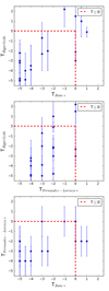 |
Fig. 1. Comparison between the three classifications into morphological type provided in Table 1. The dashed red rectangle encloses iETGs (T ≤ 0) in the RC3 classification. Comparisons are made between HyperLeda vs. Buta et al. (2019) (top panel), HyperLeda vs. Fernandez-Lorenzo et al. (2012) (middle panel), and Buta et al. (2019) vs. Fernandez-Lorenzo et al. (2012) (bottom panel). |
Buta et al. (2019), who most recently classified our iETGs visually, on average tend to provide earlier ΔT = −0.5 morphological type than both HyperLeda and Fernandez-Lorenzo et al. (2012). These latter classifications differ by ΔT = 0.05 on average, but single cases may differ more significantly, as shown in the middle panel of Fig. 1. We here quantitatively verify the classification using surface photometry, for example, by determining the presence of a disc. Out of 20 ETGs, 5 show peculiarities (pec) according to the Buta et al. (2019) classification: KIG 481, KIG 490, KIG 685, KIG 733, and KIG 841.
The heliocentric velocity of only two objects is lower than 3000 km s−1. These are KIG 481 and KIG 637. The average heliocentric velocity is Vhel = 8535 km s−1 (Table 1). Distances are taken from Jones et al. (2018), who analysed the AMIGA sample in H I. They used the Mould et al. (2000) model for distances. This model corrects for Local Group motion and uses separate attractor velocity fields for the Virgo cluster, the Shapley supercluster, and the Great Attractor. The distance is finally obtained by adopting H0 = 70 km s−1 Mpc−1. The relevant photometric properties of iETGs are collected in Table 2. The g and r photometric data sets are taken from the SLOAN (CModel) values reported in NED. The GALEX near-UV (NUV hereafter) integrated magnitudes are also taken from NED.
KIG relevant geometric and photometric properties.
2.2. Degree of isolation in the sample
The environment of the AMIGA galaxies was investigated to avoid similar size companions. Different criteria were developed to define the isolation parameters (Verley et al. 2007a; Argudo-Fernàndez et al. 2013, 2015). Fig. 2 shows the isolation parameters of the 114 iETGs in the AMIGA sample classified by Fernandez-Lorenzo et al. (2012), devised by Verley et al. (2007a). Verley et al. (2007a) calculated the ηK and QKar parameters by defining the local galaxy number density and the distribution of the tidal strength, respectively. According to the Verley et al. (2007a) parameters, the four galaxies KIG 412, KIG 595, KIG 644, and KIG 637 are located outside the fiducial range in the Q versus ηk plane for isolated galaxies (dashed horizontal and vertical lines in Fig. 2).
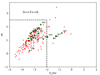 |
Fig. 2. Degree of isolation of the observed sample (green circles) over-plotted on all iETGs (red circles) in the AMIGA sample. According to Verley et al. (2007a), the horizontal and vertical dashed lines enclose the fiducial range of isolated galaxies in the AMIGA sample. |
More recently, Argudo-Fernàndez et al. (2013) further revised the isolation criteria of the AMIGA galaxies using both photometric and spectroscopic data from SDSS to refine the ηK and QKar parameters. Of the iETGs in this work, Argudo-Fernàndez et al. (2013) found that only KIG 599 is considered isolated when the original isolation criteria of Karachentseva (1973) are applied to SDSS images. However, most of the iETGs pass the criteria for the (photometric) tidal interaction and neighbour density parameters recommended by Argudo-Fernàndez et al. (2013), QKar < −2 and ηK < 2.7, meaning that they are assumed to be minimally affected by any neighbours. The exceptions are KIG 517, KIG 644, KIG 722, and KIG 733, all of which violate the neighbour density criterion, but not the tidal interaction criterion. In their spectroscopic analysis, Argudo-Fernàndez et al. (2013) found that about half of the iETG sample do fulfil the Karachentseva isolation criteria when neighbours separated by more than 500 km s−1 from the target (in redshift) are removed. This includes KIG 644 and KIG 733, which did not pass the photometric criteria. The galaxies that fail are KIG 264, KIG 517, KIG 595, KIG 620, KIG 637, and KIG 722. There are no measurements (photometric or spectroscopic) for KIG 481, KIG 670, or KIG 732, and KIG 841 lacks spectroscopic measurements. In the cases of KIG 412 and KIG 644, Argudo-Fernàndez et al. (2013) is at odds with Verley et al. (2007a) because they did not meet the previous criteria. When they used the spectroscopic data, Argudo-Fernàndez et al. (2013) found that approximately 70% of the AMIGA galaxies meet the Karachentseva criteria for isolation. For these iETGs, this number is 63 ± 10% (the error is due to galaxies without data). About half of the iETGs do not pass the strictest test, but are still expected to be only minimally affected by any neighbours (except possibly KIG 595, those with missing data, and the two conflicts with Verley et al. 2007a).
We conclude that the our iETG sample is consistent with the level of isolation in the KIG population as a whole, and they mostly fulfil the Q and η criteria for isolation. We consider the galaxy sets of Verley et al. (2007a) and Argudo-Fernàndez et al. (2013), which differ in their isolation criteria, in the discussion.
3. Observations, data reduction, and analysis
3.1. Observations
Observations have been performed during a single run from April 9 to April 15, 2018, at the 1.8 m VATT. Photometric conditions varied greatly: the night of 12 April was lost, as were parts of some other nights. We used the back-illuminated 4K CCD (STA0500A), which was installed in March 2017 and was updated on October 8, 2017. The full well is about 117 000 e−, limited by the ADC (16 bit, 65536 DN). The readout noise is 3.9 e− rms and the gain is 1.8 e− ADU−1. The number of pixels is 4096 × 4096 (15 × 15 microns) for a total field of view (FOV) of 12.′5 arcmin square with a pixel scale of 0 188/px. The galaxies were observed in the g and r SDSS filters with a binning of 2 × 2 (0
 376/px) of the images. The observation log is reported in Table 3.
Observation log.
In each band, short multiple exposures of single objects were obtained in order to avoid the saturation of the galaxy centre and strong stellar ghosts in the field, and to properly remove cosmic rays. Column 2 reports the total integration time. A pipeline was developed for bias and dark subtraction to create a master flat in each band for image correction before the final images were registered and co-added. While the bias and dark corrections are standard, the flat-fielding was performed by preparing an autoflat procedure. It consists of an accurate masking of all sources in the images, which were stacked after normalisation. For the masking we used Noisechisel (Akhlaghi & Ichikawa 2015). This final co-added image is the master flat that we applied to single images in each band. After bias, dark, and flat-field corrections, the images were finally registered for astrometry and co-added using SWarp (Bertin et al. 2002). Unfortunately, the flat fielding is not able to completely eliminate certain artefacts, such as dust spots on the filters, because the filter wheel is instable and the filters were frequently changed between exposures. This is identified and masked in the image analysis.
For each image, Col. 5 in Table 3 lists the average Gaussian stellar full width at half-maximum (FWHM) measured with the IRAF task IMEXAMINE. The measure was performed on stars nearby the galaxy. Figure 3 shows the 2D map of the FWHM variation across the FOV of KIG 264. There is optical distortion towards the outskirts of the CCD fields. However, the plot shows no significant geometric distortions where the galaxy is located. One direct comparison can be made using KIG 685, which was observed by Rampazzo et al. (2019, see their Table 3) with adaptive optics at the LBT. The ellipticity measured by these authors in K band is 0.16 ± 0.05, which is well comparable within the errors with the values of 0.18 ± 0.05 for the bulge that dominates the light profile (B/T = 0.74) in both bands. This observing position on the CCD was maintained for all galaxies during the run. A few nearby very extended galaxies fell into the gap between the two CCDs.
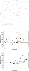 |
Fig. 3. Top panel: 2D map of the PSF FWHM variation across the g -band FOV of KIG 264. Middle panel: FWHM measured along the x-axis (RA) and along the y-axis (Decl., bottom panel) of this frame. The vertical red line marks the position of KIG 264. |
3.2. Data reduction
The photometric calibration, the point spread function (PSF) study and the surface photometric analysis were performed using Astronomical Image Decomposition and Analysis (AIDA) by Uslenghi & Falomo (2011). This software package, written in IDL (Image Display Language), was originally designed to analyse images of galaxies with a bright nucleus and to decompose them into the nuclear and galaxy components. AIDA includes tools for PSF characterisation.
Because of the photometric instability and owing to the full-sky coverage of the SDSS survey (York 2000), we corrected the calibration of our g- and r-band images by comparing the photometry of stars in each field with their SDSS magnitudes. Using the SDSS navigator tool, we inspected each target field and identified a set of stars nearby the galaxy. We bootstrapped our instrumental magnitude of these isolated unsaturated stars to their corresponding g and r SDSS magnitude in the star catalogue. The instrumental stellar magnitude in AIDA was calculated within different apertures in order to include the entire star, while the nearby residual sky was calculated in a ring cleaned from possible faint nearby stars and objects. The adopted zero-points (ZPs hereafter) and their errors, reported in Col. 6 of Table 3, are the average values and the standard deviation of the scatter in magnitude of the set of stars used.
The PSF shape was obtained from the same set of stars for each g and r field. AIDA characterises the PSF using 2D models (both analytical and empirical, or a combination of them), even when they are variable in the FOV. PSF models can be provided by the user or modelled by AIDA itself using reference stars in the images. Figure 4 shows one of the stars we used to obtain the PSF in the analysis of KIG 264. Although characterisations of PSF models exist (three Gaussians plus an exponential) up to large radii (several arcminutes; Slater et al. 2009; Sandin 2014; Trujillo & Fliri 2016; Karabal et al. 2017; Infante-Sainz et al. 2020, the relatively small extent of our targets means that the analytical PSF model that is adapted is indeed extended to the galaxy outskirts to obtain seeing-corrected parameters (Sandin 2015).
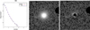 |
Fig. 4. PSF in KIG 264 in the g band. The 2D PSF is best fitted with a composite model (solid line) combining three Gaussians plus an exponential. The adopted PSF has been generated from a set of stars (star 6 is shown) close to the galaxy. The seeing correction is extrapolated up to the galaxy outskirts (see the discussion in Rampazzo et al. 2019, and references therein). A masked star is visible on the NW side of the field. |
For target galaxies, as in the case of stars, the residual sky background was determined within a ring of variable radius, well outside the galaxy and its peculiar outskirts, masking sources within it. Only a few very extended galaxies are crossed by the CCD gap. This latter was masked during the reduction and analysis procedure. The sky background value was obtained as the average of sectors of the ring, and the errors are the standard deviation of averages. AIDA also provides the radial light profile, with associated measurement errors, of the objects. The radial profile is computed by averaging the signal within concentric rings centred on the galaxy. The standard deviation in the rings is then used to evaluate the error bars, after adding in quadrature the uncertainty on the sky background.
In the 2D approach (see also GALFIT by Peng et al. 2010 or IMFIT by Erwing 2015), all pixels, except for the masked pixels, contribute to the fitting process of the galaxy luminosity distribution, but suffer from the fact that the components have single fixed values for the ellipticity, position angle, and Fourier moments. The information about the variation with radius of the ellipticity, position angle, and isophotal shape parameters obtained from the analysis of the galaxy azimuthal luminosity profile (see e.g. Jedrzejewski 1987) is lost. In modelling the galaxy light profile, AIDA adopts two values of the ellipticity and position angle in the case of a bulge plus disc (B+D) decomposition. Before the analysis of our target galaxies, the masking of the foreground and background objects superposed on the target galaxy was also performed manually, that is, masks were tailored to the extension of the objects that were to be removed. The fitting algorithms used by AIDA are MPFIT (Markwardt 2008) and a modified version of the IDL standard library function CURVEFIT, which uses a gradient-expansion algorithm (based on CURFIT; Bevington 1994). The original algorithm was modified in order to allow boundary constraints on the parameters.
3.3. Data analysis
Our scientific aim is twofold: to unveil fine structures, and to quantitatively refine the galaxy morphology given in Table 1. The sample is composed of Es and S0s to about the same portions. However, the three classifications considered in Table 1 often differ significantly, as shown in Fig. 1. To ascertain the presence of a disc is very valuable information about the role of dissipative processes in the ETGs evolution. We are aware that the photometric evidence is, however, a necessary but not sufficient condition (see e.g. Meert et al. 2015; Costantin et al. 2018, for an ample discussion) to determine the presence of a kinematical disc.
We remark that our purpose does not consist of introducing additional functions to possibly best fit regular features (e.g. analytic functions to mimic a bar, rings etc., as e.g. in GALFIT or IMFIT approaches). On the one hand, the fine structure we aim to reveal, such as shells, ripples, and tails, are often if not always irregular. Fine structures should be visible in the image itself. Fitted models are intended to enhance fine structures when they are subtracted from the original image. On the other hand, the visual classification in Table 1 reports only few iETGs with a ring or bar, or mixed AB types in the Buta et al. (2019) classification. In addition, the galaxies that are acknowledged to possess these features are not necessarily the same in the three classifications presented in Table 1. Only KIG 264 is considered barred by Buta et al. (2019), while KIG 264, KIG 620, and KIG 636 for HyperLeda are barred S0s. Buta et al. (2019) considered KIG 620, KIG 636 and KIG 733 as mixed AB type. Some of these galaxies have an inner ring. Only KIG 733 for Buta et al. (2019) and KIG 599 and KIG 644 for HyperLeda possess outer rings.
To conclude, we are aware that bars and inner rings introduce an erroneous evaluation of the bulge parameters if they are not considered in the fit. Meert et al. (2015) remarked that the presence of a bar affects the fitting by changing the ellipticity and Sérsic index of the bulge component in their two-component models. However, the classifications severely differ in our case, so that the presence of bar and rings needs to be carefully determined by our surface photometry. Our results are described in detail in Sect. 4.2.
We used two models to best fit the galaxy light profile. We best fit a single Sérsic law (Sérsic 1968), which is intended to represent Es (see e.g. Ho et al. 2011; Li et al. 2011, and reference therein) and a classic bulge (de Vaucouleurs 1953) plus an exponential disc (Freeman 1970), labelled B+D hereafter, for disc galaxies. The Sérsic law exponent was left free to vary up to n ≤ 10 in the single Sérsic fit (the values n = 1 and n = 4, the Freeman and de Vaucouleurs laws, respectively, are special cases). The selection of the B+D model is justified by the following consideration that takes into account that our range of morphological type is −5 ≤ T ≤ 0 according to Fernandez-Lorenzo et al. (2012), which we used for sample selection. Large surveys based on SDSS, which used automated decomposition algorithms, widely debated the biases introduced in the galaxy final structural parameters by fitting the light profiles using different models, mostly in connection with image resolution and galaxies with B/T ≤ 0.5 (see e.g. Gaditti 2009; Simard et al. 2011; Meert et al. 2015). Our targets are nearby (see Table 1), extended, and relatively bright galaxies (see Table 2). The galaxy light is dominated by the bulge (the average is ⟨B/T⟩ = 0.67), as discussed in Sect. 4. Meert et al. (2015) showed that B/T, bulge radius, and bulge Sérsic index all decrease with increasing T-type. The median bulge Sérsic index in their fit of a Sérsic plus exponential disc for the earliest T-types (−5 ≤ T ≤ 0) is approximately 5.0 ± 1.5 (see their Fig. 23), which is fully consistent with our use of a de Vaucouleurs law. Their median B/T decreases from 0.8 to 0.5 over the same range as in our case (see our Sect. 4).
The fit quality, as described in Uslenghi & Falomo (2011), was estimated by minimising the χ2. In AIDA, the minimised χ2 is defined as
 (1)
(1)
The masked pixels are excluded from the fit. The weighted model is computed defining σx, y as the sum in quadrature of three distinct components with different dependence on the signal level,
 (2)
(2)
C, SY, and α can be provided either by the user or they can be computed by AIDA based on readout noise and gain. If SY = α = 0, the fit is unweighted. In general, C describes the constant component of the noise, which is independent of the signal (in the ideal case, it coincides with the readout noise, without sky background), SY describes the component proportional to the square root of the signal (shot noise, in this case, SY is related to the conversion factor Ke-/ADU), and α represents the fixed pattern noise. We selected the weighted fit in both Sérsic and B+D models, tailored to the 4KCCD.
Meert et al. (2015) noted that when multiple components are fitted, a significant second component may only indicate substantial departure from a single-component profile rather than the presence of a physically meaningful second component. They quoted as examples Gonzalez et al. (2005), Donzelli et al. (2011), and Huang et al. (2013), who fitted multiple components to ellipticals (E) and bright cluster galaxies without necessarily claiming the existence of additional physically distinct components. Our data set is deeper than the SDSS data set, and this significantly affects the model selection. The single Sérsic fit often tends to overestimate the galaxy luminosity at low surface brightness levels, for instance, also when fine structures are present. The effect on the magnitude estimate is weak, but the B+D model is statistically better by far (even by eye) in describing the galaxy light profile for most of our iETGs. The images in g and r bands of the iETGs in our sample and a summary of the analysis performed are collected in Fig. 5 and in Appendix A.
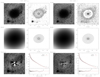 |
Fig. 5. Summary of the g− (left panels) and r− (right panels) band surface photometry of KIG 264. The adopted masks of the foreground and background objects are not shown. North is up, and east is to the left. The right panels provide from top to bottom (left) the original image, the best-fit model image, and the image of residuals after model subtraction for the g band. (right) Isophotal contours of the image, of the model, and of the azimuthal light profile. For clarity, only the model (red line) is over-plotted on the azimuthal light profile, and the (O–C) residuals are shown. Table 4 reports the model parameters. We show 20 isophote levels, between 500 and 2 σ of the sky level (μg = 21.6 ± 0.02 and 26.9 ± 0.34 mag arcsec−2 and μr = 21.0 ± 0.02 and 26.6 ± 0.29 mag arcsec−2), for the original and model images. The same panels are shown for the r-band photometry. KIG 264 reveals ripples and tail at the NW side of the galaxy body and a shell system in the outskirts. These features are revealed in both the g and r images above 2σ of the sky level and in the light profiles, starting at ≈30″. |
4. Results
Table 4 reports the seeing-corrected parameters derived from the Sérsic and/or the B+D light profile best fit. The table columns are described in the table caption. Columns 12 and 13 report the morphological class we assigned and the notes about the morphology of the residuals after model subtraction. We adopted the following criteria to assign the morphological class: We classified as S0 (-2 < Type ≤ 0) galaxies whose profiles were best fitted by a B+D model and have 0.5 < B/T ≤ 0.7, and we classified as E/S0 (Type = −3) galaxies with 0.7 < B/T < 0.8 (see e.g. Meert et al. 2015, their Fig. 23). Galaxies whose luminosity profile was best fitted by a single Sérsic law (i.e. by definition, B/T = 1) were classified as E (−5 < Type < −4). We considered that a nearly pure disc galaxy has a Sérsic index n ≈ 1 (i.e. by definition, B/T ≈ 0). We added the notation “pec” to the classification when galaxies have structured residuals.
KIG photometric data from the adopted Sérsic and B+D best-fit models and morphological notes.
Uncertainties for the bulge and disc effective radii, ellipticity, and position angles for the adopted models were obtained using the Monte Carlo simulation method. Noise and the uncertainty in the sky level determination were added. The errors on ellipticity, position angle, bulge effective radius, etc. quoted in the table are based on variables that do not depend on the model, in this case, Poisson noise. More realistic errors are likely larger. This can be verified by comparing the values among the bands: the differences may reach 10%, which is common for this type of model fitting.
4.1. Comparison with the literature
In Fig. 6 we compare the difference between our total integrated magnitudes, reported in Table 4, and the g and r bands from SDSS DR16 (Table 2). Our magnitudes are brighter on average by 0.10 and 0.09 mag in g and r bands, respectively. This value is higher than the measurement errors. KIG 637, which is not included in Fig. 6, presents integrated magnitude values that differ largely (≈0.46 mag) from the SDSS DR16 values. The excess in magnitude in our measures in this case is partly associated with the diffuse light of HD 238370, a very bright nearby star that cannot be properly modelled and subtracted. The extension of the stellar corona is visible in the top panels of Fig. A.6, showing g and r residuals.
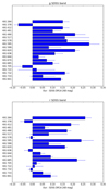 |
Fig. 6. Comparison between our integrated magnitudes in g and r bands with the SDSS DR16 values reported in Table 2. The solid lines show our errors. KIG 637 is not plotted because the magnitudes are strongly influenced by the nearby bright star HD238370 (see Sect. 4.2). |
Comparisons with other photometric works and/or recent photometries are difficult for the following reasons: (1) our values refer to either a simple Sérsic law or to a B+D decomposition, that is, they are tied to the adopted model, and (2) our photometry is deeper, for example, than data sets extracted from SDSS images, for instance. The ellipticity, ϵ, and the position angle, PA, of our models are not directly comparable with the values provided in Table 2. We averaged the g− and r-band values of ϵ and of PA for each galaxy. These results are in general comparable with the ϵ and PA data in Table 2. Our PA of the bulge, 102.7 ± 1.1 and 103.1 ± 1.1 in g and r band, and of the disc, 99.8 ± 1.1 and 100.4 ± 1.1, of KIG 637 (NGC 5687) compares well with 103.6 ± 0.01 and 101.2 ± 0.1 provided by the two Sérsic-law fits by Costantin et al. (2018). The same holds for the ellipticity of the bulge, 0.40 ± 0.04 in both bands, and of the disc 0.36 ± 0.03 and 0.37 ± 0.03 in g and r bands compared with 0.314 ± 0.001 and 0.338 ± 0.001 by Costantin et al. (2018).
The parameters of the 2D galaxy model, provided in Table 4, are complemented by Figs. A.1–A.9 in Appendix A. The caption of Fig. 5 details the information provided by the galaxy modelling. Our interest in particular is the detection of the galaxy fine structure, such as stellar tails, streams, fans, and shells. The light-profile fit and the residuals after the 2D model subtraction are shown for each band in the bottom panels of these figures.
The (g − r) colour profiles are collected in Fig. 7. In Fig. 8 the colour profiles are divided into three categories and plotted using a kiloparsec scale in the abscissa. In discussing (g − r) colour profile, we recall that because the flat field is imperfect, we had to fit the background with SWarp (Bertin et al. 2002) (see Sect. 3). This might influence the colour profile in the low surface brightness regimes, where the errors are indeed quite large. Outside the seeing region, the trend of the vast majority (see the middle panel) of the colour profiles is flat, with values typical of ETGs, that is, around 0.7–0.8 mag. The colour profiles of KIG 264 and KIG 378 (g − r) are shown in the top panel. They tend to become redder with radius. The bottom panel includes colour profiles either with peculiar trends, such as those of KIG 636 and KIG 841, or profiles that become bluer with radius. Single colour profiles are discussed in Sect. 4.2.
4.2. Individual notes
In this subsection we discuss the results summarised by the figures in Appendix A. Detailed surface photometric studies have been dedicated to some of the iETGs we study here by H-T, Rampazzo et al. (2019) in the K band and by Costantin et al. (2018) in the SDSS i band. Automatic surface photometry and 2D luminosity profile decomposition in these SLOAN bands have also been performed for some objects by Simard et al. (2011) and by Meert et al. (2015). In our discussion of the (g − r) profile, we exclude values with a radius below three times the FWHM, which are perturbed by the seeing, and measurement in the outskirts with errors larger than 0.3 mag.
KIG 264. The galaxy is considered a barred lenticular by Buta et al. (2019) and HyperLeda classifications, as a mixed E/S0 by Fernandez-Lorenzo et al. (2012), and as an E by H-T. The fit with a single Sérsic law provides a poor fit of the light profile; a B+D model (see Fig. 5) gives a statistically much better representation. Our surface photometry suggests the presence of a disc, but we did not find evidence of a bar. The cross-like shape in the g and r residuals in the inner regions (see Fig. 5) is an artefact due to the boxy shape of real isophotes with respect to our model. The isophotes boxiness has previously been noted by H-T. In the NW, the SE and NE residuals (Fig. 5) compose a shell structure. A fan, likely a wide tail, starting from the galaxy body, is attached to the NW part of the shell structure. These features have not been detected in the study by H-T. The B+D model fits the luminosity profile well up to the fan that appears as an increase of the disc surface brightness starting at ≈30″ in the g and r bands. The B/T = 0.68 in both bands indicates that the bulge component is dominant. We suggest that the galaxy is a peculiar unbarred S0. The (g − r) colour profile grows monotonically from ≈0.5 mag to unusually high red values in the galaxy outskirts, which may suggest the presence of dust.
KIG 378. The galaxy is classified as an elliptical by Buta et al. (2019) and HyperLeda, but it is considered as an E/S0 by Fernandez-Lorenzo et al. (2012) and as a S0 by H-T. The luminosity profile is statistically best fitted by a B+D model (Fig. A.1). The exponent of the single Sérsic-law fit is n ≈ 3, although the model tends to overestimate the galaxy luminosity in the outskirts. The bulge dominates in the adopted B+D best fit. It remains unclear why the B/T light ratio, which is 0.63 in g and 0.78 in r, differ so much although the fit is good in both cases. A residual structure (a tail?) extending from the nucleus towards the NW, which is particularly evident in the r band, is revealed after the model subtraction. We classify this galaxy as S0 pec, taking into account the asymmetric residual structure. The (g − r) profile is nearly flat at about 0.8 mag up to 17″, and then it becomes redder and reaches ≈1 mag at about 20″, where there are significant measurement errors, however.
KIG 412. The galaxy is one of the less isolated galaxies in the sample (Fig. 2) for Verley et al. (2007a), but the spectroscopic criterion of Argudo-Fernàndez et al. (2013) is fulfilled. All classifications in Table 1 converge in indicating this galaxy is an E, but it is an S0 galaxy for H-T. The single Sérsic fit provides n = 4.38 ± 0.11 and n = 5.80 ± 0.02 in g and r bands, respectively. However, this model not only overestimates the luminosity in the galaxy light profile in the outskirts, but the trend of the residuals also suggests the presence of a second component. The B+D provides a statistically better fit (Fig. A.1 bottom panel), as in the case of KIG 378. The residuals after the B+D model subtraction show a faint inner ring and a ring or shell-like structure in the outskirts (similar to KIG 685). Although this latter structure is revealed below 2σ of the sky level, it is evident in both original images, especially in the r band, starting from ≈20″. Our surface photometry supports an E/S0 pec classification because the bulge is still dominant; B/T is 0.69 and 0.71 in the g and r bands, respectively, and residual structures are present. The (g − r) colour profile is nearly flat at about 0.8 mag.
KIG 481. The galaxy has a very uncertain classification. It is an SA (T = 1) for Buta et al. (2019), an Sab for H-T, a late S0 (T = −0.1) for HyperLeda, and a classic S0 (T = −2) for Fernandez-Lorenzo et al. (2012). Morales et al. (2018) found two classical shells on either side of the galaxy. Our best fit (Fig. A.2) is obtained using a B+D model with a B/T = 0.66 and B/T = 0.69 in g and r bands, respectively. Residuals show a strong irregular dust-lane and a wide system of three nearly concentric shells. We suggest that it is a S0 pec (see also Buta et al. 2019). The galaxy (g − r) colour profile is quite blue in the galaxy centre, it is 0.64–0.7 mag, and it tends to become bluer with radius.
KIG 490. The galaxy is considered a late-S0 (Table 1) and an Sa for H-T. In Fig. A.2 we show our B+D best fit of the galaxy light profile. Residuals show a wide plume, likely a tail, in the NE part of the galaxy starting at about 30″ from the nucleus. The feature is reminiscent of the fan or tail found on the NW side of KIG 264 and connected with the shell. The B/T ratio (0.50 in g and 0.53 in r) together with the ripple and tail we detected fully justify the Buta et al. (2019) classification of a late, un-barred, and peculiar S0. The (g − r)≈0.74 mag colour profile is typical of ETGs (Fig. 8 bottom panel).
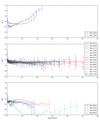 |
Fig. 8. (g − r) colour profiles in kpc (using the galaxy distance provided in Table 1). Colour profiles have been subdivided into three classes according to their behaviour outside the seeing-dominated area: galaxies with colour profiles become redder with radius (top panel), flat colour profiles (middle panel), and colour profiles with a peculiar behaviour or that become bluer in the outskirts (bottom panel). |
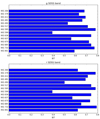 |
Fig. 9. Distribution of B/T in the g (top panel) and r bands. The average B/T values is 0.66 in both bands. |
KIG 517. This galaxy is considered a classical E by Buta et al. (2019) and H-T and an S0 by HyperLeda and Fernandez-Lorenzo et al. (2012). H-T found that it has a boxy structure that we do not see in either the original isophotes or as an artefact in the residuals. The single Sérsic best fit provides n values near to a de Vaucouleurs law. Our B+D model (Table 4) subtraction (Fig. A.3) shows a faint residual ring in the range 5–10″. The B/T values are 0.71 and 0.74 in g and r, respectively, indicating a large bulge contribution. We suggest that the galaxy is an E/S0. The (g − r) colour profile is flat around 0.75 mag.
KIG 578. The galaxy is classified E by all authors in Table 1 and by H-T, who detect a discy structure in isophotal shape profiles. The best fit is obtained with a single Sérsic law, with n ≈ 4; the B+D model best fit is statistically poorer. The residuals after model subtraction shown in Fig. A.3 reveal a ring between ≈10″-20″ and a faint outer ring or shell-like structure, detected at 2σ of the sky level, in the galaxy outskirts. KIG 578 is in the bona fide Es sample of H-T, and they did not detect shells in their SDSS image. We suggest that KIG 578 is a peculiar elliptical. The (g − r) colour profile is flat around 0.86 mag.
KIG 595. The galaxy is classified an E by Buta et al. (2019) and HyperLeda and as an S0 by Fernandez-Lorenzo et al. (2012) and as an SAB0 by H-T. The light profile is best fitted by a B+D model with a B/T = 0.78 in both bands. The residuals in Fig. A.4 show a faint inner ring and a series of shells that connects in the north to a tail (below 2σ level) that extends to the NW. No bar is revealed. We suggest that the galaxy is an E/S0 peculiar. The (g − r) colour profile is flat around 0.80 mag.
KIG 599. Classifications in Table 2 see the galaxy as a S0, but it is an E with discy isophotes and a system of shells and ring for H-T. A B+D model fits the galaxy best. Residuals after model subtraction show an arm-like structure in the inner part, and shells and a faint ripple on the SE side of the galaxy, emerging at about 40″ in both bands (Fig. A.4). We suggest that the galaxy is a peculiar S0, likely late, because B/T = 0.39 as in Fernandez-Lorenzo et al. (2012). The (g − r) colour profile is flat around 0.77 mag.
KIG 620. The morphological type of this galaxy ranges from −2 to 1 ± 1.6, suggesting that its is a late-S0 or an early spiral. According to HyperLeda, the galaxy hosts a bar. H-T classifies the galaxy as an early spiral (T = 0.69). Our image shows that KIG 620 is composed of a inner disc, seen nearly edge-on, with ϵ = 0.72, which is embedded in a diffuse nearly round structure (top panels in Fig. A.5). The Sérsic and B+D models both provide a poor fit: the bulge is small, and the parameters are largely contaminated by the inner ring. We support the Buta et al. (2019) classification because we do not see a bar. No fine structures are detected at a significant level. KIG 620 is reminiscent of 3D early-type galaxies reported in Buta et al. (2015), whose prototypes are shown in their Fig. 23. The (g − r) colour profile is flat around 0.72 mag and tends to become bluer aound 0.5 in the outskirts, although the errors are large.
KIG 636. The galaxy is considered an S0 by the tree classifications in Table 2. It has a bar both for Buta et al. (2019) and for the HyperLeda classification. H-T classified the galaxy as E. Residuals from a Sérsic or a B+D model show the effect of a small bar or lens (clearly visible in the original central isophotes in both bands), and an outer ring from which extended arm-like structures (tails?) depart, with arms on the E and W sides of the galaxy. The bulge parameters are contaminated by the bar in this case as well. We modelled the galaxy to enhance the outer galaxy structures. The classification of Buta et al. (2019) describes the inner morphology of the galaxy (T = −2.5) well, B/T = 0.74 would suggest T = −3 of Fernandez-Lorenzo et al. (2012). The suffix “pec” is necessary because of the arm-like residual structures. The increasing reddening, from ≈0.4 to 1 mag, of the (g − r) colour profile is connected to structures detected in the residuals map up to about 10″. After this, the (g − r) trend inverts and becomes increasingly blue. It reaches 0.6–0.5 mag, although with large errors, in correspondence to the outer ring and arm-like structures.
KIG 637. The galaxy is classified as an elliptical in Table 1. Recently, Costantin et al. (2018) reported the i- SDSS band surface photometry of this galaxy (NGC 5687 in the paper) and found that it is an S0 whose bulge can be unambiguously classified as classical (n > 2), with an n = 2.58 ± 0.0. This galaxy was chosen by Costantin et al. (2018) because it is unbarred.
Several bright stars in the field, in particular, HD238370, which generates a very extended corona, hampered the surface photometry and the estimate of the value of the total integrated magnitudes provided in Table 4. The galaxy extends ≈2.5′ in radius. We fit the entire light profile with a Sérsic law (n = 3.92 and n = 4.09 in the g and r bands, respectively). The index would suggest a classical E galaxy. However, the B+D model provides a better fit of the light profile. Residuals reveal a ring structure in the galaxy centre. This does not seem an artefact because this feature is also visible in i bands by Costantin et al. (2018) after the subtraction of their Sérsic+exponential disc model. Our measured PA = 102° and ellipticity ϵ = 0.39 (see Table 4) agrees with those found by the above authors. We suggest that the galaxy is an S0 (B/T = 0.57) whose inner and outer rings are revealed by the residuals. The (g − r) colour profile is nearly flat at ≈0.78–0.74 mag, without a signature of the structure detected in the residuals, and it tends to become bluer in the outskirts and reaches 0.6 mag with large errors.
KIG 644. The galaxy morphological type has a wide range of variation −1 ≤ T ≤ 2.2. The galaxy is considered borderline with a spiral: H-T classified it as Sab(s). As in the case of KIG 620, we failed to fit the light profile: both Sérsic and B+D model offer quite a poor fit. In the inner regions lies a ring-like structure with a diameter of about 10″ that hampered the fit of a very small bulge. Our images reveal neither spiral arms, as assumed by HyperLeda and H-T, nor fine structures such as shells and tails in the outskirts. We consider the classification provided by Buta et al. (2019) adequeate. The authors suggested a ring-like feature that outlines a bar that might be related to the x1 family of bar orbits as in NGC 6012 (see e.g. Buta et al. 2015, for an explanation). We assigned S0 as the morphological class. The (g − r) colour profile is nearly flat around 0.77 mag with large errors, without a signature of a ring.
KIG 670. The galaxy classification ranges from pure E to classic S0. A B+D model fits the light profile best. After model subtraction, the residuals show central asymmetries that are due to isophote twisting that is not accounted for in the model. In the outskirts, however, asymmetries (shells or ripples?) are visible in both bands (Fig. A.6). We suggest that the galaxy is an E/S0 pec as a consequence of a B/T = 0.73 and of the peculiar outskirts. The (g − r) colour profile is nearly flat around 0.82 mag.
KIG 685. The galaxy is considered a bona fide elliptical. H-T considered the galaxy an S0, however. Rampazzo et al. (2019) fit the high-resolution (PSF = 0 25) K-band 2D light distribution best with GALFIT, adopting a model composed of two Sérsic laws representing a pseudo-bulge (n = 2.95 ± 0.10) plus a disc (n = 0.78 ± 0.10). The ellipticity profile, showing two regimes, suggested the presence of the disc. KIG 685 K-band residuals show ring and shell-like structures. Our surface photometry is heavily hampered by bright stars that are located very near the galaxy centre. The PSF (see Table 3) is between 3.5 (g band) and 4.8 (r band) times that of ARGOS+LUCI adaptive optics instrument at the LBT. Our g and r study confirms the disc, the shell and ring-like structures that were detected in the previous study, as shown in Fig. A.6. We suggest that the galaxy is a peculiar E/S0. The (g − r) colour profiles is nearly flat at ≈0.88 mag.
KIG 705. This galaxy is also considered an E (see Table 2), including H-T, who in addition reported a discy structure of the isophotes, an inner disc, and shells and ripples. A Sérsic model fits the galaxy best, with n = 3.61 ± 0.03 in g and n = 4.07 ± 0.08 in r, supporting the idea that this is a classic E (top panels of Figures A.8). The B+D model, which is statistically indistinguishable from the previous model, offers a B/T = 0.89 in both bands, suggesting in any case that the bulge component is dominant. The residuals after model subtraction enhance shells and ripples in the galaxy outskirts. The galaxy shows a disc-like structure in the inner region. We assigned E pec as the morphological class. The (g − r) colour profiles are nearly flat around 0.77 mag.
KIG 722. The galaxy is considered a bona fide E with boxy isophotes according to H-T. Our best-fit model is a Sérsic law in both bands with exponents near the classic de Vaucouleurs law (see Table 4). The residuals (bottom panels of Fig. A.8) in the central part of the galaxy therefore are an artefact created by the combination of the isophote twisting and boxiness with respect to the model. The excesses of light between 20″-40″ at the NE and SW sides of the galaxy appear as real fans and shells that are also visible in the original image. H-T did not detect shells in their SDSS image of KIG 722. We assigned E pec as the morphological class. The (g − r) colour profiles are nearly flat around 0.76 mag without any obvious connection with the structure that is enhanced by the residuals.
KIG 732. This galaxy is another bona fide E in Table 2. H-T reported that this E has a boxy structure, dust, and possibly an inner disc. Our best-fit model is the B+D shown in Fig. A.9, although the bulge predominates (B/T = 0.88 and 0.78 in g and r bands). Isophotes appear strongly boxy: this is the reason for the cross-like residuals in the central regions of the galaxy. The residuals also enhance shells and a spiral-like structure that is likely due to isophote twist and extends out to the galaxy outskirts. We assigned the E/S0 pec morphological class. There are no traces in the nearly flat (around 0.77 mag) (g − r) colour profile of the structures that are traced by the residuals. H-T did not detect shells in their SDSS image of KIG 732.
KIG 733. The galaxy is borderline, with an early spiral (0 ≤ T ≤ 1.5) in the classifications provided in Table 1. Our B+D model fails to provide an adequate fit to the light profiles (bottom right panel in Fig. A.9). The galaxy has a complex morphology that is well described by the classification of Buta et al. (2019), with an outer ring starting from wide open arms. There is dust along the arms that appears knotty (see the bottom left panel). Considered as a whole, the galaxy is reminiscent of the 3D early-type objects in Buta et al. (2015), similarly to KIG 620. We suggest that the correct classification is provided Buta et al. (2019), so we assigned S0 pec as the morphological class. The (g − r) is red, nearly flat around 0.8 mag, with a mini peak of 0.94 mag at about 26″ in correspondence of the outer ring.
KIG 841. The galaxy is considered late-S0 (T = 0) in Fernandez-Lorenzo et al. (2012). For Buta et al. (2019), is also an S0, but with several peculiar features, such as an inner ring and plume, while it is an E/S0 for HyperLeda. Our surface photometry confirms the peculiar features in the Buta et al. (2019) classification. Furthermore, we find evidence of a wide systems of shells that is particularly evident on the NE side. Our best fit is obtained with a B+D model. The outer shells appear as an increase in luminosity in the model at ≈70″ at about 27 mag arcsec−2 in g band and 26 mag arcsec−2 in r band. We classify this galaxy as a late-S0 pec because B/T ≈ 0.6. The (g − r) colour profile (Fig. 8) is entirely unexpected for ETGs. Outside the seeing, it has values of about 0.6 mag, then it becomes increasingly bluer up to 25″, with a flat part at about −0.4 mag up to 50″. In the galaxy outskirts, the (g − r) trend turns to red, but the values are still below 0 mag.
To summarise, our light profiles reached on average μg = 28.11 ± 0.7 mag arcsec−2 and μr = 27.36 ± 0.68 mag arcsec−2. The results of the light-profile analysis decomposition are listed in Table 4. A minority, 15% (3 out of 20), of our iETGs can be considered bona fide Es that are fitted best by a Sérsic law with the exponent n≈4, that is, by a de Vaucouleurs law. For the vast majority, the B+D model fits the galaxy light profile best. The bulge flux is dominant, with an average B/T ≈ 0.66 in both bands. Three out of 20 iETGs, that is, NGC 620, NGC 644, and NGC 733, are late S0s at the border with spirals, some showing arm-like structures in their central region, as in the Buta et al. (2019) classification. On the whole, their morphology is reminiscent of the 3D ETG class described in Buta et al. (2015). We conclude that our sample is composed of bona fide ETGs.
After the 2D model was subtracted, most of the galaxies showed fine structures that emerged in their inner regions and outskirts. In particular, 12 out of 20 iETGs (60%) showed clear evidence of shell and ripple signatures (Table 4, Fig. 5, and Figs. A.1–A.9). None of the late S0s mentioned above show shells, ripples, or tails. In Sect. 2.2 we discussed the revised isolation criteria for the galaxy in the sample performed by Verley et al. (2007a) and Argudo-Fernàndez et al. (2013). Figure 2 shows that all iETGs with shells except for KIG 412 and KIG 595 lie within the fiducial range of isolation in the ηk-Q plane. This means that the fraction of shell galaxies within the isolation fiducial range reaches 62% (10 out of 16).
Most of the colour profiles, 13 out of 20 (65%), are flat with values in (g − r) of about 0.7–0.8 mag, which is typical of ETGs. Ten of the 12 shell galaxies have red (g − r) colour profiles; 2 galaxies, KIG 481 and KIG 841, have blue (and peculiar, in particular, KIG 841) colour profiles.
5. Discussion
By definition, iETGs are early-type galaxies without obvious companions. Considering the above results, the question is how long isolated early-type galaxies have been isolated. The answer, which involves both the timing and the physical mechanisms driving the iETG evolution, can be approached using the various fine structures that are detected as markers, together with other indicators that we discuss in the following sections.
5.1. Shapes of the residuals
Simulations suggest that the fine structures revealed by our surface photometry are connected to past interacting and merging history. We review the residual shapes and discuss them in the light of the literature.
5.1.1. Shells
In the literature, shells have been widely associated with both minor and major and both wet and dry merging episodes (see e.g. Dupraz & Combes 1987; Weil & Hernquist 1993; Mancillas et al. 2019; Pop et al. 2018, and references therein). Several studies have suggested that the fraction of shells, and in general, the fraction of tidal features, indicate a strong environmental effect. Reduzzi et al. (1996) found that about 16.5% of ETGs in the field showed shells, which is at odds with the hypothesis that 4% of ETGs are members of physical pairs. Only 4% of the shell galaxies in the original Malin & Carter (1983) list are located in clusters or rich groups. An incidence of 50% of shells has been found by H-T in 18 isolated galaxies that they considered bona fide Es, using the SDSS DR6 data set.
Our set of galaxies, however, needs to be compared with results from deep surface photometry because the fraction of detected features certainly depends on this factor. Tal et al. (2009) investigated a complete volume -limited (15–50 Mpc) sample of bright (MB < −20) ETGs and detected 12 out of 55 (22%) objects with shells. Their surface brightness reached 27.7 mag arcsec−2 in the V band. The authors noted that the fraction of galaxies with tidal features increased and did not include cluster members. We found that about 60% of our iETGs shows shell structures. With respect to H-T, we revealed shells also in KIG 264, KIG 578, KIG 722, and KIG 732, which are all included in their sample of isolated Es. Recently, Pop et al. (2018) investigated shells in 220 of the most massive galaxies, regardless of their environment, in the Illustris simulation (Genel 2014; Vogelsberger 2014a,b). They reported shells in 39 galaxies, which is 18 ± 3%. This fraction is consistent with the fraction found by Tal et al. (2009). The fraction of our iETGs that shows shells is three times greater than that found by Tal et al. (2009).
Most (9 out of 13) iETGs with shells have flat and red (g − r) colour profiles. This is consistent with the general finding that shells are more common in red than blue (spiral) galaxies (see e.g. Atkinson et al. 2013). KIG 481 and KIG 841, which have blue colour profiles, are still in the green valley (see Sect. 5.3).
The Mancillas et al. (2019) simulations suggested that shells are a long-lasting feature (see also Longhetti et al. 1999; Rampazzo et al. 2007). The estimated survival time of shells is ≈3 Gyr. Lacking possible perturbers, shells in our iETGs were generated by the last merging event and set the isolation time, which is of that order. Shells basically disappear in cluster ETGs, which likely is a consequence of the galaxy transformation due to continuous harassment processes (Moore et al. 1998). In less isolated ETGs (see Sect. 2.2), the fraction of galaxies with shells is still higher than the fraction quoted by Tal et al. (2009). Further indications about the age of the interaction are developed in Sect. 5.3.
Two of the iETGs with shells deserve further attention. KIG 264 shows a system of shells and a ripple that is reminiscent of a tail (Fig. 5). The galaxy has been studied at radio wavelength by Wong et al. (2015). They described KIG 264 (identified as J0836+30 in their paper) as the more passive object in their sample. They did not detect nuclear radio emission in the galaxy at 1.4 Ghz, but observed two radio lobes at 88.4 kpc north-west and 102.5 kpc south-east of the galaxy centre. In the direction connecting the two radio lobes, they detected an extragalactic H I cloud midway between the galaxy centre and the lobe on the north-west side (see their Figs. 2 and 5). Wong et al. (2015) suggested that an active central engine has the required energy to expel gas from the galaxy because two radio lobes are located in the same direction as the H I cloud. KIG 264 likely hosted a radio AGN that may have blown out the observed gas cloud.
Our surface photometry shows that KIG 264 has no bar that would drive gas to the centre. The wide system of shells extends to almost include the H I cloud. Because shells and ripples are the scars of a recent merging (see e.g. Mancillas et al. 2019), we suggest that this event has likely involved gas-rich galaxies (wet merging) and might have activated the past AGN activity in KIG 264.
KIG 264 shows the remains of the AGN activity, and the processes may occur during a merging episode. Bennert et al. (2008) found several cases of (active) AGN host galaxies with an underlying shell system. On the other hand, Hernàndez-Ibarra et al. (2013) found low AGN-level activity in our iETGs sample: only three galaxies, KIG 378, KIG 595, and KIG 705, have a low ionization nuclear emission line region (LINER) in the nucleus.
The other interesting case is KIG 841 (NGC 6524). The type Ia pec supernova SN2010hh exploded in its shell (Marion 2010; Silverman et al. 2010) (SN1991bg-like). The progenitors of this type of supernova are old stars, that is, stars that were likely re-distributed from the parent galaxies during the merging episode.
5.1.2. Tails, plumes, and fans
Tails of stellar matter are generated by interaction and merging phenomena (see e.g. Mancillas et al. 2019, and references therein). Broad stellar fans are also generated by interaction (see e.g. Tal et al. 2009). The tail survival time is ≈2 Gyr, while streams remain visible in all phases of galaxy evolution. Streams, however, are detected in simulations at very low levels of surface brightness. The Mancillas et al. (2019) simulations revealed between two and three times more streams with a surface brightness cut of 33 mag arcsec−2 than with 29 mag arcsec−2.
Tal et al. (2009) found that tails are less frequent than shells in ETGs: they found tails in 13% (7 out of 55) of the ETGs. Tails exist for shorter times than shells (Mancillas et al. 2019). Tails tend to indicate a recent encounter and/or merging. Furthermore, tails are evidence for a dynamically cold component (e.g. a disc).
We consider as tails, fans and plumes the features found in KIG 264, KIG 378, KIG 490, KIG 595, and KIG 636, that is, 25% (5 out of 20) of our sample. KIG 378, KIG 490, and KIG 636 were considered isolated by both Verley et al. (2007a) and Argudo-Fernàndez et al. (2013). All these galaxies are best fitted by a B+D model, which supports the idea described above that a cold disc structure is present.
5.1.3. Spiral arm-like residuals
KIG 599 and KIG 732 show shells and very wide spiral arm-like residuals on a very large scale. Arm-like structures are generated by an encounter that ends in a merger. The arm-like structure during the first phase, when the two nuclei are still visible, of both an encounter and a merging episode was shown in Combes et al. (1995), for instance. Clearly, KIG 732 is in an advanced merging phase. Residuals like this have been shown as residuals in other deep photometry (see e.g. Cattapan et al. 2019, in the case of NGC 1533). They were discussed as a signature of the disc instability during a merging episode (see e.g. Rampazzo et al. 2018; Mazzei et al. 2019).
5.1.4. Rings
When possible artefacts are excluded (see Sect. 4.2), several types of inner features become visible that are revealed in the residuals after model subtraction. Rings are one of the most frequent of these features, while bars are barely detected in the present sample.
Rings (inner and outer) are considered in the Buta et al. (2019) classification of isolated galaxies. Table 1 reports inner rings for four galaxies, KIG 481, KIG 490, KIG 620, and KIG 841, and a outer ring for KIG 733. The ring in KIG 481 (NGC 3682) is included in the Còmeron et al. (2014) catalogue among resonance rings in the Spitzer Survey of the Stellar Structure in Galaxies (S4G), where the galaxy is classified as SA(r)0+). After our model subtraction, the galaxy shows a strong central dust lane that perturbs the fit. It also shows concentric shell structures.
We detect inner ring-like structure in the KIG 412, KIG 517, KIG 578, KIG 620, KIG 636, KIG 637, KIG 644, KIG 685, and KIG 733 galaxies, of which seven fulfill the strict isolation spectroscopic criterion by Argudo-Fernàndez et al. (2013). In the cases of KIG 620, KIG 733, and KIG 733, which do not show obvious signatures of either interaction or merging, the rings may have been caused by resonances (Buta et al. 2010; Laurikainen et al. 2011, 2010). However, most of the detected rings are associated with other residual structures, such as shells or fan, that the literature assumes are merging signatures. Eliche-Moral et al. (2018) and Mazzei et al. (2019, and references therein) showed that the existence of embedded inner components, such as inner discs, rings, pseudo-rings, inner spirals, and nuclear bars at the centres of many S0s, which commonly are attributed to internal secular evolution, disc fading, or environmental processes, are compatible with a major-merger origin, including the relaxed and ordered discs of present-day S0s. Most of our iETGs show all these features, in combination with specific signatures of accretions/merging, such as shells. This corroborates this view.
5.2. H I content
The H I content of iETGs is important for at least two reasons. On the one hand, this content is connected to the ETGs environment, and on the other, to their evolutionary scenario. More specifically, because we found so many fine structures, the H I content is essential to distinguish between the wet versus dry version of the merging episode that iETGs appear to come from.
It has been known since the early 1980s that cluster spirals are gas anæmic with respect to their counterparts in a less dense environment (see the pioneering work of Giovanelli et al. 1982). ETGs, which as a family contain less H I than spirals, have only recently been found to share this property with spirals. This has been possible through high-sensitivity surveys. A significant fraction of ETGs in a low-density environment are more H I rich than cluster ETGs (10% in Virgo vs. 40% in the field) (see e.g. Serra et al. 2012). ETGs in a low-density environment may contain as much H I as a spiral galaxy.
Serra et al. (2012) found that as far as H I properties are concerned, the main difference between ETGs with large amounts of H I and spirals is that the former miss the high column density H I that is typical of the bright stellar disc of the latter. The star formation rate per unit area is much higher in spirals than in ETGs. Instead, Serra et al. (2012) concluded that the column density of H I found in ETGs is similar to the densities observed in the outer regions of spirals, which from a morphological and kinematic point of view show warps and other peculiarities that are connected to gas accretion. Serra et al. (2012) asserted that this is what is detected in H I-rich ETGs, that is, H I-rich ETGs and spirals may look very similar in their outskirts
We investigated if those of our iETGs that show many morphological disturbances are gas rich. The sample of observed iETGs is very small. Jones et al. (2018) recently presented the largest catalogue of H I single-dish observations of isolated galaxies as part of the multi-wavelength study of the AMIGA sample of isolated galaxies. Only two galaxies in our sample were detected in H I (CIG 264 and 481): KIG 685, and KIG 841. They lack H I data. The others have just 5σ upper limits. Based on the distances given in Table 1, Table 5 reports the measured H I masses (Col. 5) and the expected H I mass (Col. 6) according to the relations provided in Jones et al. (2018). With the iETG upper limits, the log MH I−pred provides values in the range of KIG 264 and KIG 418, that is, similar to median values for spirals (log MH I/M⊙ = 9.47, 9.84, and 9.59 for T≤, 3 < T < 5, and T ≥ 5, respectively). We are aware that the relations in Jones et al. (2018) were derived from a sample that is dominated by spirals because they are the vast majority of the AMIGA galaxies.
iETG H I content.
In the HI survey of ATLAS3D ETGs, Serra et al. (2012) observed KIG 637 (NGC 5687). They reported an upper limit that after adjustment to our distance (Table 1) and homogeneisation to Jones et al. (2018) is log MH I⟨8.12 M⊙. Serra et al. (2012) only detected about 40% of field ETGs, therefore this tight limit by itself does not suggest that other iETG are necessarily poor in H I.
We conclude that (1) for most of these iETGs, an H I component cannot be excluded because the expected HI content is generally below the upper limits of the surveys, and (2) the two existing detections in shell galaxies are in the range of the H I-rich ETGs in the Serra et al. (2012) data set.
5.3. iETGs in the (NUV-r) versus Mr colour magnitude diagram
Colour magnitude diagrams (CMDs hereafter), in particular those built in UV versus optical bands, have been shown to be a powerful tool for understanding the evolutionary phases of galaxies. In the plane Mr versus (NUV-r), galaxies occupy well-defined positions (see e.g. Wyder et al. 2007). Evolved galaxies, ETGs, and star-forming late-type galaxies are located in two well-populated and separated areas of the CMD called the red sequence and the blue cloud, respectively. The intermediate area, less populated by galaxies, has been labelled green valley (Kaviraj et al. 2007; Schawinski et al. 2007). This area is believed to be populated by transforming galaxies. Mazzei et al. (2019) showed the evolutionary path followed by galaxies when either encounter or mergers drive their evolution. Starting their evolution in the blue cloud as disc galaxies, they reach a point of maximum brightness before they start to quench their star formation and cross the green valley. They finally reach the red sequence and in the meantime modify their morphology and kinematic properties to become mature ETGs. The crossing time of the green valley depends on their mass (brightness). It lasts > 4 Gyr for the faintest ETGs.
Figure 10 shows the Mr versus (NUV-r) CMD of our targets. The dotted vertical lines, as derived from Fig. 8 in Mazzei et al. (2019), show the crossing time of the green valley as a function of the intrinsic brightest magnitude reached by simulated ETGs during their evolution in the blue cloud (see the quoted paper for a quantitative definition of different regions of the UV CMD and the evolutionary paths of the galaxies). All our iETGs have left the blue cloud. Some of them, both with and without a shell (red squares and orange dots, respectively), are still found in the green valley, but they mainly populate the red sequence.
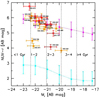 |
Fig. 10. UV-optical CMD of iETGs. In the Mr vs. (NUV-r) plane we plot the Wyder et al. (2007) fits to the red sequence (magenta dots and dotted line) and to the blue cloud (cyan dots and dotted line). iETGs with a shell system are indicated with orange dots. KIG 722 is missing from the iETGs sample because no NUV measures are available. The dotted vertical lines provide an indication of the green valley crossing time as a function of the galaxy luminosity (see text). The horizontal error bar accounts for a distance uncertainty of 10%. The vertical error bar accounts for the NUV ZP uncertainty, 0.15 mag (Bai et al. 2015). |
The Mazzei et al. (2019) smoothed particle hydrodynamics simulations with chemo-photometric implementation, anchored to global properties of 11+8 ETGs, showed that the luminosities of these ETGs fade away by 0.5 mag on average, after they reached the brightest point in the blue cloud, and the galaxies enter in the green valley. On this basis, the four iETGs in the green valley will spend between 1 up to 3 Gyr in this area before they reach the red sequence. iETGs that are located in the red sequence on average took less than 3 Gyr to reach it. However, it is unknown how long they have been and will remain in the red sequence. A careful analysis and a match of their global multi-wavelength properties are required to constrain our smoothed particle hydrodynamics simulations with chemo-photometric implementation, to understand their formation mechanisms and their evolutionary path (Mazzei et al. 2014b, 2019). This will be the subject of a forthcoming paper.
We investigated if iETGs in the red sequence are so-called red-and-dead systems. It is known that the star formation in ETGs in the red sequence cannot be entirely quenched because secondary episodes of star formation can still be revealed. Their signatures have been found from optical to UV and mid-IR wavelengths (see e.g. Annibali et al. 2007; Rampazzo et al. 2007, 2013; Panuzzo et al. 2007, 2011; Jeong et al. 2009; Salim & Rich 2010; Thilker et al. 2010; Marino et al. 2011a,b; Cattapan et al. 2019, and references therein). The Mazzei et al. (2019) simulations suggest that these phenomena are activated during the post-merging evolution of iETGs. In this context, KIG 264, a former AGN, has already reached the red sequence, where most of our iETGs are located, and it still shows the remains of this activity.
6. Summary and conclusions
We presented the morphological and photometric study of 20 iETGs from the AMIGA catalogue (Verdes-Montenegro et al. 2005) that are bona fide ETGs according to the revised classification of Fernandez-Lorenzo et al. (2012). The revised classification contains about 100 ETGs. Although the morphological classification has been revised both visually (Buta et al. 2019) and quantitatively (Hernández-Toledo et al. 2008) using SDSS, several discrepancies remain. One of our task has been to test the reliability of the above morphological classifications in the light of deep imaging in a quantitative way.
The AMIGA isolation criteria have been refined by Verley et al. (2007a) and by Argudo-Fernàndez et al. (2013). Four of the iETGs considered in this paper fulfil the Verley et al. (2007a) isolation criteria with a trend to present a larger number of minor companions (higher ηk value), while 10 out of 20 are strictly isolated for Argudo-Fernàndez et al. (2013) (who lack spectroscopic information for 4 galaxies in the sample, however), the other is expected to be only minimally affected by any neighbours. The iETGs in our sample are hence isolated from major companions and located in poorly populated environments.
Galaxies were observed in the g and r SLOAN bands at the 1.8m VATT telescope with the 4KCCD. The light profiles on the average reach μg = 28.11 ± 0.70 mag arcsec−2 and μr = 27.36 ± 0.68 mag arcsec−2, which makes this sample the deepest observations of iETGs so far. We used the AIDA package for the 2D photometric analysis and accounted for PSF effects during the decomposition of the light profiles up to the galaxy outskirts. We used the current literature to discuss thepg
morphology of the residuals obtained after the 2D model subtraction from the original image. We list our results below.
-
All the galaxies in the sample are bona fide ETGs, from Es to late S0s. None is a misclassified spiral.pg
-
Fourteen out of 20 iETG light profiles are best fit by B+D model.pg The average B/T is 0.66 in both bands, indicating that the bulge dominates the galaxy light distribution.pg H-T found that bona fide Es are rare among iETGs. KIG 578, KIG 705,pg and KIG 722 are best fit by a simple Sérsic law whose exponent is near to a classic de Vaucouleurs law (see Table 4). These galaxies are in the Es set of H-T. However, we fit KIG 264, KIG 599, and KIG 732 best with a B+D model. These galaxies are all in the H-T Es bona fide sample. Our B+D models failed to provide an acceptable description of the light distribution of iETGs with type close to 0, KIG 620, KIG 644, and KIG 733 because strong additional features such as one or more rings and wide arms are present in their central region. For the latter, Buta et al. (2019) provided the best classification. Their one or more rings may be interpreted in either the framework of resonances or other phenomena that have been described as a consequence of secular evolution (see e.g. Còmeron et al. 2014; Buta et al. 2010; Laurikainen et al. 2010, 2011) or as a consequence of merging (see e.g. Eliche-Moral et al. 2018; Mazzei et al. 2019, and references therein).
-
Most of our iETGs show fine structures such as shells, tails, residual faint rings, stellar fans, and a residual spiral arm-like structure after model subtraction. These features are considered signatures of accretion and merging events in the literature.
-
In 12 out of 20 (60%) of the iETGs, we detected shells. They compete with rings (10 out of 20) for the most frequently dectected fine structures (see also Tal et al. 2009). This percentage is confirmed also when we considered the set of iETGs that was smaller because stricter isolation criteria were used. H-T also found very many shell galaxies in isolated ETGs. However, in Table 6 of H-T, the detection of 4 out of 9 shells and ripples was uncertain, while we revealed shells in KIG 264, KIG 578, KIG 722, and KIG 732, which are listed in that table. This is expected because H-T used more shallow images (see the considerations in Mancillas et al. 2019).
-
Most (≈80%) of the iETGs are located in the red sequence in the (NUV-r) versus Mr CMD diagram. Seven out of 15 (KIG 722 lacks NUV data) show a shell structure. Four galaxies, that is, KIG481, KIG 620, KIG 705, and KIG 841, are still located in the green valley. Three of them have shells. Several other features connected to accretion and merging events are found in iETGs that are located in the red sequence.
-
Fourteen iETGs have nearly flat (g − r) colour profiles at ≈0.7–0.8 mag. These are normal values for early-type galaxies. We measured (g − r) colour profiles that become increasingly blue with radius for KIG 481, KIG 620, and KIG 841, at least in some regions. In contrast, quite red colours are measured in the outskirts for KIG 264 and KIG 378, suggesting the presence of dust. Dust is normally expected in the galaxy centre. In a small number of iETGs, the blue (g − r) colour profile may suggest a recent star formation episode by the high fraction of accretion and merging signatures. However, the time required to cross the (NUV-r) versus Mr plane from the green valley to the red sequence is relatively long, as shown in Fig. 10. This suggests that iETGs have had enough time to quench their star formation and AGN activity (as in KIG 264) in the case of wet mergers as well. This is in contrast to H-T and Tal et al. (2009), who suggested that dry mergers might provide a possible explanation of the evolution of these galaxies.
-
The prediction by Jones et al. (2018) about the H I content of our iETGs needs to be confirmed with deep 21 cm observations because they are based on a relation fit with a sample dominated by spiral galaxies. The wide morphological disturbance in the galaxy outskirts and the measure of MH I for KIG 264 and KIG 481 suggest that H I might have fuelled galaxy rejuvenation and AGN activity, as has been found in low-density environments (see e.g. Annibali et al. 2007, 2010).
The subsample of iETGs we studied presents a different behaviour from isolated late-type galaxies from the same AMIGA sample, showing a significantly higher number of perturbation signatures. Consistently, Fernandez-Lorenzo et al. (2013) found no difference in the stellar mass size relation between iETGs and counterparts in more dense environments, unlike late-type galaxies. We conclude that a significant fraction of our iETGs are a by-product of a merger. The high fraction of shells, a long-lasting fine structure in isolated and poorly populated environments, indicates that iETGs have not been perturbed for a long time (up to 3 Gyr). This is consistent with their degree of isolation. The crossing time required to move galaxies from the green valley to the red sequence in the Mr versus (NUV-r) CMD is consistent with this view. Shell galaxies that are found in the green valley will accumulate in the red sequence. Because of their isolation, iETGs appear as the cleanest environment for investigating a wide phenomenology (structure and sub-structure formation, duration, evolution, AGN feeding and fading, and star formation ignition and quenching) induced by both accretion and merging episodes.
Acknowledgments
A. O. and R. R. are deeply grateful to Fathers Richard Boyle SJ, Paul Gabor SJ and Jean-Baptiste Kikwaya SJ for assistance at the telescope. RR thanks the Specola Vaticana Director Brother Guy Consolmagno, Father Christopher Corbally and Father Thomas Williams SJ for the kind hospitality in Tucson (AZ-USA). R.R. and P.M. acknowledge funding from the INAF PRIN-SKA 2017 program 1.05.01.88.04. MGJ is supported by a Juan de la Cierva formación fellowship (FJCI-2016-29685). MGJ and LVM also acknowledge support from the grants AYA2015-65973-C3-1-R and RTI2018-096228-B-C31 (MINECO/FEDER, UE). This work has been supported by the Spanish Science Ministry “Centro de Excelencia Severo Ochoa” program under grant SEV-2017-0709. IRAF is distributed by the National Optical Astronomy Observatories, which are operated by the Association of Universities for Research in Astronomy, Inc., under cooperative agreement with the National Science Foundation. This research has made use of the NASA/IPAC Extragalactic Database (NED), which is operated by the Jet Propulsion Laboratory, California Institute of Technology, under contract with the National Aeronautics and Space Administration. We acknowledge the usage of the HyperLeda database (http://leda.univ-lyon1.fr).
References
- Abazajian, K. N., Adelman-McCarthy, J. K., Agüeros, M. A., et al. 2009, ApJS, 182, 543 [NASA ADS] [CrossRef] [Google Scholar]
- Akhlaghi, M., & Ichikawa, T. 2015, ApJS, 220, 1 [NASA ADS] [CrossRef] [Google Scholar]
- Atkinson, A. M., Abraham, R. G., & Ferguson, A. M. N. 2013, ApJ, 765, 28 [NASA ADS] [CrossRef] [Google Scholar]
- Argudo-Fernàndez, M., Verley, S., Bergond, G., et al. 2013, A&A, 560, A9 [NASA ADS] [CrossRef] [EDP Sciences] [Google Scholar]
- Argudo-Fernàndez, M., Verley, S., Bergond, G., et al. 2015, A&A, 578, A110 [NASA ADS] [CrossRef] [EDP Sciences] [Google Scholar]
- Arp, H. 1966, ApJS, 14, 1 [NASA ADS] [CrossRef] [Google Scholar]
- Annibali, F., Bressan, A., Rampazzo, R., Zeilinger, W. W., & Danese, L. 2007, A&A, 463, 455 [NASA ADS] [CrossRef] [EDP Sciences] [Google Scholar]
- Annibali, F., Bressan, A., Rampazzo, R., et al. 2010, A&A, 519, A40 [NASA ADS] [CrossRef] [EDP Sciences] [Google Scholar]
- Bai, Y., Zou, H., Liu, J., et al. 2015, ApJS, 220, 6 [NASA ADS] [CrossRef] [Google Scholar]
- Bennert, N., Canalizo, G., Jungwiert, B., et al. 2008, Mem. Soc. Astron. It., 79, 1247 [NASA ADS] [Google Scholar]
- Bertin, E., Mellier, Y., Radovich, M., et al. 2002, Astron. Data Anal. Softw. Syst. XI, 281, 228 [Google Scholar]
- Bevington, P. R. 1994, Data Reduction and Error Analysis for the Physical Sciences (McGraw-Hill) [Google Scholar]
- Buta, R. J., Seth, K., Athanassoula, E., et al. 2015, ApJS, 217, 32 [NASA ADS] [CrossRef] [Google Scholar]
- Buta, R. J., Verdes-Montenegro, L., Damas-Segovia, A., et al. 2019, MNRAS, 488, 2175 [Google Scholar]
- Buta, R. J., Laurikainen, E., Salo, H., & Knapen, J. H. 2010, ApJ, 721, 259 [NASA ADS] [CrossRef] [Google Scholar]
- Cappellari, M. 2016, ARA&A, 54, 597 [NASA ADS] [CrossRef] [Google Scholar]
- Cattapan, A., Spavone, M., Iodice, E., et al. 2019, ApJ, 874, 130 [NASA ADS] [CrossRef] [Google Scholar]
- Clemens, M. S., Bressan, A., Nikolic, B., et al. 2006, MNRAS, 370, 702 [NASA ADS] [CrossRef] [Google Scholar]
- Clemens, M. S., Bressan, A., Nikolic, B., & Rampazzo, R. 2009, MNRAS, 392, L35 [NASA ADS] [CrossRef] [Google Scholar]
- Combes, F., Rampazzo, R., Bonfanti, P. P., Pringniel, P., & Sulentic, J. W. 1995, A&A, 297, 37 [NASA ADS] [Google Scholar]
- Còmeron, S., Salo, H., Laurikainen, E., et al. 2014, A&A, 562, A121 [NASA ADS] [CrossRef] [EDP Sciences] [Google Scholar]
- Costantin, L., Corsini, E. M., Méndez-Abreu, J., et al. 2018, MNRAS, 481, 3623 [NASA ADS] [CrossRef] [Google Scholar]
- Côtè, P., Piatek, S., Ferrarese, L., et al. 2006, ApJS, 165, 57 [NASA ADS] [CrossRef] [MathSciNet] [Google Scholar]
- de Vaucouleurs, G. 1953, MNRAS, 113, 134 [NASA ADS] [CrossRef] [Google Scholar]
- Donzelli, C. J., Muriel, H., & Madrid, J. P. 2011, ApJS, 195, 15 [NASA ADS] [CrossRef] [Google Scholar]
- Dressler, A. 1980, ApJ, 236, 351–365 [NASA ADS] [CrossRef] [Google Scholar]
- Duc, P.-A., Cuillandre, J.-C., Karabal, E., et al. 2015, MNRAS, 446, 120 [NASA ADS] [CrossRef] [Google Scholar]
- Dupraz, C., & Combes, F. 1987, A&A, 185, 1 [Google Scholar]
- Erwing, P. 2015, ApJ, 799, 226 [NASA ADS] [CrossRef] [Google Scholar]
- Fernandez-Lorenzo, M., Sulentic, J. W., Verdes-Montenegro, L., et al. 2012, A&A, 540, A47 [NASA ADS] [CrossRef] [EDP Sciences] [Google Scholar]
- Fernandez-Lorenzo, M., Sulentic, J. W., Verdes-Montenegro, L., & Argudo-Fernadez, M. 2013, MNRAS, 434, 325 [NASA ADS] [CrossRef] [Google Scholar]
- Freeman, K. C. 1970, ApJ, 160, 811 [NASA ADS] [CrossRef] [Google Scholar]
- Giovanelli, R., Haynes, M. P., & Chincarini, G. L. 1982, ApJ, 262, 442 [NASA ADS] [CrossRef] [Google Scholar]
- Genel, S., et al. 2014, MNRAS, 445, 175 [Google Scholar]
- Goto, T., Yamauchi, C., Fujita, Y., et al. 2003, MNRAS, 346, 601 [NASA ADS] [CrossRef] [Google Scholar]
- Eliche-Moral, M., Rodriguez-Perez, C., Borlaff, A., et al. 2018, A&A, 617, A113 [NASA ADS] [CrossRef] [EDP Sciences] [Google Scholar]
- Gaditti, D. A. 2009, MNRAS, 393, 1531 [NASA ADS] [CrossRef] [Google Scholar]
- Gonzalez, A. H., Zabludoff, A. I., & Zaritsky, D. 2005, ApJ, 618, 195 [Google Scholar]
- Hagen, L. M. Z., Seibert, M., Hagen, A., et al. 2016, ApJ, 826, 210 [NASA ADS] [CrossRef] [Google Scholar]
- Hernàndez-Ibarra, F., Dultzin, D., Krongold, Y., et al. 2013, MNRAS, 434, 336 [NASA ADS] [CrossRef] [Google Scholar]
- Hernández-Toledo, H. M., Vázquez-Mata, J. A., Martínez-Vízquez, L. A., et al. 2008, AJ, 136, 211 H-T [Google Scholar]
- Hernández-Toledo, H. M., Vázquez-Mata, J. A., Martínez-Vízquez, L. A., et al. 2010, AJ, 139, 2525 [NASA ADS] [CrossRef] [Google Scholar]
- Ho, L. C., Zhao-Yu, L., Barth, A. J., et al. 2011, ApJS, 197, 21: CGS [NASA ADS] [CrossRef] [Google Scholar]
- Huang, S., Ho, L. C., Peng, C. Y., Li, Z.-Y., & Barth, A. J. 2013, ApJ, 766, 47 [NASA ADS] [CrossRef] [Google Scholar]
- Houghton, R. C. W. 2015, MNRAS, 451, 3427 [CrossRef] [Google Scholar]
- Infante-Sainz, R., Trujillo, I., & Román, J. 2020, MNRAS, 491, 5317 [CrossRef] [Google Scholar]
- Jedrzejewski, R. I. 1987, MNRAS, 226, 747 [Google Scholar]
- Jeong, H., Yi, S. K., Bureau, M., et al. 2009, MNRAS, 398, 2028 [NASA ADS] [CrossRef] [Google Scholar]
- Jones, M. G., Espada, D., Verdes-Montenegro, L., et al. 2018, A&A, 609, A17 [NASA ADS] [CrossRef] [EDP Sciences] [Google Scholar]
- Karabal, E., Duc, P.-A., & Kuntschner, H. 2017, A&A, 601, A86 [NASA ADS] [CrossRef] [EDP Sciences] [Google Scholar]
- Karachentseva, V. 1973, Astrof. Issledovanija Byu. Spec. Ast. Obs., 8, 3 [Google Scholar]
- Kaviraj, S., Schawinski, K., Devriendt, J. E., et al. 2007, ApJS, 173, 619 [NASA ADS] [CrossRef] [Google Scholar]
- Lauer, T. R., Faber, S. M., Holtzman, J. A., et al. 1991, ApJ, 369, L41 [NASA ADS] [CrossRef] [Google Scholar]
- Lauer, T. R., Faber, S. M., Currie, D. G., et al. 1992, AJ, 104, 552 [NASA ADS] [CrossRef] [Google Scholar]
- Lauer, T. R. 2012, ApJ, 759, 64 [NASA ADS] [CrossRef] [Google Scholar]
- Laurikainen, E., Salo, H., Buta, R. J., et al. 2010, MNRAS, 405, 1089 [Google Scholar]
- Laurikainen, E., Salo, H., Buta, R. J., et al. 2011, MNRAS, 418, 1452 [NASA ADS] [CrossRef] [Google Scholar]
- Li, Z.-Y., Ho, L. C., Barth, A. J., et al. 2011, ApJS, 197, 22 [NASA ADS] [CrossRef] [Google Scholar]
- Longhetti, M., Bressan, A., Chiosi, C., & Rampazzo, R. 1999, A&A, 345, 419 [Google Scholar]
- Malin, D. F., & Carter, D. 1983, ApJ, 274, 534 [NASA ADS] [CrossRef] [Google Scholar]
- Mancillas, B., Duc, P.-A., Combes, F., et al. 2019, A&A, 632, A122 [NASA ADS] [CrossRef] [EDP Sciences] [Google Scholar]
- Mapelli, M., Marino, A., & Rampazzo, R. 2015, A&A, 575, A16 [NASA ADS] [CrossRef] [EDP Sciences] [Google Scholar]
- Marion, G. H. 2010, CBET, 2440 [Google Scholar]
- Markwardt, C. B. 2008, ASP Conf. Ser., 411, 251 [Google Scholar]
- Marino, A., Bianchi, L., Rampazzo, R., et al. 2011a, ApJ, 736, 154 [NASA ADS] [CrossRef] [Google Scholar]
- Marino, A., Rampazzo, R., Bianchi, L., et al. 2011b, MNRAS, 411, 311 [NASA ADS] [CrossRef] [Google Scholar]
- Martin, D. C., Fanson, J., Schiminovich, D., et al. 2006, ApJ, 619, L1 [NASA ADS] [CrossRef] [Google Scholar]
- Mazzei, P., Marino, A., Rampazzo, R., et al. 2014a, Adv. Space Res., 53, 950 [NASA ADS] [CrossRef] [Google Scholar]
- Mazzei, P., Marino, A., & Rampazzo, R. 2014b, ApJ, 782, 53 [NASA ADS] [CrossRef] [Google Scholar]
- Mazzei, P., Marino, A., Rampazzo, R., et al. 2018, A&A, 610, A8 [CrossRef] [EDP Sciences] [Google Scholar]
- Mazzei, P., Rampazzo, R., Marino, A., et al. 2019, ApJ, 885, 165 [CrossRef] [Google Scholar]
- Meert, A., Vikram, V., & Bernardi, M. 2015, MNRAS, 446, 3943 [NASA ADS] [CrossRef] [Google Scholar]
- Moore, B., Lake, G., & Katz, N. 1998, ApJ, 495, 139 [NASA ADS] [CrossRef] [Google Scholar]
- Morales, G., Martínez-Delgado, D., Grebel, E. K., et al. 2018, A&A, 614, A143 [NASA ADS] [CrossRef] [EDP Sciences] [Google Scholar]
- Mould, J. R., Huchra, J. P., Freedman, W. L., et al. 2000, ApJ, 529, 786 [NASA ADS] [CrossRef] [Google Scholar]
- Panuzzo, P., Vega, O., Bressan, A., et al. 2007, ApJ, 656, 206 [NASA ADS] [CrossRef] [Google Scholar]
- Panuzzo, P., Rampazzo, R., Bressan, A., et al. 2011, A&A, 528, A10 [NASA ADS] [CrossRef] [EDP Sciences] [Google Scholar]
- Peng, C. Y., Ho, L. C., Impey, C. D., & Rix, H.-W. 2010, AJ, 139, 2097 [NASA ADS] [CrossRef] [Google Scholar]
- Pop, A.-R., Pillepich, A., Amorisco, N. C., & Hernquist, L. 2018, MNRAS, 480, 1785 [Google Scholar]
- Prieur, J.-L. 1988, ApJ, 326, 596 [NASA ADS] [CrossRef] [Google Scholar]
- Rabien, S., Angel, R., Barl, L., et al. 2019, A&A, 621, A4 [CrossRef] [EDP Sciences] [Google Scholar]
- Rampazzo, R., Marino, A., Tantalo, R., et al. 2007, MNRAS, 381, 245 [NASA ADS] [CrossRef] [Google Scholar]
- Rampazzo, R., Panuzzo, P., Vega, O., et al. 2013, MNRAS, 432, 374 [NASA ADS] [CrossRef] [Google Scholar]
- Rampazzo, R., et al. 2016, Astrophys. Space Sci. Lib., 435, 381 [CrossRef] [Google Scholar]
- Rampazzo, R., Mazzei, P., Marino, A., Bianchi, L., Plana, H., Trinchieri, G., Uslenghi, M., & Wolter, A. 2018, Ap&SS, 363, 80 [CrossRef] [Google Scholar]
- Rampazzo, R., Uslenghi, M., Georgiev, I., et al. 2019, Astron. Nachr., 341, 10 [CrossRef] [Google Scholar]
- Reduzzi, L., Longhetti, M., & Rampazzo, R. 1996, MNRAS, 282, 149 [NASA ADS] [Google Scholar]
- Rosario, D. J., et al. 2013, ApJ, 771, 63 [NASA ADS] [CrossRef] [Google Scholar]
- Salim, S., & Rich, R. M. 2010, ApJ, 714, 290 [NASA ADS] [CrossRef] [Google Scholar]
- Sandin, C. 2014, A&A, 567, A97 [NASA ADS] [CrossRef] [EDP Sciences] [Google Scholar]
- Sandin, C. 2015, A&A, 577, A106 [NASA ADS] [CrossRef] [EDP Sciences] [Google Scholar]
- Serra, P., Oosterloo, T., Morganti, R., et al. 2012, MNRAS, 422, 1835 [NASA ADS] [CrossRef] [Google Scholar]
- Sérsic, J. L. 1968, Atlas de Galaxias Australes (Cordoba, Argentina: Observatorio Astronomico) [Google Scholar]
- Schawinski, K., Kaviraj, S., Khochfar, S., et al. 2007, ApJS, 173, 512 [NASA ADS] [CrossRef] [Google Scholar]
- Silverman, J. M., Choi, J., & Filippenko, A. V. 2010, CBET, 2443 [Google Scholar]
- Simard, L., Mendel, T. J., Patton, D. R., et al. 2011, ApJS, 196, 11 [NASA ADS] [CrossRef] [Google Scholar]
- Slater, C. T., Harding, P., & Mihos, J. C. 2009, PASP, 121, 1267 [NASA ADS] [CrossRef] [Google Scholar]
- Sulentic, J. W., Verdes-Montenegro, L., Bergond, G., et al. 2006, A&A, 449, 937 [NASA ADS] [CrossRef] [EDP Sciences] [Google Scholar]
- Tal, T., van Dokkum, P., Nelan, J., et al. 2009, AJ, 138, 1417 [NASA ADS] [CrossRef] [Google Scholar]
- Thilker, D. A., Bianchi, L., Schiminovich, D., et al. 2010, ApJ, 714, L171 [NASA ADS] [CrossRef] [Google Scholar]
- Trujillo, I., & Fliri, J. 2016, ApJ, 823, 123 [NASA ADS] [CrossRef] [Google Scholar]
- Turner, M. L., Côtè, P., Ferrarese, L., et al. 2012, ApJS, 203, 5 [NASA ADS] [CrossRef] [Google Scholar]
- Uslenghi, M., & Falomo, R. 2011, SPIE, 8135, 24 [Google Scholar]
- Verdes-Montenegro, L., Sulentic, J., Lisenfeld, U., et al. 2005, A&A, 436, 443 [NASA ADS] [CrossRef] [EDP Sciences] [Google Scholar]
- Verley, S., Leon, S., Verdes-Montenegro, L., et al. 2007a, A&A, 472, 121 [NASA ADS] [CrossRef] [EDP Sciences] [Google Scholar]
- Verley, S., Odewahn, S. C., Verdes-Montenegro, L., et al. 2007b, A&A, 470, 505 [NASA ADS] [CrossRef] [EDP Sciences] [Google Scholar]
- Vogelsberger, M., et al. 2014a, MNRAS, 444, 1518 [NASA ADS] [CrossRef] [Google Scholar]
- Vogelsberger, M., et al. 2014b, Nature, 509, 177 [NASA ADS] [CrossRef] [Google Scholar]
- York, D. G., et al. 2000, AJ, 120, 1579 [CrossRef] [Google Scholar]
- Weil, M. L., & Hernquist, L. 1993, ApJ, 405, 142 [NASA ADS] [CrossRef] [Google Scholar]
- Wilkinson, A., Prieur, J.-L., Lemoine, R., et al. 2000, MNRAS, 319, 977 [NASA ADS] [CrossRef] [Google Scholar]
- Wong, I. O., Schawinski, K., Jòsza, G. I. G., et al. 2015, MNRAS, 447, 3311 [NASA ADS] [CrossRef] [Google Scholar]
- Wyder, T. K., Martin, C. D., Schiminovic, D., et al. 2007, ApJS, 173, 293 [NASA ADS] [CrossRef] [Google Scholar]
Appendix A: iETG surface photometry
In this section we show the photometric analysis we performed on each galaxy. The figures show the g (left panel) and r (right panel) results described in detail in Sect. 4 and discussed in Sect. 5.
Each panel shows the model of the galaxy we adopted, the residual after the model subtraction, the luminosity profile in the filter, and the residual (O-C) from the model we adopted.
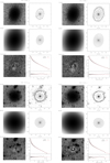 |
Fig. A.1. As in Fig. 5. Summary of the surface photometric analysis of KIG 378 (top panels) and KIG 412 (bottom panels). In both bands we show the B+D best-fit models. We show 20 isophote levels, between 500 and 2 σ of the sky level, for the original and model images. |
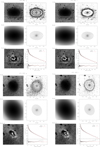 |
Fig. A.2. As in Fig. 5. Summary of the surface photometric analysis of KIG 481 (top panels) and KIG 490 (bottom panels). In both bands the B+D best-fit models are shown. The KIG 481 image shows the gap in the 4K CCD and a dust feature that was not removed by the flat-fielding. We show 20 isophote levels, between 500 and 2σ of the sky level, for the original and model images. |
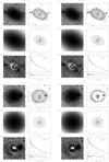 |
Fig. A.3. As in Fig. 5. Summary of the surface photometric analysis of KIG 517 (top panels) and KIG 578 (bottom panels). The B+D and Sérsic best-fit models are shown for KIG 517 and KIG 578, respectively. We show 20 isophote levels, between 500 and 2σ of the sky level, for the original and model images. |
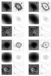 |
Fig. A.4. As in Fig. 5. Summary of the surface photometric analysis of KIG 595 (top panels) and KIG 599 (bottom panels). In both bands we show the B+D models. We show 20 isophote levels, between 500 and 2σ of the sky level, for the original and model images. |
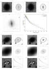 |
Fig. A.5. Summary of the surface photometric analysis of KIG 620 (top panels). Deep g and r images are shown, with isophote contours down to the 2σ level of the sky. Middle panels: the right g image enhances the central part of KIG 620, showing the ring structure, and the left panel shows the g and r light profiles. Bottom panels: as in Fig. 5, but for KIG 636. The B+D model is shown. We show 20 isophote levels, between 500 and 2 σ of the sky level, for the original and model images. |
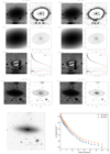 |
Fig. A.6. As in Fig. 5. Summary of the surface photometric analysis of KIG 637 (top panels). In both bands we show the B+D models. The image of KIG 637 shows the gap in the 4K CCD. The corona of the bright star HD 238370, south of the galaxy nucleus, extends across the entire galaxy and strongly affects the photometric measures. We show 20 isophote levels, between 500 and 2σ of the sky level, for the original and model images. Summary of the surface photometric analysis of KIG 644 (middle and bottom panels). Deep g and r images are shown with isophote contours down to the 2σ level of the sky. The right r image enhances the central part of KIG 644, showing the ring and the lens structures; the left panel shows the g and r light profiles. |
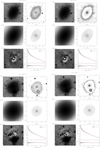 |
Fig. A.7. As in Fig. 5. Summary of the surface photometric analysis of KIG 670 (top panels) and KIG 685 (bottom panels). In both bands we show the B+D models. We show 20 isophote levels, between 500 and 2σ of the sky level, for the original and model images. |
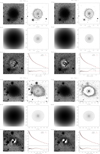 |
Fig. A.8. As in Fig. 5. Summary of the surface photometric analysis of KIG 705 (top panels) and KIG 722 (bottom panels). In both bands for KIG 722 we show the Sérsic models. We show 20 isophote levels, between 500 and 2σ of the sky level, for the original and model images. |
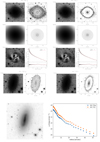 |
Fig. A.9. As in Fig. 5. Summary of the surface photometric analysis of KIG 732 (top panels). We show the B+D model. We show 20 isophote levels, between 500 and 2σ of the sky level, for the original and model images. Summary of the surface photometric analysis of KIG 733 (middle panels). Deep g and r images are shown with isophote contours down to the 2σ level of the sky. Bottom panels: the right r image enhances the central part of KIG 733, showing the ring and the arm-like structure, and the left panel shows the g and r light profiles. |
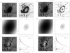 |
Fig. A.10. As in Fig. 5. Summary of the surface photometric analysis of KIG 841. In both bands we show the B+D models. We show 20 isophote levels, between 500 and 2σ of the sky level, for the original and model images. The gap in the 4K CCD and a dust feature on the CCD that is not removed by the flat-fielding are visible. |
All Tables
KIG photometric data from the adopted Sérsic and B+D best-fit models and morphological notes.
All Figures
|
Fig. 1. Comparison between the three classifications into morphological type provided in Table 1. The dashed red rectangle encloses iETGs (T ≤ 0) in the RC3 classification. Comparisons are made between HyperLeda vs. Buta et al. (2019) (top panel), HyperLeda vs. Fernandez-Lorenzo et al. (2012) (middle panel), and Buta et al. (2019) vs. Fernandez-Lorenzo et al. (2012) (bottom panel). |
| In the text | |
|
Fig. 2. Degree of isolation of the observed sample (green circles) over-plotted on all iETGs (red circles) in the AMIGA sample. According to Verley et al. (2007a), the horizontal and vertical dashed lines enclose the fiducial range of isolated galaxies in the AMIGA sample. |
| In the text | |
|
Fig. 3. Top panel: 2D map of the PSF FWHM variation across the g -band FOV of KIG 264. Middle panel: FWHM measured along the x-axis (RA) and along the y-axis (Decl., bottom panel) of this frame. The vertical red line marks the position of KIG 264. |
| In the text | |
|
Fig. 4. PSF in KIG 264 in the g band. The 2D PSF is best fitted with a composite model (solid line) combining three Gaussians plus an exponential. The adopted PSF has been generated from a set of stars (star 6 is shown) close to the galaxy. The seeing correction is extrapolated up to the galaxy outskirts (see the discussion in Rampazzo et al. 2019, and references therein). A masked star is visible on the NW side of the field. |
| In the text | |
|
Fig. 5. Summary of the g− (left panels) and r− (right panels) band surface photometry of KIG 264. The adopted masks of the foreground and background objects are not shown. North is up, and east is to the left. The right panels provide from top to bottom (left) the original image, the best-fit model image, and the image of residuals after model subtraction for the g band. (right) Isophotal contours of the image, of the model, and of the azimuthal light profile. For clarity, only the model (red line) is over-plotted on the azimuthal light profile, and the (O–C) residuals are shown. Table 4 reports the model parameters. We show 20 isophote levels, between 500 and 2 σ of the sky level (μg = 21.6 ± 0.02 and 26.9 ± 0.34 mag arcsec−2 and μr = 21.0 ± 0.02 and 26.6 ± 0.29 mag arcsec−2), for the original and model images. The same panels are shown for the r-band photometry. KIG 264 reveals ripples and tail at the NW side of the galaxy body and a shell system in the outskirts. These features are revealed in both the g and r images above 2σ of the sky level and in the light profiles, starting at ≈30″. |
| In the text | |
|
Fig. 6. Comparison between our integrated magnitudes in g and r bands with the SDSS DR16 values reported in Table 2. The solid lines show our errors. KIG 637 is not plotted because the magnitudes are strongly influenced by the nearby bright star HD238370 (see Sect. 4.2). |
| In the text | |
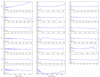 |
Fig. 7. Galaxy (g − r) colour profiles. Single profiles are presented and discussed in Sect. 4.2. |
| In the text | |
|
Fig. 8. (g − r) colour profiles in kpc (using the galaxy distance provided in Table 1). Colour profiles have been subdivided into three classes according to their behaviour outside the seeing-dominated area: galaxies with colour profiles become redder with radius (top panel), flat colour profiles (middle panel), and colour profiles with a peculiar behaviour or that become bluer in the outskirts (bottom panel). |
| In the text | |
|
Fig. 9. Distribution of B/T in the g (top panel) and r bands. The average B/T values is 0.66 in both bands. |
| In the text | |
|
Fig. 10. UV-optical CMD of iETGs. In the Mr vs. (NUV-r) plane we plot the Wyder et al. (2007) fits to the red sequence (magenta dots and dotted line) and to the blue cloud (cyan dots and dotted line). iETGs with a shell system are indicated with orange dots. KIG 722 is missing from the iETGs sample because no NUV measures are available. The dotted vertical lines provide an indication of the green valley crossing time as a function of the galaxy luminosity (see text). The horizontal error bar accounts for a distance uncertainty of 10%. The vertical error bar accounts for the NUV ZP uncertainty, 0.15 mag (Bai et al. 2015). |
| In the text | |
|
Fig. A.1. As in Fig. 5. Summary of the surface photometric analysis of KIG 378 (top panels) and KIG 412 (bottom panels). In both bands we show the B+D best-fit models. We show 20 isophote levels, between 500 and 2 σ of the sky level, for the original and model images. |
| In the text | |
|
Fig. A.2. As in Fig. 5. Summary of the surface photometric analysis of KIG 481 (top panels) and KIG 490 (bottom panels). In both bands the B+D best-fit models are shown. The KIG 481 image shows the gap in the 4K CCD and a dust feature that was not removed by the flat-fielding. We show 20 isophote levels, between 500 and 2σ of the sky level, for the original and model images. |
| In the text | |
|
Fig. A.3. As in Fig. 5. Summary of the surface photometric analysis of KIG 517 (top panels) and KIG 578 (bottom panels). The B+D and Sérsic best-fit models are shown for KIG 517 and KIG 578, respectively. We show 20 isophote levels, between 500 and 2σ of the sky level, for the original and model images. |
| In the text | |
|
Fig. A.4. As in Fig. 5. Summary of the surface photometric analysis of KIG 595 (top panels) and KIG 599 (bottom panels). In both bands we show the B+D models. We show 20 isophote levels, between 500 and 2σ of the sky level, for the original and model images. |
| In the text | |
|
Fig. A.5. Summary of the surface photometric analysis of KIG 620 (top panels). Deep g and r images are shown, with isophote contours down to the 2σ level of the sky. Middle panels: the right g image enhances the central part of KIG 620, showing the ring structure, and the left panel shows the g and r light profiles. Bottom panels: as in Fig. 5, but for KIG 636. The B+D model is shown. We show 20 isophote levels, between 500 and 2 σ of the sky level, for the original and model images. |
| In the text | |
|
Fig. A.6. As in Fig. 5. Summary of the surface photometric analysis of KIG 637 (top panels). In both bands we show the B+D models. The image of KIG 637 shows the gap in the 4K CCD. The corona of the bright star HD 238370, south of the galaxy nucleus, extends across the entire galaxy and strongly affects the photometric measures. We show 20 isophote levels, between 500 and 2σ of the sky level, for the original and model images. Summary of the surface photometric analysis of KIG 644 (middle and bottom panels). Deep g and r images are shown with isophote contours down to the 2σ level of the sky. The right r image enhances the central part of KIG 644, showing the ring and the lens structures; the left panel shows the g and r light profiles. |
| In the text | |
|
Fig. A.7. As in Fig. 5. Summary of the surface photometric analysis of KIG 670 (top panels) and KIG 685 (bottom panels). In both bands we show the B+D models. We show 20 isophote levels, between 500 and 2σ of the sky level, for the original and model images. |
| In the text | |
|
Fig. A.8. As in Fig. 5. Summary of the surface photometric analysis of KIG 705 (top panels) and KIG 722 (bottom panels). In both bands for KIG 722 we show the Sérsic models. We show 20 isophote levels, between 500 and 2σ of the sky level, for the original and model images. |
| In the text | |
|
Fig. A.9. As in Fig. 5. Summary of the surface photometric analysis of KIG 732 (top panels). We show the B+D model. We show 20 isophote levels, between 500 and 2σ of the sky level, for the original and model images. Summary of the surface photometric analysis of KIG 733 (middle panels). Deep g and r images are shown with isophote contours down to the 2σ level of the sky. Bottom panels: the right r image enhances the central part of KIG 733, showing the ring and the arm-like structure, and the left panel shows the g and r light profiles. |
| In the text | |
|
Fig. A.10. As in Fig. 5. Summary of the surface photometric analysis of KIG 841. In both bands we show the B+D models. We show 20 isophote levels, between 500 and 2σ of the sky level, for the original and model images. The gap in the 4K CCD and a dust feature on the CCD that is not removed by the flat-fielding are visible. |
| In the text | |
Current usage metrics show cumulative count of Article Views (full-text article views including HTML views, PDF and ePub downloads, according to the available data) and Abstracts Views on Vision4Press platform.
Data correspond to usage on the plateform after 2015. The current usage metrics is available 48-96 hours after online publication and is updated daily on week days.
Initial download of the metrics may take a while.