| Issue |
A&A
Volume 640, August 2020
|
|
|---|---|---|
| Article Number | A18 | |
| Number of page(s) | 19 | |
| Section | Astrophysical processes | |
| DOI | https://doi.org/10.1051/0004-6361/202037539 | |
| Published online | 31 July 2020 | |
A unified accretion-ejection paradigm for black hole X-ray binaries
V. Low-frequency quasi-periodic oscillations
1
Villanova University, Department of Physics, Villanova, PA 19085, USA
e-mail: This email address is being protected from spambots. You need JavaScript enabled to view it.
, This email address is being protected from spambots. You need JavaScript enabled to view it.
2
AIM, CEA, CNRS, Université Paris-Saclay, Université Paris Diderot, Sorbonne Paris Cité, 91191 Gif-sur-Yvette, France
3
Univ. Grenoble Alpes, CNRS, IPAG, 38000 Grenoble, France
4
IRAP, Université de Toulouse, CNRS, UPS, CNES, Toulouse, France
Received:
20
January
2020
Accepted:
20
May
2020
Abstract
Context. We proposed in paper I that the spectral evolution of transient X-ray binaries (XrB) is due to an interplay between two flows: a standard accretion disk (SAD) in the outer parts and a jet-emitting disk (JED) in the inner parts. We showed in papers II, III, and IV that the spectral evolution in X-ray and radio during the 2010–2011 outburst of GX 339-4 can be recovered. However, the observed variability in X-ray was never addressed in this framework.
Aims. We investigate the presence of low frequency quasi-periodic oscillations (LFQPOs) during an X-ray outburst, and address the possible correlation between the frequencies of these LFQPOs and the transition radius between the two flows, rJ.
Methods. We select X-ray and radio data that correspond to 3 outbursts of GX 339-4. We use the method detailed in Paper IV to obtain the best parameters rJ(t) and ṁin(t) for each outburst. We also independently search for X-ray QPOs in each selected spectra and compare the QPO frequency to the Kepler and epicyclic frequencies of the flow in rJ.
Results. We successfully reproduce the correlated evolution of the X-ray spectra and the radio emission for 3 different activity cycles of GX 339-4. We use a unique normalisation factor for the radio emission, f∼R. We also report the detection of 7 new LFQPOs (3 Type B, and 4 Type C), to go along with the ones previously reported in the literature. We show that the frequency of Type C QPOs can be linked to the dynamical JED-SAD transition radius rJ, rather than to the optically thin-thick transition radius in the disk. The scaling factor q such that νQPO ≃ νK(rJ)/q is q ≃ 70 − 130, a factor consistent during the 4 cycles, and similar to previous studies.
Conclusions. The JED-SAD hybrid disk configuration not only provides a successful paradigm allowing us to describe XrB cycles, but also matches the evolution of QPO frequencies. Type C QPOs provide an indirect way to probe the JED-SAD transition radius, where an undetermined process produces secular variability. The demonstrated relation between the transition radius links Type C QPOs to the transition between two different flows, effectively tying it to the inner magnetized structure, i.e., the jets. This direct connection between the jets’ (accretion-ejection) structure and the process responsible for Type C QPOs, if confirmed, could naturally explain their puzzling multi-wavelength behavior.
Key words: black hole physics / accretion / accretion disks / magnetohydrodynamics (MHD) / ISM: jets and outflows / X-rays: binaries / stars: individual: GX 339-4
© ESO 2020
1. Introduction
The generic behavior of X-ray binaries is now well captured in the literature (e.g., Dunn et al. 2010). These systems spend most of their life in a quiescent and barely detectable state, sometimes for years, before undergoing sudden X-ray outbursts lasting weeks/months. These outbursts are accompanied by spectral changes following a similar pattern for most objects. Starting from quiescence, the total luminosity increases in both X-ray and radio bands. Radio flux is detectable, and the X-ray spectrum peaks above 10 keV: this state is called the hard state. Systems remain in this state over several orders of magnitude in X-ray and radio luminosities. At some point, the radio flux vanishes and the X-ray spectrum then peaks around 1 keV: this is the soft state1. Once in the soft-state, the flux eventually decreases until the source transitions back to the hard state, along with the reappearance of detectable radio fluxes. In the so-called hardness-intensity diagram (Körding et al. 2006), this behavior produces the archetypal “q”-cycle of X-ray binaries (for a review, see e.g., Dunn et al. 2010). To date, there is no consensus explanation for these cycles (Remillard & McClintock 2006; Yuan & Narayan 2014). It is however very likely that the X-ray spectral changes are due to variations in the inner accretion flow structure (see e.g., Done et al. 2007, and references therein).
To explain this behavior, Esin et al. (1997)2 envision the interplay between an outer standard accretion disk (SAD; Shakura & Sunyaev 1973) and an inner advection-dominated flow (Ichimaru 1977; Rees et al. 1982; Narayan & Yi 1994). However, although the presence of a standard accretion disk in the outer regions seems inevitable (Done et al. 2007), the inner advection-dominated flow structure remains uncertain. The many scenarios following Esin et al. (1997) notably fail to explain the radio (non-)detections. Radio detections are commonly interpreted as persistent self-collimated jets (Blandford & Königl 1979; Mirabel et al. 1992), whereas non-detections in radio are the result of jet quenching (Corbel et al. 2004; Fender et al. 2004, see however Drappeau et al. 2017, for an alternative view). Ignoring the formation and quenching of jets leaves important observational diagnostics unexplained (for recent discussions, see Yuan & Narayan 2014; Marcel et al. 2018b).
A framework addressing the full accretion-ejection phenomenon was proposed and progressively elaborated in a series of papers. Ferreira et al. (2006, hereafter Paper I), proposed that the disk be threaded by a large-scale vertical magnetic field Bz, build up mostly by accumulation from the outer disk regions. In this configuration the magnetization  , with P the total (gas plus radiation) pressure at the disk mid-plane, increases inwardly to reach an expected threshold value μ ∼ 0.5. A jet-emitting disk (JED) emerges. While jet-emitting disks can nicely reproduce bright hard states at luminosity levels never achieved in any other accretion model (Yuan & Narayan 2014), a sole JED configuration cannot explain the spectral cycles as those of GX 339-4 (Marcel et al. 2018b, hereafter Paper II). When transitioning to the soft state, the system needs to not only emit a sufficiently soft spectrum, but also to fully quench its jets. Similarly to Esin et al. (1997), we imagined the existence of a transition at some radius rJ, from an inner JED to an outer SAD, as already proposed in Paper I. We note that very recent numerical simulations naturally show such a magnetic field distribution: μ ≳ 0.1 in the inner region and μ ≪ 1 in the outer region (Scepi et al. 2019; Liska et al. 2019). In Marcel et al. (2018a, hereafter Paper III), we showed that the observed domain in X-ray luminosities and hardness ratios during a standard XrB cycles can be covered by changing rJ and the inner accretion rate ṁ(risco) = ṁin. Along with these X-ray signatures, JED-SAD configurations naturally account for the radio emission whenever it is observed. As an illustration, we successfully reproduced five canonical spectral states (X-ray+radio) typically observed along a cycle. In Marcel et al. (2019, hereafter Paper IV), we reproduced independently each step of the spectral evolution of the 2010–2011 outburst from GX 339-4, using 35 observed radio fluxes and 297 X-ray spectral fits from Clavel et al. (2016). We showed that a smooth evolution in disk accretion rate and transition radius can simultaneously reproduce the behavior of GX 339-4 in the X-ray and radio bands. For the first time, a time-evolution of physical parameters reproduced the behavior of a given X-ray binary in multiple spectral bands. However, there are multiple open questions remaining, such as the origin of timing properties in the JED-SAD paradigm (see Sect. 4.3 in Paper IV).
In particular, quasi-periodic oscillations (QPO) of the X-ray flux are ubiquitous features of XrBs (see e.g., Miyamoto & Matsuoka 1977; Samimi et al. 1979; Zhang 2013, and references therein). When studying the power density spectra (PDS) in the Fourier space (van der Klis 1989), peaks are observed at varying frequencies and with varying width (Miyamoto et al. 1991; Homan et al. 2005). These peaks, called QPOs, have been detected in a very wide number of XrBs so far (Zhang 2013). They are observed to evolve with the X-ray spectral shape, but remain a considerable unknown of the X-ray binaries’ behavior (see Motta 2016, for a recent review). They cover a wide range of frequencies up to kHz, but we focus in this paper on the low frequency (0.1 − 10 Hz) QPOs. There are three types: A, B, and C, defined using their frequencies, width, broad-band noise, and amplitude (Casella et al. 2005). Type A are characterized by a weak and broad peak around 6 − 8 Hz, the absence of brand-band noise, and are found on the soft side of state transitions (hard ↔ soft). They are the rarest type of low-frequency quasi-periodic oscillations. Type B are characterized by an intermediate and narrow peak, varying between 1 and 6 Hz, the absence of brand-band noise, and are detected during the soft-intermediate state. Their detection is much more common than Type A, but most detected quasi-periodic oscillations are of the next type. Type C are characterized by a strong and very narrow peak, varying between 0.1 and 10 Hz, a very important brand-band noise, and are detected during the hard and hard-intermediate states. Type C are, by far, the most studied type of quasi-periodic oscillation in the literature. We discern three key features of Type C LFQPOs from observations (Remillard & McClintock 2006; Motta 2016). First, the stability and persistence of the frequencies suggest that Type C LFQPOs originate in the accretion flow itself. Second, they vary significantly in frequency, especially during state transitions, i.e., when the accretion flow structure is expected to change the most. Third, their root mean square (rms) amplitude is strongest in the hard X-ray band, which indicates a connection with the power-law component of the X-ray spectrum. Guided by these important properties, LFQPOs are commonly associated with the inner hot flow (see Sect. 4.4.1 in McClintock & Remillard 2006). Indeed, a link between the LFQPOs and the outer radius of the inner flow was observed in very early works (e.g., Muno et al. 1999; Sobczak et al. 2000; Trudolyubov et al. 1999; Revnivtsev et al. 2000; Rodriguez et al. 2002, 2004).
In this paper, we intend to investigate a possible correlation between all types of QPO frequencies and the jet-emitting disk parameters. We present in Sect. 2 the selected data sets in both X-ray and radio bands, our methodology to obtain estimates of rJ and ṁin, as well as the fitting results applying the method from Paper IV. Later in the same section, we also present the methodology and results concerning the LFQPOs, and compare it to the literature. In Sect. 3, we investigate the link between the frequency of the QPOs obtained/selected and the accretion flow structure. We finish by some discussions, conclusions, and upcoming work in Sect. 4.
2. Multi-spectral reproduction of outbursts
We summarize in this section the procedure we followed to reproduce the observed spectra within our theoretical framework. The caveats, statistical/systematic, and limitations of the results were extensively discussed in Paper IV, and we will only develop the major outcomes here.
2.1. Data selection
We selected the archetypal object GX 339-4 to investigate the capability of our theoretical model to reproduce X-ray binaries in outbursts. We chose this object due to both its historic place and its short recurrence time of outbursts, once every two years on average (Tetarenko et al. 2016). We used two different data sets: X-ray spectra and radio fluxes. In X-ray, we selected the 3 − 40 keV RXTE/PCA data reduced and fitted by Clavel et al. (2016). In radio, we used results obtained with the Australia Telescope Compact Array (ATCA, Corbel et al. 2013a,b).
We show in Fig. 1 the unabsorbed light curves3 of the two additive models from Clavel et al. (2016) fits: the power-law (dark violet) and disk (light cyan). We show in yellow markers on the lower X-axis the dates when LFQPOs were detected by previous studies (Motta et al. 2011; Nandi et al. 2012; Gao et al. 2014; Zhang et al. 2017), and in red markers on the upper X-axis when the source was observed and detected in radio (Corbel et al. 2013b). One can already note that the coverage of radio observations is extremely diverse: while the 2010–2011 outburst is widely covered, the 2002–2003 region was only observed at two very different stages. Four zones are highlighted in gray in this figure, defining major/full outbursts. The exact dates of these events are reported in Table 1.
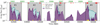 |
Fig. 1. RTXE/PCA lightcurves of GX 339-4 in the 3 − 200 keV energy band from 2002 to 2011 (see upper X-axis). In filled colors, the power-law (violet), and disk (cyan) unabsorbed fluxes from the Clavel et al. (2016) fits. In gray, the area corresponding to the 4 complete outbursts (#1, #2, #3, #4). Red lines at the top correspond to dates when steady radio fluxes were observed with the Australia telescope compact array (ATCA) at 9 GHz (Corbel et al. 2013a,b). Yellow lines at the bottom show previous detections of quasi-periodic oscillations (QPO, Motta et al. 2011; Nandi et al. 2012; Gao et al. 2014; Zhang et al. 2017). |
Four full cycles from GX 339-4 during the 2001–2011 decade and their associated number of observations in X-rays and radio.
Outburst #4 is the 2010–2011 outburst previously reproduced in Paper IV, whereas outbursts #1, #2, and #3 correspond to 2002–2003, 2004–2005, and 2006–2007, respectively. One can note that all these outbursts follow the standard trend described in introduction: increase in luminosity, appearance of a disk component (in cyan), decrease in luminosity. There are also hard-only (failed) outbursts, i.e., luminosity increases in which the disk component is never detected (see e.g., 2006 and 2008–2009). We define spectral states solely based on the shape of the continuum (i.e., no timing or radio properties, see Sect. 2.2 in Paper IV).
2.2. Methodology
We chose the following global parameters for GX 339-4:
-
Source distance d ≃ 8 ± 1 kpc (Hynes et al. 2004; Zdziarski et al. 2004; Parker et al. 2016),
-
Black hole mass m = M/M⊙ = 5.8, with M⊙ the mass of the Sun (Hynes et al. 2003; Muñoz-Darias et al. 2008; Parker et al. 2016; Heida et al. 2017),
-
Disk innermost stable circular orbit4risco = rin = Rin/Rg = 2 (i.e., spin 0.94, Reis et al. 2008; Miller et al. 2008; García et al. 2015), with Rg = GM/c2 the gravitational radius, G the gravitational constant, c the speed of light, and M the black hole mass,
In this work, the disk accretion rate is normalized with respect to the Eddington rate ṁ = Ṁ/ṀEdd = Ṁc2/LEdd (Eddington 1926). We note that this definition of ṁ does not include any accretion efficiency. In practice, we will mostly use the accretion rate at the innermost disk radius ṁin = ṁ(risco), and we recall that we assume ṁ(r) = ṁin(r/risco)0.01 in the jet-emitting disk region (Paper II).
We simulate a large set of parameters rJ ∈ [risco = 2, 103] and ṁin ∈ [10−3, 10]. For each pair (rJ,ṁin), we compute the thermal balance of the hybrid disk configuration, and its associated global spectrum self-consistently. We then fit each simulated spectrum with the same spectral model components as those used for the spectral analysis of the observations. As a consequence, the simulated parameters of the fits can be directly compared to the observational parameters, i.e., those from observational fits (Clavel et al. 2016). Among these parameters, we select: the 3 − 200 keV luminosity L3 − 200, the power-law fraction PLf = Lpl/L3 − 200 with Lpl the power-law flux in the 3 − 200 keV energy band, and the power-law photon index Γ. This selection provides us with 3 constraints for any given simulated X-ray spectrum to reproduce. Additionally, we estimate for any couple (rJ,ṁin) the synchrotron emission radiated by the jet using a self-similar approach (Blandford & Königl 1979; Heinz & Sunyaev 2003, Appendix A in Paper III, Sect. 3.2.2 in Paper IV). We can thus uniquely link the steady radio flux observed to the accretion flow structure,
 (1)
(1)
with  a scaling factor, found to best fit observations at
  for outburst #4, and FEdd = LEdd/(νR4πd2) the Eddington flux at νR = 9 Hz received at a distance d (Paper IV).
We tested different minimization procedures in Paper IV and selected the most promising for the 2010–2011 outburst. For any given observation, our procedure uses variable weights to minimize the differences with the 4 constraints/parameters: the first three in X-rays (L3 − 200, PLf, Γ), and the last one in radio (FR). In this paper, we thus use the exact same procedure on the other 3 selected outbursts. The procedure searches for the pair of parameters (rJ,ṁin) that minimizes, for each individual observation, the following function:
![Mathematical equation: $$ \begin{aligned} \zeta _{X+R} =&\frac{ \left| \log \left[ L_{3-200} / L_{3-200}^\mathrm{obs} \right] \right| }{\alpha _{\rm flux}} + \frac{ \left| \log \left[ \mathrm{PLf} / \mathrm{PLf}_{\rm obs} \right] \right| }{\alpha _{\mathrm{PLf}}} \nonumber \\& + \frac{ \left| \Gamma - \Gamma ^\mathrm{obs} \right| }{\alpha _{\Gamma }} + \frac{ \left| \log \left[ F_R / F_R^\mathrm{obs} \right] \right| }{\alpha _{R}} \end{aligned} $$](/articles/aa/full_html/2020/08/aa37539-20/aa37539-20-eq6.gif) (2)
(2)
with  , PLfobs, Γobs, and
  the observational constraints (Corbel et al. 2013a,b; Clavel et al. 2016). The selected weights are αΓ = 2 − 6log10 (PLf), αflux = αPLf = 1, and αR = 5, see Eqs. (1) and (4) in Paper IV. When no radio flux can be estimated (i.e., during the entire soft and soft intermediate states), we use 1/αR = 0 (see Sect. 4.1 in Paper IV).
2.3. Results
We use this procedure to derive the best (rJ,ṁin) for all observations in the 4 outbursts. We show these results in Fig. 2 for outbursts #1 and #2, and Fig. 3 for outbursts #3 and #45. Remarkably here, the same factor  can effectively be used to reproduce all four outbursts. This parameter is a combination of many different physical properties (e.g., Bz or risco, see Papers III, IV), but it is a simple proxy for the jet radiative efficiency. It is thus noteworthy that
  could remain constant all along the evolution of the 4 outbursts, i.e., after 3 jets quenching/building.
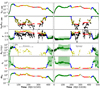 |
Fig. 2. Observation and model parameters for cycles #1 (2002–2003, left) and #2 (2004–2005, right). From top to bottom: X-ray flux and power-law fraction in the 3 − 200 keV range, power-law index, 9 GHz radio flux, transition radius rJ, and inner accretion rate ṁin (at ISCO). For the first 4 panels, i.e., the constraints, black squares are observations. Each figure uses the same color-code: green upper- (lower-) triangles for the rising (decaying) hard, blue circles for hard-intermediate, yellow crosses for soft-intermediate, and red crosses for soft-states. Additionally, in the state-associated colors we draw the 5% and 10% confidence intervals (i.e., 5% and 10% bigger ζX + R, see Paper IV). Double arrows are drawn when radio emission was also observed but has been interpreted as radio flares or interactions with the interstellar medium (Corbel et al., in prep.). |
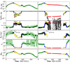 |
Fig. 3. Observation and model parameters for cycles #3 (2006–2007, left) and #4 (2010–2011, right). From top to bottom: X-ray flux and power-law fraction in the 3 − 200 keV range, power-law index, 9 GHz radio flux, transition radius rJ, and inner accretion rate ṁin (at ISCO). For the first 4 panels, i.e., the constraints, black squares are observations. Each figure uses the same color-code: green upper- (lower-) triangles for the rising (decaying) hard, blue circles for hard-intermediate, yellow crosses for soft-intermediate, and red crosses for soft-states. Additionally, in the state-associated colors we draw the 5% and 10% confidence intervals (i.e., 5% and 10% bigger ζX + R, see Paper IV). Double arrows are drawn when radio emission was also observed but has been interpreted as radio flares or interactions with the interstellar medium (Corbel et al., in prep.). |
In the hard and hard-intermediate cases, both the X-ray flux and the power-law fractions (top 2 panels) are very well reproduced in all 4 outbursts. The theoretical power-law index during these 2 states, i.e., when the power-law is dominant, follows the observed one very well. The model also reproduces the radio flux extremely well when present, but occasionally at the expense of matching Γ. See for example the first 50 days of outburst #2, when the radio constraints are associated with small inaccuracies in Γ. However, the maximum difference is |Γth − Γobs| ≃ 0.1, i.e., only twice the average error ΔΓobs = 0.05 in hard and hard-intermediate states in observational fits from Clavel et al. (2016). As we showed in Papers III and IV, these differences can be corrected by local/physical parameters of our model (such as the illumination fraction) or by including reflection in the theoretical model. We would like to point out that reflection is not expected to have a huge impact: we compare the theoretical continuum to the observed continuum extracted from observational fits that were performed using multiple reflection models (Clavel et al. 2016). We also recall that the predicted radio flux from Eq. (1) is a very simple and first order approximation.
Modeling is more complex in the case of soft-intermediate and soft states. In disk-dominated states, the hard part of the X-ray spectrum is dominated by the so-called hard tail, a steep power-law (Γ ∼ 2.5) with no clear high-energy cut-off (see Remillard & McClintock 2006). There is no consensus about the physical origin of this component, and we thus decide to use a proxy: we add a steep power-law with index 2.5 to represent 10% of the 3 − 20 keV flux (Paper III). Although a 10% hard tail was ideal in outburst #4, a different level could in principle be necessary in the other 3 outbursts, and the hard tail proxy might vary with time. Because of this proxy, the transition from soft-intermediate to soft states is not clear-cut: some of the states classified as soft could be soft-intermediate, and vice versa. While one often uses timing properties to disentangle between these two states, we wish to only use the X-ray continuum here. As one can see in the large statistical error-bars in the fits from Clavel et al. (2016), this is not a major issue for the minimizing procedure since both these states are disk-dominated and Γ is often unreliable. However, an important aspect of our model is its ability to link radio and X-ray fluxes, a unique characteristic of disk-driven ejections (Blandford & Payne 1982; Ferreira 1997, and references therein). Minor state differences between the soft and soft-intermediate states could then translate into major dynamical differences; See for example the soft-intermediate phase of outburst #3, when radio flux is predicted by the model but was not observed. It is also possible that the jet is not fully self-similar for small values of transition radius rJ ≳ risco (i.e., during spectrally soft states; see Sect. 3.2.2 in Paper IV). In other words, even if a JED is present in the inner regions during the soft-intermediate states, and thus ejections are produced, we do not expect the jet production to be correctly reproduced by our approach. For this reason, although emission is predicted but not observed, we do not believe this represents a fundamental issue with the model.
2.4. Timing properties
RXTE/PCA data were already treated in the past in (at least) 4 comprehensive studies: Motta et al. (2011), Nandi et al. (2012), Gao et al. (2014), and Zhang et al. (2017). Since we found discrepancies among previous QPO (non-)detections (see e.g., obsID 95409-01-17-02), we decided to perform our own analysis to get a consistent data set. In order to address this issue in a model-independent way, the QPO types are solely defined using the PDS fitting results of the following procedure (i.e., no time lags or spectral states).
2.4.1. Methodology
To analyze the timing, we consider GoodXenon, Event, and Binned data modes from all RXTE/PCA archival observations of GX 339-4. We reduce the data using the version 6.24 of the HEASOFT. We follow standard procedures6 to filter bad time intervals, and extract lightcurves with binsize of 2−10 s and 2−7 s in three different energy bands to probe different emission regions: spectral channels 6 − 13, 14 − 47, and 6 − 47 (energy bands 2.87 − 6.12 keV, 6.12 − 19.78 keV, and 2.87 − 19.78 keV, PCA calibration epoch 5). We then extract power spectra from the three light curves with the powspec tool, and convert them into XSPEC readable files in order to ease the fits. We use version 12.10.0c of XSPEC for the PDS fittings.
We use a semi-automatic iterative process to fit the PDS with pyXSPEC. To represent the white noise, we first fit the high-frequency part of the 2−10 s binsized PDS with a constant (i.e., a power-law slope of 0). The high-frequency part corresponds to the 80 − 512 Hz. Leaving the normalization free to vary allows one to precisely estimate the dead time affected level of white noise (see e.g., Varnière & Rodriguez 2018). For the power spectra extracted with the 2−7 binsize, the maximum frequency is 64 Hz, thus we fit the white noise with a frozen flat power-law of normalization 2.
We then freeze the parameters of this component and consider the PDS over the entire frequency range. If the fit is valid (i.e.,  ), no additional component is needed and we do not consider the observation further. If the PDS diverges from pure white noise, we first add a zero-centered Lorentzian initialized with all its parameters left free. If the fit statistic is poor (
 ) after the initial fit, we iterate the process by adding a new Lorentzian at the frequency of the largest residuals. This iterative process is repeated up to 4 times, i.e., 5 total Lorentzians (broad or narrow). When a good fit is achieved, we calculate the coherence factor Q = f/Δf of each Lorentzian, where f is the centroid frequency and Δf the width. We identify a Lorentzian as a QPO if its coherence factor is Q > 2 with a significance > 5σ. We note that 5 Lorentzians are enough for all the fits to converge in this paper, and among all the fitted Lorentzians, about 2% of them are detected as QPOs. The QPO type is derived only from its coherence factor (A or B/C) and the presence of source broad band noise (B or C).
2.4.2. Results
We have applied this method to all RXTE/PCA observations of GX 339-4. We found a total of 84, 107, and 93 QPOs in the 2.87 − 6.12 keV, 6.12 − 19.78 keV, and 2.87 − 19.78 keV band, respectively. We found no significant differences in the QPO frequency7 between the different energy channels and will then present the results in the largest energy band (2.78 − 19.78 keV). We summarize these numbers in Table 2, as well as those obtained in other works using the same X-ray data. We note that Motta et al. (2011) and Nandi et al. (2012) searched for LFQPOs in the 2 − 15 keV range, Gao et al. (2014) in the 2 − 24 keV range, and Zhang et al. (2017) in the 2 − 60 keV range, explaining the potential differences (see Appendix A). The entire list of the detected LFQPOs using these data can be found in Table C.1, as well as the list of new different ones in Table C.2.
Number of reported (fundamental) LFQPOs in GX 339-4 using the RXTE/PCA observations.
We plot the observed low frequency quasi-periodic oscillations in the disk fraction luminosity diagrams (DFLDs) at the bottom of Fig. 4. As expected, Type C QPOs are detected in the hard state and during the beginning of transitions, Type B mainly during transitions, and Type A particularly at the end of the hard-to-soft transition. While this is usually a byproduct of the definition of each type, we recall that the QPO types (A, B, or C) and the spectral states (hard, hard-intermediate, soft-intermediate, or soft) are defined using independent methods in this study. We show the time evolution of the QPO frequency in Fig. 5.
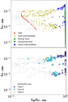 |
Fig. 4. DFLDs showing the distribution of states (top) and observed LFQPOs (bottom). Top panel: states are shown in the same color-code as in Figs. 2 and 3 (see legend). Bottom panel: in different colors, position where QPOs were identified (see legend). Light gray squares in background are observations from Clavel et al. (2016). |
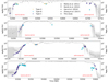 |
Fig. 5. Co-evolution of the observed QPO frequency νQPO and the Kepler rotation frequency νK(rJ) for the 4 different outbursts, showing both hard-to-soft and soft-to-hard transitions (see red annotations). On the left Y-axis, the Kepler frequency at the transition radius, νK(rJ), and the 5% and 10% confidence intervals. On the right Y-axis, the observed QPO frequency, νQPO. Different markers are used to disentangle the different works: Motta et al. (2011) in upper-triangles, Nandi et al. (2012) in lower-triangles, Gao et al. (2014) in crosses, Zhang et al. (2017) in plus signs, and new detections in circle markers (see text). We also use different colors for the different types of QPOs (see legend). |
3. LFQPOs and the accretion flow
3.1. LFQPOs and the accretion flow parameters
Multiple authors have suggested in the past a possible correlation between QPO frequency and the disk flux or accretion rate (see e.g., Trudolyubov et al. 1999; Revnivtsev et al. 2000; Sobczak et al. 2000). However, such a correlation works only on a short range of QPO frequencies, and we will focus here on the transition radius rJ.
A correlation between the inner radius of the optically thick disk (or truncation radius) and the QPO frequencies was evaluated for different objects in the past (see Sect. 3.3). However, a large fraction of the detected LFQPOs lie at a fairly high luminosity: 73 out of 140 at X-ray fluxes above 10% LEdd. The detection of so many LFQPOs above this luminosity is inconsistent with their production at the optically thick-thin transition. Indeed, at such high luminosity, accretion flow solutions are expected to become optically thick (τ ≳ 1, Zdziarski et al. 1998; Beloborodov 1999) down to the ISCO: There is no optically thick-thin transition where the LFQPO can be produced. In a JED-SAD configuration, sharp transitions in the structure (density, temperature, etc.) are necessarily observed at the interface between the two flows, i.e., rJ (Paper III). This interface is a natural place for instabilities to develop, and is a requirement in most models for the production of QPOs (Paper IV, Ingram & Motta 2020). We thus expect this radius to have an impact on the production of QPOs, and investigate this possibility here. The Kepler orbital frequency can be written as  Hz, with rJ the transition radius in units of Rg, and ΩK its associated Kepler angular velocity (for a m = 5.8 black hole).
A common behavior is observed during transient X-ray binary outbursts: the frequency of the QPO increases in the hard-to-soft transition from ∼0.1 to ∼10 Hz, and decreases in the soft-to-hard transition from ∼10 down to ∼0.1 Hz. Similarly, the Kepler frequency in rJ increases during the hard-to-soft transition from νK(rJ = 50 − 100)∼10 Hz to νK(rJ = 2 − 4)∼103 Hz, and decreases during the soft-to-hard transition from ∼103 Hz to ∼10 Hz (Remillard & McClintock 2006). This frequency is thus typically two orders of magnitude higher than LFQPO frequencies8 observed.
3.2. Co-evolution: νQPO(t) and νK(rJ)(t)
We show in Fig. 5 the Kepler frequency νK(rJ) = ΩK(rJ)/(2π) of our 4 outbursts in gray circles, from top to bottom: #1, #2, #3, and #4. The 5% and 10% confidence regions are also shown, but the color associated with each states is removed for clarity. Additionally, we over-plot the frequency of all observed LFQPOs from this study and published data (Sect. 2.4.2). The two Y-axes, νK(rJ) on the left and νQPO on the right, are shifted one with respect to the other by two orders of magnitude: νQPO = νK(rJ)/100. The global trend of νK(rJ) follows closely that observed for Type A and Type C LFQPOs, especially the four hard-to-soft transitions (on the left side of each panel). The JED-SAD model is a theoretical model built to explain the possible dynamical structure of the accretion flow (Paper I), that is able to reproduce the X-ray and radio global spectral shapes in outbursts (Papers II–IV). Our minimization procedure does not directly include the temperature (or flux) of the soft component, the parameter(s) usually used to derive the truncation radius and compare to QPO frequencies. For these two reasons, the apparent match shown in Fig. 5 had not been anticipated.
It is also quite remarkable that there are no QPOs detected when rJ = risco, i.e., when νK(rJ) follows the horizontal black-dotted line. In other words, there are no QPOs detected when only a standard accretion disk is needed to reproduce the X-ray spectra. This result is consistent with a production of QPOs related to the inner hot accretion flow, and also justifies the distinction9 between soft and soft-intermediate states (Sect. 2.3). There are however a few ill-behaved regions where νQPO does not follow νK(rJ), especially when Type B are detected, see for example the soft-to-hard transitions of outbursts #1 and #4.
3.3. Correlation with Kepler frequency
To ascertain the possibility of a correlation between the accretion flow and these LFQPOs, we show νQPO as function of νK(rJ) in Fig. 6. We use a weighted linear regression to investigate a possible correlation with Type C QPOs, and find a best fit

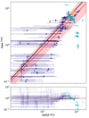 |
Fig. 6. Correlation between observed frequency νQPO and the Kepler frequency at the transition radius νK(rJ) (top), as well as the residuals defined as the ratio between the best weighted fit (in red) and the data (bottom). In their own colors, different types of quasi-periodic oscillations: Type A in light-yellow, Type B in cyan, Type C in dark-blue. In red the weighed linear fit considering only Type C LFQPOs, νQPO = (10 ± 3) × 10−3 ⋅ νK(rJ)0.96 ± 0.04, in black the νQPO = νK(rJ)/100 line. |
This correlation is drawn in red on Fig. 6. This is an excellent correlation considering the important error-bars implied and the simplicity of the fitting procedure. Notably, the index 0.96 ± 0.04 (1σ error), close to 1, suggests that νQPO ∝ νK(rJ). When forcing a slope of 1, the best weighted fit results in νQPO ≃ (7.5 ± 0.2) × 10−3 ⋅ νK(rJ), i.e. a factor q = 133 ± 4 between νQPO and νK(rJ).
This is the first time that such a correlation is displayed for GX 339-4, but multiple studies found very similar results for other X-ray binaries: GRS 1915+105 (Muno et al. 1999; Trudolyubov et al. 1999; Rodriguez et al. 2002), XTE J1748-288 (Revnivtsev et al. 2000), XTE J1550-564 (Sobczak et al. 2000; Rodriguez et al. 2004), and GRO J1655-40 (Sobczak et al. 2000). In these studies, a correlation between the frequency of the Type C QPOs and the inner radius of an optically thick disk (i.e., similar to rJ here at low luminosities), and displayed correlations νQPO ∼ νK(rJ)/q, with q in the range 50 − 150. In our study, we found q = 133 ± 4, and varying between outbursts: q#1 = 133 ± 5, q#2 = 97 ± 5, q#3 = 136 ± 5, and q#4 = 75 ± 11, see from Figs. B.1 to B.4. A variation in q between outbursts and/or objects would be a major constraint for QPO models, but unfortunately the lack of statistics and the important error-bars prevent us from drawing any conclusion with the present study.
Additionally, although we only fitted using Type C LFQPOs, the best fit also seems to capture Type A. However, Type B quasi-periodic oscillations do not follow the same correlation. Type B have a much lower frequency than the correlation in Fig. 6, by a factor of up to ∼10. The factor q ∼ 100 between νQPO and νK(rJ) needs now to be as high as ∼1000. It is hard to imagine a process, even secular, to resolve this discrepancy. For this reason, it would be natural to consider that Type B are produced via a process different from Type A and Type C. However, Type B are detected at tiny transition radii (i.e., high Kepler frequencies), when relativistic effects are important. Rather than the usual Kepler frequency, we examine below if using the epicyclic frequency at the transition radius could solve this issue (see Varnière et al. 2002).
3.4. Correlation with transition radius
We display the correlation between νQPO and rJ in Fig. 7. Due to general relativistic effects, one should consider in this section the epicyclic frequency (Varnière et al. 2002),
 (3)
(3)
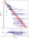 |
Fig. 7. Correlation between observed frequency νQPO and the transition radius rJ (top), as well as the residuals defined as the ratio between the best weighted fit (in red) and the data (bottom). In their own colors, different types of quasi-periodic oscillations: Type A in light-yellow, Type B in cyan, Type C in dark-blue. In red the weighed linear fit considering only Type C LFQPOs, |
where we retrieve νep = νK(rJ) for rJ ≫ risco. Because these two frequencies are similar until rJ ≳ risco, νK(rJ) and νep(rJ) follow a similar correlation with frequencies 2 orders of magnitude too high νQPO = νep(rJ)/100. Both these correlations are shown on Fig. 7: in black νQPO = νK(rJ)/100, in dashed-black νQPO = νep(rJ)/100. Again, the black curve meets well with the best fit (in red).
Considering this new νQPO = νep(rJ)/100 slope, what resembles a shift by a factor 10 in νQPO in Fig. 6 can in fact be interpreted as a shift by a factor ∼1.5 in rJ in Fig. 7. If rJ was smaller than calculated by our model, say rJ = 2.1 − 2.5 instead of rJ ∼ 3 − 4, then these Type B QPOs (cyan) could in principle fit in the dashed-black correlation10. An overestimate of rJ for Type B QPOs can have two major causes. First, our model does not include all possible effects; a different transition radius could be obtained if one includes a relativistic treatment of the equations, ray-tracing effects, or gravitational red-shifts for example. Second, as discussed previously in Sect. 2.3, the difference between soft-intermediate (rJ ∼ 3 − 4) and soft-states (rJ = risco = 2) is not clear-cut in our fits. A better treatment of the hard tail could very well lead to over/under-estimates of the transition radius once such small values are reached. However, we note that Type C QPOs are well behaved for even the smallest transition radii (rJ < 3), while Type B QPOs have already diverged from the correlation at rJ = 4 − 5. This difference suggests that small transition radii are not primarily responsible for pushing Type B QPOs off the correlation above. Although it is tempting to try to correct the transition radius, we believe this is premature given the points above. Instead, these features likely follow a different correlation entirely, as some previous studies have suggested already (see e.g., Motta et al. 2011). We would like to point out that the transition from some Type C to Type B appears smooth in the two residuals at the bottom of Figs. 6 and 7, suggesting further relationships between Type B and Type C QPOs that will be explored in a future work.
4. Summary and conclusions
In this paper, we assume that the accretion flow is separated in two different regions, an inner jet-emitting disk and an outer standard accretion disk: The JED-SAD paradigm (Paper I). We use tools and methods detailed in the previous papers of this series (Papers II–IV) to address some timing properties of the hybrid JED-SAD configuration for the first time. We summarize the methods and the major results from this study in three points:
First, we select RXTE/PCA (X-ray) and ATCA (radio) data covering three outbursts of GX 339-4. We then use the procedure detailed in Paper IV for a previous outburst to obtain an estimate of (rJ,ṁin) in the JED-SAD paradigm during these three new outbursts. The dynamical insights from the study of the four outbursts will be discussed in a forthcoming paper, but it is already important to note that a unique multiplication factor  was used to estimate the radio flux. In other words, the jet radiative efficiency is constant during all four outbursts, although the jets are quenched during each soft state.
Second, we use the same RXTE/PCA data and focus on a study of LFQPOs. We report the detection of 7 new LFQPOs (see Table C.2).
Third and more importantly, we confirm that the frequency of Type C QPOs can be linked to the transition radius between two different accretion flows (JED and SAD here). This correlation requires a (surprising) factor q between the Kepler frequencies at the transition radius and the QPO frequencies, varying between ∼70 and ∼130 for different outbursts, with a value q = 133 ± 4 for all four outbursts combined. Such a factor is hard to estimate, but multiple studies have shown to require two orders of magnitude between the QPO and Kepler frequencies around different objects (see Sect. 3). However, while these former studies envisioned that QPOs were linked to the optically thick-to-thin transition in the flow, we argue and show here a link between QPOs and the transition radius between the inner magnetized (μ ∼ 0.5) and an outer weakly magnetized (μ ≪ 1) flow. This link indicates that QPOs must be created by a secular (given the high value of q) instability/process related to the dynamical JED-SAD transition and thus, somehow, connected to the jets. This connection is consistent with previous suggestions of a link between the existence of jets and the presence of QPOs (Fender et al. 2009), but this is, to our knowledge, the first time that the direct link is displayed (see Sect. 4.3 in Uttley & Casella 2014). Moreover, such connection is supported by the observed relations between IR and X-ray QPOs (Casella et al. 2010; Kalamkar et al. 2016; Vincentelli et al. 2019), a behavior that current models fail to address.
Because of the remarkable correlation between Type C QPOs and rJ, these results provide an independent support to the JED-SAD paradigm. However, the apparent differences between QPO types need to be addressed, and the processe(s) to produce the LFQPOs in this paradigm remain to be discussed.
We would like to point out that in some cases the system never reaches the soft state before the luminosity decreases back to quiescence: such outbursts are referred to as failed, or hard-only, outbursts (Tetarenko et al. 2016).
See also for example Thorne & Price (1975), Shapiro et al. (1976), Oda (1977), Abramowicz et al. (1980), or Lasota et al. (1996).
The fluxes were extrapolated over the 3 − 200 keV range, see Sect. 3.1 in Paper IV.
In the previous papers of this series, we used a notation rin for risco. We however decided to use only risco now to avoid any ambiguity with the inner radius of other models, often labeled rint.
The figure for outburst #4 is reported here for comparison, but is the same as Fig. 7 in Paper IV.
For other differences in the continuum, rms, QPO types, or broad band noise, see Marcel et al. (in prep.).
Equivalently, one can link the QPO frequency to a given radius rQPO. Such a radius would thus be a factor ∼1002/3 ∼ 20 bigger than our typical transition radius rJ.
We recall here that the spectral states were defined solely on the X-ray continuum (disk and power-law), independently from the presence of any (type of) QPO.
While we argued earlier that the self-similar assumption might not hold for the smallest values of rJ, this argument is irrelevant regarding QPOs: The possibility to have QPOs even for rJ ≳ risco depends on the processus involved in their production.
Acknowledgments
We thank the anonymous referee for helpful comments and careful reading of the manuscript. The authors acknowledge funding support from the french research national agency (CHAOS project ANR-12-BS05-0009, https://ipag.osug.fr/ANR-CHAOS/), centre national d’études spatiales (CNES), and the programme national des hautes énergies (PNHE). This research has made use of data, software, and/or web tools obtained from the high energy astrophysics science archive research center (HEASARC), a service of the astrophysics science division at NASA/GSFC. Figures in this paper were produced using the MATPLOTLIB package (Hunter 2007), and weighted fits using the SciPy package (Virtanen et al. 2020).
References
- Abramowicz, M. A., Calvani, M., & Nobili, L. 1980, ApJ, 242, 772 [NASA ADS] [CrossRef] [Google Scholar]
- Beloborodov, A. M. 1999, ASP Conf. Ser., 161, 295 [Google Scholar]
- Blandford, R. D., & Königl, A. 1979, ApJ, 232, 34 [NASA ADS] [CrossRef] [Google Scholar]
- Blandford, R. D., & Payne, D. G. 1982, MNRAS, 199, 883 [NASA ADS] [CrossRef] [Google Scholar]
- Casella, P., Belloni, T., & Stella, L. 2005, ApJ, 629, 403 [NASA ADS] [CrossRef] [Google Scholar]
- Casella, P., Maccarone, T. J., O’Brien, K., et al. 2010, MNRAS, 404, L21 [NASA ADS] [Google Scholar]
- Clavel, M., Rodriguez, J., Corbel, S., & Coriat, M. 2016, Astron. Nachr., 337, 435 [NASA ADS] [CrossRef] [Google Scholar]
- Corbel, S., Fender, R. P., Tomsick, J. A., Tzioumis, A. K., & Tingay, S. 2004, ApJ, 617, 1272 [NASA ADS] [CrossRef] [Google Scholar]
- Corbel, S., Aussel, H., Broderick, J. W., et al. 2013a, MNRAS, 431, L107 [NASA ADS] [CrossRef] [Google Scholar]
- Corbel, S., Coriat, M., Brocksopp, C., et al. 2013b, MNRAS, 428, 2500 [NASA ADS] [CrossRef] [Google Scholar]
- Done, C., Gierliński, M., & Kubota, A. 2007, A&ARv, 15, 1 [NASA ADS] [CrossRef] [EDP Sciences] [Google Scholar]
- Drappeau, S., Malzac, J., Coriat, M., et al. 2017, MNRAS, 466, 4272 [NASA ADS] [Google Scholar]
- Dunn, R. J. H., Fender, R. P., Körding, E. G., Belloni, T., & Cabanac, C. 2010, MNRAS, 403, 61 [NASA ADS] [CrossRef] [Google Scholar]
- Eddington, A. S. 1926, The Internal Constitution of the Stars (Cambridge: Cambridge University Press) [Google Scholar]
- Esin, A. A., McClintock, J. E., & Narayan, R. 1997, ApJ, 489, 865 [NASA ADS] [CrossRef] [Google Scholar]
- Fender, R. P., Belloni, T. M., & Gallo, E. 2004, MNRAS, 355, 1105 [NASA ADS] [CrossRef] [Google Scholar]
- Fender, R. P., Homan, J., & Belloni, T. M. 2009, MNRAS, 396, 1370 [NASA ADS] [CrossRef] [Google Scholar]
- Ferreira, J. 1997, A&A, 319, 340 [Google Scholar]
- Ferreira, J., Petrucci, P. O., Henri, G., Saugé, L., & Pelletier, G. 2006, A&A, 447, 813 [NASA ADS] [CrossRef] [EDP Sciences] [Google Scholar]
- Gao, H. Q., Qu, J. L., Zhang, Z., et al. 2014, MNRAS, 438, 341 [CrossRef] [Google Scholar]
- García, J. A., Steiner, J. F., McClintock, J. E., et al. 2015, ApJ, 813, 84 [NASA ADS] [CrossRef] [Google Scholar]
- Heida, M., Jonker, P. G., Torres, M. A. P., & Chiavassa, A. 2017, ApJ, 846, 132 [NASA ADS] [CrossRef] [Google Scholar]
- Heinz, S., & Sunyaev, R. A. 2003, MNRAS, 343, L59 [NASA ADS] [CrossRef] [Google Scholar]
- Homan, J., Miller, J. M., Wijnands, R., et al. 2005, ApJ, 623, 383 [NASA ADS] [CrossRef] [Google Scholar]
- Hunter, J. D. 2007, Comput. Sci. Eng., 9, 90 [NASA ADS] [CrossRef] [Google Scholar]
- Hynes, R. I., Steeghs, D., Casares, J., Charles, P. A., & O’Brien, K. 2003, ApJ, 583, L95 [NASA ADS] [CrossRef] [Google Scholar]
- Hynes, R. I., Steeghs, D., Casares, J., Charles, P. A., & O’Brien, K. 2004, ApJ, 609, 317 [NASA ADS] [CrossRef] [Google Scholar]
- Ichimaru, S. 1977, ApJ, 214, 840 [NASA ADS] [CrossRef] [Google Scholar]
- Ingram, A., & Motta, S. 2020, New Astron. Rev., submitted [arXiv:2001.08758] [Google Scholar]
- Kalamkar, M., Casella, P., Uttley, P., et al. 2016, MNRAS, 460, 3284 [NASA ADS] [CrossRef] [Google Scholar]
- Körding, E. G., Jester, S., & Fender, R. 2006, MNRAS, 372, 1366 [NASA ADS] [CrossRef] [Google Scholar]
- Lasota, J. P., Narayan, R., & Yi, I. 1996, A&A, 314, 813 [NASA ADS] [Google Scholar]
- Liska, M., Tchekhovskoy, A., Ingram, A., & van der Klis, M. 2019, MNRAS, 487, 550 [NASA ADS] [CrossRef] [Google Scholar]
- Marcel, G., Ferreira, J., Petrucci, P. O., et al. 2018a, A&A, 617, A46 [NASA ADS] [CrossRef] [EDP Sciences] [Google Scholar]
- Marcel, G., Ferreira, J., Petrucci, P. O., et al. 2018b, A&A, 615, A57 [NASA ADS] [CrossRef] [EDP Sciences] [Google Scholar]
- Marcel, G., Ferreira, J., Clavel, M., et al. 2019, A&A, 626, A115 [NASA ADS] [CrossRef] [EDP Sciences] [Google Scholar]
- McClintock, J. E., & Remillard, R. A. 2006, Black Hole Binaries, 39, 157 [Google Scholar]
- Miller, J. M., Reynolds, C. S., Fabian, A. C., et al. 2008, ApJ, 679, L113 [NASA ADS] [CrossRef] [Google Scholar]
- Mirabel, I. F., Rodriguez, L. F., Cordier, B., Paul, J., & Lebrun, F. 1992, Nature, 358, 215 [NASA ADS] [CrossRef] [Google Scholar]
- Miyamoto, S., & Matsuoka, M. 1977, Space Sci. Rev., 20, 687 [NASA ADS] [CrossRef] [Google Scholar]
- Miyamoto, S., Kimura, K., Kitamoto, S., Dotani, T., & Ebisawa, K. 1991, ApJ, 383, 784 [NASA ADS] [CrossRef] [Google Scholar]
- Motta, S. E. 2016, Astron. Nachr., 337, 398 [NASA ADS] [CrossRef] [Google Scholar]
- Motta, S., Muñoz-Darias, T., Casella, P., Belloni, T., & Homan, J. 2011, MNRAS, 418, 2292 [NASA ADS] [CrossRef] [Google Scholar]
- Muñoz-Darias, T., Casares, J., & Martínez-Pais, I. G. 2008, MNRAS, 385, 2205 [NASA ADS] [CrossRef] [Google Scholar]
- Muno, M. P., Morgan, E. H., & Remillard, R. A. 1999, ApJ, 527, 321 [NASA ADS] [CrossRef] [Google Scholar]
- Nandi, A., Debnath, D., Mandal, S., & Chakrabarti, S. K. 2012, A&A, 542, A56 [NASA ADS] [CrossRef] [EDP Sciences] [Google Scholar]
- Narayan, R., & Yi, I. 1994, ApJ, 428, L13 [NASA ADS] [CrossRef] [Google Scholar]
- Oda, M. 1977, Space Sci. Rev., 20, 757 [CrossRef] [Google Scholar]
- Parker, M. L., Tomsick, J. A., Kennea, J. A., et al. 2016, ApJ, 821, L6 [NASA ADS] [CrossRef] [Google Scholar]
- Rees, M. J., Begelman, M. C., Blandford, R. D., & Phinney, E. S. 1982, Nature, 295, 17 [NASA ADS] [CrossRef] [Google Scholar]
- Reis, R. C., Fabian, A. C., Ross, R. R., et al. 2008, MNRAS, 387, 1489 [NASA ADS] [CrossRef] [Google Scholar]
- Remillard, R. A., & McClintock, J. E. 2006, ARA&A, 44, 49 [NASA ADS] [CrossRef] [Google Scholar]
- Revnivtsev, M. G., Trudolyubov, S. P., & Borozdin, K. N. 2000, MNRAS, 312, 151 [NASA ADS] [CrossRef] [Google Scholar]
- Rodriguez, J., Varnière, P., Tagger, M., & Durouchoux, P. 2002, A&A, 387, 487 [NASA ADS] [CrossRef] [EDP Sciences] [Google Scholar]
- Rodriguez, J., Corbel, S., Kalemci, E., Tomsick, J. A., & Tagger, M. 2004, ApJ, 612, 1018 [NASA ADS] [CrossRef] [Google Scholar]
- Samimi, J., Share, G. H., Wood, K., et al. 1979, Nature, 278, 434 [NASA ADS] [CrossRef] [Google Scholar]
- Scepi, N., Dubus, G., & Lesur, G. 2019, A&A, 626, A116 [NASA ADS] [CrossRef] [EDP Sciences] [Google Scholar]
- Shakura, N. I., & Sunyaev, R. A. 1973, A&A, 24, 337 [NASA ADS] [Google Scholar]
- Shapiro, S. L., Lightman, A. P., & Eardley, D. M. 1976, ApJ, 204, 187 [NASA ADS] [CrossRef] [Google Scholar]
- Sobczak, G. J., McClintock, J. E., Remillard, R. A., et al. 2000, ApJ, 531, 537 [NASA ADS] [CrossRef] [Google Scholar]
- Tetarenko, B. E., Sivakoff, G. R., Heinke, C. O., & Gladstone, J. C. 2016, ApJS, 222, 15 [NASA ADS] [CrossRef] [Google Scholar]
- Thorne, K. S., & Price, R. H. 1975, ApJ, 195, L101 [NASA ADS] [CrossRef] [Google Scholar]
- Trudolyubov, S. P., Churazov, E. M., & Gilfanov, M. R. 1999, Astron. Lett., 25, 718 [Google Scholar]
- Uttley, P., & Casella, P. 2014, Space Sci. Rev., 183, 453 [NASA ADS] [CrossRef] [Google Scholar]
- van der Klis, M. 1989, ARA&A, 27, 517 [NASA ADS] [CrossRef] [Google Scholar]
- Varnière, P., & Rodriguez, J. 2018, ApJ, 865, 113 [NASA ADS] [CrossRef] [Google Scholar]
- Varnière, P., Rodriguez, J., & Tagger, M. 2002, A&A, 387, 497 [NASA ADS] [CrossRef] [EDP Sciences] [Google Scholar]
- Vincentelli, F. M., Casella, P., Petrucci, P., et al. 2019, ApJ, 887, L19 [CrossRef] [Google Scholar]
- Virtanen, P., Gommers, R., Oliphant, T. E., et al. 2020, Nat. Methods, 17, 261 [Google Scholar]
- Yuan, F., & Narayan, R. 2014, ARA&A, 52, 529 [NASA ADS] [CrossRef] [Google Scholar]
- Zdziarski, A. A., Poutanen, J., Mikolajewska, J., et al. 1998, MNRAS, 301, 435 [NASA ADS] [CrossRef] [Google Scholar]
- Zdziarski, A. A., Gierliński, M., Mikołajewska, J., et al. 2004, MNRAS, 351, 791 [NASA ADS] [CrossRef] [Google Scholar]
- Zhang, S.-N. 2013, Front. Phys., 8, 630 [NASA ADS] [CrossRef] [Google Scholar]
- Zhang, L., Wang, Y., Méndez, M., et al. 2017, ApJ, 845, 143 [CrossRef] [Google Scholar]
Appendix A: Discrepancies on QPO identifications
In this section, we provide the fitting results of the PDS to illustrate the differences with previous studies.
In obsID 70110-01-10-00, Motta et al. (2011) reported a  Hz Type C QPO. However, when performing the fit, we believe that this component is in fact an harmonic for 2 major reasons (see Fig. A.1). First, there is a very strong component at
  Hz with very high coherence factor Q = 8.16. Second, there is another harmonic component at
  Hz, consistent with being 3 times the frequency of the
  Hz QPO. We thus have the fundamental at ν0 = 2.06 Hz, and two harmonic component at ν1 = 4.20 Hz ≃ 2ν0 and ν2 = 6.67 Hz ≃ 3ν0.
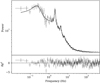 |
Fig. A.1. Power spectrum of obsID 70110-01-10-00. |
In obsID 92085-01-03-00, two major components are present at 3.96 Hz and 7.72 Hz (see Fig. A.2). While the components have similar coherence factors Q = 2.87 for the 7.72 Hz QPO and Q = 2.52 for the 3.96 Hz QPO, the time evolution is key here. Both QPOs before and after obsID 92085-01-03-00 have frequencies closer to 7.72 Hz (see Table C.1), suggesting that the QPO we are following in this rising outburst is at 7.72 Hz: we agree with Motta et al. (2011) about the fundamental component. However, they reported this QPO as a Type C, and we strongly believe it should be classified as a Type B for two reasons. First, the previous and following QPOs were Type B (ignoring Type A, see Table C.1). Second, the power spectrum does not show any broad band noise, a key characteristic of Type C QPOs. We thus decide to keep the QPO of highest frequency, but we classify it as a Type B, unlike Motta et al. (2011).
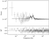 |
Fig. A.2. Power spectrum of obsID 92085-01-03-00. |
Similarly, in obsID 92085-01-03-03, Motta et al. (2011) report the detection of a Type C QPO at 7.00 Hz. However, the power spectrum does not show significant broad band noise (see Fig. A.3). This could very well be a result of the different procedure used, or a matter of definition, but to be fully consistent within our study we decided to keep that QPO as a Type B.
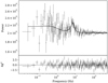 |
Fig. A.3. Power spectrum of obsID 92085-01-03-03. |
Finally in obsID 95409-01-17-02, Motta et al. (2011) report a 6.67 Hz Type C QPO, while Nandi et al. (2012) report a 6.65 Hz Type B QPO. While the time evolution seems to suggest that this QPO is a Type B (see Table C.1), we identify this to be a 6.66 Hz Type C QPO, due to the presence of a significant broad band noise in the power spectrum (see Fig. A.4).
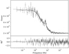 |
Fig. A.4. Power spectrum of obsID 95409-01-17-02. |
Appendix B: Correlation with Kepler frequency for each outburst
In this section, we show the correlation of the QPO frequency νQPO as function of the Kepler frequency at the transition radius νK(rJ) for all 4 different outbursts.
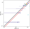 |
Fig. B.1. Correlation between observed frequency νQPO and the Kepler frequency at the transition radius νK(rJ) for outburst #1. In their own colors, different types of quasi-periodic oscillations: Type A in light-yellow, Type B in cyan, Type C in dark-blue. In red the weighed linear best fit with slope 1 considering only Type C LFQPOs, νQPO = (7.5 ± 0.3) × 10−3 ⋅ νK(rJ), in black the νQPO = νK(rJ)/100 line. |
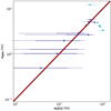 |
Fig. B.2. Correlation between observed frequency νQPO and the Kepler frequency at the transition radius νK(rJ) for outburst #2. This figure is similar to Fig. B.1, but this time νQPO = (10.4 ± 0.5) × 10−3 ⋅ νK(rJ). |
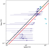 |
Fig. B.3. Correlation between observed frequency νQPO and the Kepler frequency at the transition radius νK(rJ) for outburst #3. This figure is similar to Fig. B.1, but this time νQPO = (7.4 ± 0.3) × 10−3 ⋅ νK(rJ). |
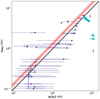 |
Fig. B.4. Correlation between observed frequency νQPO and the Kepler frequency at the transition radius νK(rJ) for outburst #4. This figure is similar to Fig. B.1, but this time νQPO = (13.4 ± 0.2) × 10−3 ⋅ νK(rJ). |
Appendix C: Detected LFQPOs
We report in the following tables the quasi-periodic oscillations detected in this study. See Sect. 2.1 for the data involved and Sect. 2.4.1 for the method used. In the first table we show all the fundamentals detected QPOs in the literature and in this study, in the second table we show only the new ones from this study.
All detected QPOs from this work and previous studies.
Newly detected QPOs in RXTE/PCA data from GX 339-4.
All Tables
Four full cycles from GX 339-4 during the 2001–2011 decade and their associated number of observations in X-rays and radio.
Number of reported (fundamental) LFQPOs in GX 339-4 using the RXTE/PCA observations.
All Figures
|
Fig. 1. RTXE/PCA lightcurves of GX 339-4 in the 3 − 200 keV energy band from 2002 to 2011 (see upper X-axis). In filled colors, the power-law (violet), and disk (cyan) unabsorbed fluxes from the Clavel et al. (2016) fits. In gray, the area corresponding to the 4 complete outbursts (#1, #2, #3, #4). Red lines at the top correspond to dates when steady radio fluxes were observed with the Australia telescope compact array (ATCA) at 9 GHz (Corbel et al. 2013a,b). Yellow lines at the bottom show previous detections of quasi-periodic oscillations (QPO, Motta et al. 2011; Nandi et al. 2012; Gao et al. 2014; Zhang et al. 2017). |
| In the text | |
|
Fig. 2. Observation and model parameters for cycles #1 (2002–2003, left) and #2 (2004–2005, right). From top to bottom: X-ray flux and power-law fraction in the 3 − 200 keV range, power-law index, 9 GHz radio flux, transition radius rJ, and inner accretion rate ṁin (at ISCO). For the first 4 panels, i.e., the constraints, black squares are observations. Each figure uses the same color-code: green upper- (lower-) triangles for the rising (decaying) hard, blue circles for hard-intermediate, yellow crosses for soft-intermediate, and red crosses for soft-states. Additionally, in the state-associated colors we draw the 5% and 10% confidence intervals (i.e., 5% and 10% bigger ζX + R, see Paper IV). Double arrows are drawn when radio emission was also observed but has been interpreted as radio flares or interactions with the interstellar medium (Corbel et al., in prep.). |
| In the text | |
|
Fig. 3. Observation and model parameters for cycles #3 (2006–2007, left) and #4 (2010–2011, right). From top to bottom: X-ray flux and power-law fraction in the 3 − 200 keV range, power-law index, 9 GHz radio flux, transition radius rJ, and inner accretion rate ṁin (at ISCO). For the first 4 panels, i.e., the constraints, black squares are observations. Each figure uses the same color-code: green upper- (lower-) triangles for the rising (decaying) hard, blue circles for hard-intermediate, yellow crosses for soft-intermediate, and red crosses for soft-states. Additionally, in the state-associated colors we draw the 5% and 10% confidence intervals (i.e., 5% and 10% bigger ζX + R, see Paper IV). Double arrows are drawn when radio emission was also observed but has been interpreted as radio flares or interactions with the interstellar medium (Corbel et al., in prep.). |
| In the text | |
|
Fig. 4. DFLDs showing the distribution of states (top) and observed LFQPOs (bottom). Top panel: states are shown in the same color-code as in Figs. 2 and 3 (see legend). Bottom panel: in different colors, position where QPOs were identified (see legend). Light gray squares in background are observations from Clavel et al. (2016). |
| In the text | |
|
Fig. 5. Co-evolution of the observed QPO frequency νQPO and the Kepler rotation frequency νK(rJ) for the 4 different outbursts, showing both hard-to-soft and soft-to-hard transitions (see red annotations). On the left Y-axis, the Kepler frequency at the transition radius, νK(rJ), and the 5% and 10% confidence intervals. On the right Y-axis, the observed QPO frequency, νQPO. Different markers are used to disentangle the different works: Motta et al. (2011) in upper-triangles, Nandi et al. (2012) in lower-triangles, Gao et al. (2014) in crosses, Zhang et al. (2017) in plus signs, and new detections in circle markers (see text). We also use different colors for the different types of QPOs (see legend). |
| In the text | |
|
Fig. 6. Correlation between observed frequency νQPO and the Kepler frequency at the transition radius νK(rJ) (top), as well as the residuals defined as the ratio between the best weighted fit (in red) and the data (bottom). In their own colors, different types of quasi-periodic oscillations: Type A in light-yellow, Type B in cyan, Type C in dark-blue. In red the weighed linear fit considering only Type C LFQPOs, νQPO = (10 ± 3) × 10−3 ⋅ νK(rJ)0.96 ± 0.04, in black the νQPO = νK(rJ)/100 line. |
| In the text | |
|
Fig. 7. Correlation between observed frequency νQPO and the transition radius rJ (top), as well as the residuals defined as the ratio between the best weighted fit (in red) and the data (bottom). In their own colors, different types of quasi-periodic oscillations: Type A in light-yellow, Type B in cyan, Type C in dark-blue. In red the weighed linear fit considering only Type C LFQPOs, |
| In the text | |
|
Fig. A.1. Power spectrum of obsID 70110-01-10-00. |
| In the text | |
|
Fig. A.2. Power spectrum of obsID 92085-01-03-00. |
| In the text | |
|
Fig. A.3. Power spectrum of obsID 92085-01-03-03. |
| In the text | |
|
Fig. A.4. Power spectrum of obsID 95409-01-17-02. |
| In the text | |
|
Fig. B.1. Correlation between observed frequency νQPO and the Kepler frequency at the transition radius νK(rJ) for outburst #1. In their own colors, different types of quasi-periodic oscillations: Type A in light-yellow, Type B in cyan, Type C in dark-blue. In red the weighed linear best fit with slope 1 considering only Type C LFQPOs, νQPO = (7.5 ± 0.3) × 10−3 ⋅ νK(rJ), in black the νQPO = νK(rJ)/100 line. |
| In the text | |
|
Fig. B.2. Correlation between observed frequency νQPO and the Kepler frequency at the transition radius νK(rJ) for outburst #2. This figure is similar to Fig. B.1, but this time νQPO = (10.4 ± 0.5) × 10−3 ⋅ νK(rJ). |
| In the text | |
|
Fig. B.3. Correlation between observed frequency νQPO and the Kepler frequency at the transition radius νK(rJ) for outburst #3. This figure is similar to Fig. B.1, but this time νQPO = (7.4 ± 0.3) × 10−3 ⋅ νK(rJ). |
| In the text | |
|
Fig. B.4. Correlation between observed frequency νQPO and the Kepler frequency at the transition radius νK(rJ) for outburst #4. This figure is similar to Fig. B.1, but this time νQPO = (13.4 ± 0.2) × 10−3 ⋅ νK(rJ). |
| In the text | |
Current usage metrics show cumulative count of Article Views (full-text article views including HTML views, PDF and ePub downloads, according to the available data) and Abstracts Views on Vision4Press platform.
Data correspond to usage on the plateform after 2015. The current usage metrics is available 48-96 hours after online publication and is updated daily on week days.
Initial download of the metrics may take a while.