| Issue |
A&A
Volume 639, July 2020
|
|
|---|---|---|
| Article Number | A114 | |
| Number of page(s) | 8 | |
| Section | The Sun and the Heliosphere | |
| DOI | https://doi.org/10.1051/0004-6361/202038433 | |
| Published online | 21 July 2020 | |
Ultra-long and quite thin coronal loop without significant expansion⋆
1
Key Laboratory of Dark Matter and Space Astronomy, Purple Mountain Observatory, CAS, Nanjing 210033, PR China
e-mail: lidong@pmo.ac.cn
2
State Key Laboratory of Space Weather, Chinese Academy of Sciences, Beijing 100190, PR China
3
Institute of Space Science and Applied Technology, Harbin Institute of Technology, Shenzhen 518055, PR China
e-mail: yuanding@hit.edu.cn
4
Centre for Mathematical Plasma Astrophysics, Department of Mathematics, KU Leuven, Celestijnenlaan 200B, 3001 Leuven, Belgium
5
MOE Key Laboratory of Fundamental Physical Quantities Measurements, School of Physics, Huazhong University of Science and Technology, Wuhan 430074, PR China
6
School of Astronomy and Space Science, University of Science and Technology of China, Hefei 230026, PR China
Received:
18
May
2020
Accepted:
3
June
2020
Context. Coronal loops are the basic building blocks of the solar corona. They are related to the mass supply and heating of solar plasmas in the corona. However, their fundamental magnetic structures are still not well understood. Most coronal loops do not expand significantly, but the diverging magnetic field would have an expansion factor of about 5−10 over one pressure scale height.
Aims. We investigate a unique coronal loop with a roughly constant cross section. The loop is ultra long and quite thin. A coronal loop model with magnetic helicity is presented to explain the small expansion of the loop width.
Methods. This coronal loop was predominantly detectable in the 171 Å channel of the Atmospheric Imaging Assembly (AIA). Then, the local magnetic field line was extrapolated within a model of the potential field source-surface. Finally, the differential emission measure analysis made from six AIA bandpasses was applied to obtain the thermal properties of this loop.
Results. This coronal loop has a projected length of roughly 130 Mm, a width of about 1.5 ± 0.5 Mm, and a lifetime of about 90 min. It follows an open magnetic field line. The cross section expanded very little (i.e., 1.5−2.0) along the loop length during its whole lifetime. This loop has a nearly constant temperature at about 0.7 ± 0.2 MK, but its density exhibits the typical structure of a stratified atmosphere.
Conclusions. We use the theory of a thin twisted flux tube to construct a model for this nonexpanding loop and find that with sufficient twist, a coronal loop can indeed attain equilibrium. However, we cannot rule out other possibilities such as footpoint heating by small-scale reconnection or an elevated scale height by a steady flow along the loop.
Key words: Sun: corona / Sun: UV radiation / Sun: magnetic fields / Sun: activity
Movie is available at https://www.aanda.org
© ESO 2020
1. Introduction
Coronal loops are the basic structures in the solar corona. They can be detected everywhere on the Sun, such as in quiet regions, active regions, or on the solar limb, and their size can range from sub-megameters to hundreds of megameters in the lower corona. These coronal loops often confine plasma at a temperature of mega-Kelvin, therefore they are prominently detectable in the extreme-ultraviolet (EUV) and X-ray bandpasses (Bray et al. 1991; Reale 2014). Moreover, the plasmas contained in a coronal loop may be either isothermal (e.g., Del Zanna & Mason 2003; Tripathi et al. 2009; Gupta et al. 2019) or multithermal (e.g., Schmelz & Martens 2006; Kucera et al. 2019) along the line of sight. In the corona, fully ionized plasma is frozen-in in the magnetic field line. This means that the plasma properties are normally uniform along the loops, and strong inhomogeneity is usually detected across the loops. By comparisons of the coronal imaging observations in EUV or X-ray channels, together with the extrapolated field lines derived from the photospheric magnetogram, the coronal loop was found to generally follow the magnetic field line (Poletto et al. 1975; Feng et al. 2007). That is, a closed coronal loop usually consists of a loop apex and two footpoints that are rooted in two opposite polarities (e.g., Watko & Klimchuk 2000; Peter & Bingert 2012), while an open coronal loop connects to one apparent polarity at the solar surface and extends radially into the heliosphere magnetic field (e.g., Gupta et al. 2019). Previous studies also suggested that the temperature variation along a coronal loop is highly sensitive to the heating mechanism (Priest et al. 1998; Warren et al. 2008). Therefore studying the coronal loop in the complex magnetic environment can help us understand the fundamental problem in solar physics better. This fundamental problm is coronal heating (e.g., Klimchuk 2000; Peter & Bingert 2012; Li et al. 2015; Goddard et al. 2017).
The coronal loop is expected to expand with height because the coronal magnetic field is found to diverge strongly with height from the solar surface into the corona (Lionello et al. 2013; Chen et al. 2014). The expansion of a coronal loop was discovered in an active region (e.g., Malanushenko & Schrijver 2013) or on a solar limb (e.g., Gupta et al. 2019). However, most coronal loops observed in X-ray and EUV images are found to have roughly uniform widths in the plane of the sky, without significant expansions along their loop lengths, or they only exhibit a small expansion from footpoints to the loop apex (e.g., Golub et al. 1990; Klimchuk et al. 1992; Klimchuk 2000; Watko & Klimchuk 2000; López Fuentes et al. 2006; Brooks et al. 2007; Kucera et al. 2019). The formation and appearance of these loops in the complex magnetic environment of the corona provides a pivotal test for a model of the coronal heating process (Klimchuk 2000; Petrie 2006; Peter & Bingert 2012). On the other hand, the loop cross section carries information of magnetic fields and the spatial distribution of corona heating, and the lower limit of the loop width is of fundamental importance to modern instrumentation because it defines the spatial resolution of a space-borne or ground-based telescope (Peter et al. 2013; Aschwanden & Peter 2017). Moreover, the loop width variation is a proxy of the inter-coupling of plasma dynamics and magnetic fields, therefore it is believed to play a key role in coronal heating (e.g., Vesecky et al. 1979; McTiernan & Petrosian 1990; Mikić et al. 2013; Chastain & Schmelz 2017). Aschwanden & Peter (2017) found that the loop widths are only marginally resolved in AIA images, but are fully resolved in Hi-C images. Their model predicts a most frequent value at about 0.55 Mm.
The contradiction between the observed coronal loop with a roughly constant cross section and the extrapolated magnetic field with a strong expansion is still not explained. In this paper, we investigate an ultra-long but quite thin coronal loop that might be explained by a thin twisted flux tube model. The paper is organized as follows: Sect. 2 introduces the data reduction and methods, Sect. 3 describes the properties of the coronal loop of interest, and the conclusion and discussion are presented in Sect. 4.
2. Data reduction and methods
2.1. Data reduction
We combined data obtained with the Atmospheric Imaging Assembly (AIA; Lemen et al. 2012) and the Helioseismic Magnetic Imager (HMI; Schou et al. 2012) on board the Solar Dynamic Observatory (SDO; Pesnell et al. 2012) to observe active region NOAA 12524 near solar disk center (N20W04) on 2016 March 23. A unique coronal loop was predominately observed in the AIA 171 Å channel. It was also vaguely simultaneously detectable in the AIA 193 Å and 211 Å channels, as shown in Figs. 1a−c. This loop was ultra long and very narrow, and it did not expand much radially along its length. Moreover, this coronal loop retained this form for about 90 min, as shown in the online movie. We then used the potential field source-surface (PFSS) model (Schrijver & De Rosa 2003) to extrapolate the local magnetic field line. Figure 1d shows an open magnetic field line derived in the PFSS model. The line is closely aligned with the coronal loop of interest.
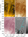 |
Fig. 1. Overview of the coronal loop observed on 2016 March 23. The FOV was observed at about 03:04 UT in AIA 171 Å (a), 193 Å (b), 211 Å (c), and in the HMI LOS magnetic magnetogram (d). The coronal loop of interest is indicated by an arrow in each panel. Within the PFSS magnetic field extrapolation, the magnetic field line that is closely aligned with this loop is overlaid (cyan curve) on the HMI LOS magnetogram. The region of interest used in the DEM analysis is enclosed in the blue rectangle. The evolution of this loop is shown in an online movie. |
The SDO/AIA images that were used in this observation have a cadence of about 12 s, and each pixel corresponds to about 0.6″. The SDO/HMI observes the full-disk photospheric magnetic fields. The AIA images and HMI magnetograms were both calibrated with the standard routines in the Solar SoftWare package (Lemen et al. 2012; Schou et al. 2012).
2.2. Loop geometry
This coronal loop was predominantly detectable in the AIA 171 Å channel, therefore we used the AIA 171 Å images to obtain its geometry. We created a two-dimensional curvilinear coordinate. One curve coordinate was chosen to be aligned with the spine of the coronal loop, and the second coordinate was set to be normal to the coronal loop. We made a bilinear interpolation of the emission intensity in the AIA 171 Å channel into the curvilinear coordinate. Then each intensity profile across the loop was fit with a Gaussian function plus a linear background. In order to improve the signal-to-noise ratio, we averaged three neighboring profiles before fitting. The full width at half-maximum (FWHM) of that Gaussian function was considered as the loop width (w). The fitting error was used as uncertainties of the loop width (e.g., Aschwanden & Boerner 2011; Gupta et al. 2019). The error for the AIA 171 Å intensity was estimated according to the method described by Yuan & Nakariakov (2012).
In Fig. 2a, nine cross cuts were made along the coronal loop and are plotted with the short color lines. Each intensity profile was scaled to a proper range and stacked in Fig. 2b. The loop width was measured at locations perpendicular to the loop axis from the footpoint to the apparent top at a distance of about 130 Mm, as indicated in Fig. 2c. We note that at some positions (e.g., positions close to 8 and 9), the obtained loop widths deviate significantly from those of their neighbors. The reason is that some random bright patchy background contaminated these emission intensity profiles. On the other hand, at some positions of the footpoint (i.e., 1), the loop of interest overlaps some bright closed loops. This resulted in the broad loop widths.
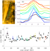 |
Fig. 2. Estimation of the loop width. a) smaller FOV (∼76 Mm × 149 Mm) of the AIA 171 Å image. The loop is highlighted by a green arrow. Nine sample cuts are marked by short lines and are numbered from 1 to 9. b) intensity profiles along the cuts indicated in panel a, normalized by their maximum intensity. The color used in each curve is the same as used in the numbered short lines in panel a. Each profile is elevated progressively for visualization purpose. c) loop width variation along the loop length. The numbers mark the nine loop segments in panel a. |
2.3. DEM analysis
In order to obtain the thermal properties of this loop, we focused on a smaller field of view (FOV), as marked in Fig. 1 and performed a differential emission measure (DEM) analysis. Observations taken from six EUV channels of SDO/AIA (94 Å, 131 Å, 171 Å, 193 Å, 211 Å, and 335 Å) were used to calculate the DEM(T) distribution for each pixel. We used an improved version (Su et al. 2018) of the sparse inversion code (Cheung et al. 2015). The derived solutions provide valuable information by mapping the thermal plasma from 0.3 to 30 MK. The DEM uncertainties were estimated from a Monte Carlo (MC) simulation (Su et al. 2018). Random noise of the observed emission intensity was added to the MC simulation, and the inversion was repeated for 100 times, then the standard deviations of the 100 MC simulations were used as the uncertainties of DEM solutions.
Figures 3a−d draw the EM (Cheung et al. 2015; Su et al. 2018) maps from 0.32 MK to 3.98 MK within which coronal loops are normally detected. These EM maps were calculated from a set of six rebinned AIA narrow-band maps with a pixel size of 1.2″, in order to obtain a clear view of the structures in different temperature ranges, whose emissions are accumulated along the line of sight (LOS) into the observed intensity. The coronal loop was clearly seen in the temperature range of 0.63 MK−1.12 MK (Fig. 3b) and to a lesser extent in the 1.26 MK−2.24 MK range (Fig. 3c). In order to measure the temperature of the coronal loop of interest, we then plotted the DEM profiles (Fig. 3e) of seven positions in the coronal loop. The obtained DEM profiles exhibit two peaks at about 0.8 MK and 1.8 MK. However, the coronal loop of interest was most clearly seen in the DEM ranging from 0.63 MK to 1.12 MK. We therefore assume that the high-temperature peak at about 1.8 MK originated from the emission of the diffuse background in the AIA 211 Å channel. For a comparison, we then took the DEM profile of a reference point (0) in the background for cross-validation (Fig. 3b). We note that the DEM profile in the background indeed only has a prominent peak at about 1.8 MK.
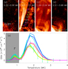 |
Fig. 3. DEM results of the target coronal loop. a–d: narrow-band EM maps integrated in the temperature ranges of 0.32 MK−0.56 MK, 0.63 MK−1.12 MK, 1.26 MK−2.24 MK, and 2.51 MK−3.98 MK. e: DEM profiles at seven selected positions (1−7) along the loop and in one location (0) away from the loop. The color corresponds to the positions labeled in panel b. For clarity, panel e only draws the error bars at loop position 4. The gray region indicates the EM integrated range. |
The EM was calculated by integrating the DEM over temperatures, EM = ∫DEM dT. We only used the temperature ranges between 0.32−1.12 MK. This range is the effective temperature of the coronal loop of interest, as indicated in Fig. 3e. The EM might be considered the product of the square of the number density of electrons (ne) and LOS depth, which might be approximated with the loop width (w). In this way, the electron number density can be calculated with  . Finally, a DEM-weighted mean temperature (such as T = ∫DEM TdT/∫DEM dT) was used to estimate the temperature of this coronal loop. The errors for the density and temperature were also calculated from the 100 MC simulations. These steps were repeated for every pixel along the loop length. Then, using the obtained number density, plasma temperature, and magnetic field, we calculated the plasma beta (β) along the coronal loop.
3. Properties of the coronal loop
3.1. Geometry of the loop
The coronal loop under study was very thin and ultra long. It was detectable for a projected length of about 130 Mm. We note this as a lower limit because it became diffuse and invisible in the background. The loop width was about 1 Mm at the footpoint and expanded to about 1.5 Mm to 2.0 Mm at the visible end. The loop expansion ratio was about 1.5 to 2.0. In this dataset of about 2 h, we observed the distinctive coronal loop to fade out eventually, but it had an almost constant width during its lifetime (see the online movie).
Within the PFSS extrapolation model, we traced a magnetic field line that was closely aligned with the coronal loop of interest, as indicated in Fig. 1d. This magnetic field line was connected to a patch of negative polarity and extended to the outer space. This coronal loop can therefore be regarded as an open structure. It has an inclination in the range of 40 ° −80° based on the estimation in the PFSS model. The polarity at the loop footpoint has an average LOS magnetic field component of about 100 Gauss. Along the field line, the strength of the magnetic field is about 10 Gauss on average, whereas the maximum field strength can reach 60 Gauss. We therefore used 10 Gauss as the field strength of the coronal loop.
3.2. Thermal property of the loop
Figure 3 presents the DEM results to the coronal loop of interest. It is apparent that this loop is most clearly identifiable in the EM map at 0.63 MK−1.12 MK (Fig. 3b). However, each DEM profile of the coronal loop normally has two peaks, one at about 0.8 MK and another at 1.8 MK (Fig. 3e). After a comparison with the background DEM profile, we conclude that the DEM peak at 1.8 MK corresponds to a strong component from the emission of the diffuse background in the 211 Å channel (Fig. 1c). Therefore we estimate that the coronal loop considered here had a temperature of about 0.8 MK.
In Fig. 4 we present the quantitative estimate of the physical parameters of the coronal loop. Figure 4a draws the AIA 171 Å intensity (Yuan & Nakariakov 2012) and EM variations at the selected positions along the loop length. They first decreased quickly with the loop length and then became roughly stable. We note that the AIA 171 Å intensities are much stronger at the beginning, which might be because some random bright patchy or closed loops contaminated the intensity at the base of the coronal loop (see also Figs. 1 and 2).
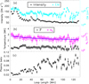 |
Fig. 4. Quantitative estimate of the coronal loop parameters. The EM (a), the emission intensity in the AIA 171 Å bandpass (a), the plasma temperature (b), and the number density of electrons (b), as well as the plasma beta (β) as a function of projected length along the loop. The blue line represents the best-fit result for the number density. |
Figure 4b plots the plasma temperature variation along the loop length. It shows that this coronal loop had a very uniform temperature at (0.7 ± 0.2) MK. This is consistent with our previous estimates. Because this loop was very thin, we cannot obtain the temperature distribution across the loop. Figure 4b also shows the estimated number density of electrons along the loop length, with a mean number density of (8 ± 2) × 108 cm−3. The electron number density was about 1.0 × 109 cm−3 at the footpoint, and dropped off exponentially to around 5 × 108 cm−3 at the end of the loop. This was a stratification pattern. Therefore we fit an exponential function to the density profile and obtained a density scale height of about (38 ± 13) Mm. This scale height only incorporates a reduced gravity because this corona loop is inclined with respect to the solar radius. The theoretical density scale height is (22.8 ± 6.6) Mm for a plasma with a temperature of (0.7 ± 0.2) MK. With the ratio of theoretical and fitted scale heights, we estimate that the loop deviated from the gravity vector on average by an angle of about 54 ° ±30°. This value is consistent with the estimate of the extrapolated magnetic field, that is, 40 ° −80°.
Figure 4c draws the plasma beta parameter (β) as a function of the loop length. This increased from about 0.02 at the footpoint to roughly 0.1 at its visible end. The average plasma beta of this loop is estimated to be ∼0.056 ± 0.037.
4. Conclusion and discussion
We used SDO/AIA data to observe an open coronal loop associated with AR 12524. This coronal loop was clearly detected in AIA 171 Å and to an weaker extent in the AIA 193 Å and 211 Å channels. This loop was ultra long and had a small width. Its lifetime was about 90 min. The loop width was about 1.5 Mm, and the projected length is about 130 Mm. The coronal loop we investigated is thinner and longer than those reported earlier. For instance, Aschwanden & Boerner (2011) reported coronal loops of about 2−4 Mm wide and 10−40 Mm long. Moreover, most loops have a lifetime of about 20−30 min (e.g., Peter & Bingert 2012), whereas in our case, the loop survived for over one hour. The coronal loop had a plasma temperature of (0.7 ± 0.2) MK. No significant variation in temperature was detected along the loop. This loop was relatively cold (e.g., < 1 MK) and was approximately unithermal. This is consistent with spectroscopic and imaging observations (e.g., Del Zanna & Mason 2003; Warren et al. 2008; Tripathi et al. 2009). The electron number density was measured to be about 1.0 × 109 cm−3, and it dropped off exponentially to about 0.5 × 109 cm−3 at the visible end of the loop. This is a stratification pattern. The density scale height was measured to be roughly (38 ± 13) Mm. The plasma beta increased from about 0.02 to roughly 0.1, which means that the gas pressure decreased with height by a smaller amount than the magnetic pressure. More observational, geometrical, and physical parameters of this loop are listed in Table 1.
Observational, geometrical, and physical parameters of the analyzed coronal loop.
A weak expansion like this has been found in many coronal loops at SXR/EUV wavelengths since the era of TRACE and earlier (e.g., Klimchuk et al. 1992; Klimchuk 2000; Watko & Klimchuk 2000; Peter & Bingert 2012; Kucera et al. 2019). These coronal loops were closed structures and often exhibited weak expansion from double footpoints to the loop apex (López Fuentes et al. 2006; Brooks et al. 2007). An open coronal loop of about 280 Mm long was reported by Gupta et al. (2019), but its loop width expanded from 20 Mm at the footpoint to 80 Mm at the loop top. Here, we investigated an ultra-long (∼130 Mm) and very thin (∼1.5 ± 0.5 Mm) coronal loop that did not appear to have undergone significant expansion as it rose above the photosphere.
A very interesting point is that the loop width expanded only by a factor of about 1.5 to 2.0, whereas this loop had a projected length of about three pressure scale heights. The pressure decreased by 95% (i.e., 1 − e−3), therefore the cross section of this loop should have expanded by a factor of about 19. However, this is not supported by the observation. To explain the nearly constant cross section of this coronal loop, there must be unresolved features (e.g., Klimchuk et al. 2000; Petrie 2008). The lifetime of this steady coronal loop is much longer than the timescales of the radiative cooling and thermal conduction. We therefore used a magnetostatic model (Appendix A) to explain the small radial expansion of this loop. We used a thin flux tube approximation and assumed that the magnetic field has a twist term (e.g., Ferriz-Mas & Schüssler 1989). Only when the twist term was large enough did the external pressure become negative. Thus, we were able to set an upper limit for the twist. The detailed derivation process is described in Appendix B. We then constrained the expansion factor to be 1.5 and obtained the solution for the external pressure. To constrain the thin magnetic flux tube, the twist had to be smaller than about 0.65 (see, Fig. B.1). This means that with a sufficiently twisted magnetic field, this coronal loop can be constrained to be at magnetic equilibrium.
When we go beyond magnetostatic equilibrium, this loop has to be supplied with steady flows of mass and energy because we did not observe any features such as propagating emission, intensity, or brightening. This flow must have had a very long lifetime or would have to have occurred intermittently on short timescales. Evidence has been collected that the footpoint of a coronal loop can have an unresolved minority polarity. This is a miniature bipolar field that emerges into a constant background field. This configuration favors small scale magnetic reconnection (Wang et al. 2019). Repeated reconnections provide continuous mass and energy to the coronal loops (Chitta et al. 2018). Unfortunately, we did not observe features to support this scenario, but we note that the AIA instrument might not be sensitive enough to capture these features.
Finally, we stress that the loop widths are measured as the FWHMs of the cross-sectional profiles of the coronal loop detected in the SDO/AIA 171 Å channel. One AIA pixel corresponds to 0.44 Mm (Lemen et al. 2012). A loop width of about 1.5 to 2.0 Mm spans about 4−5 pixels. This measurement is obtained by fitting an intensity profile with about 12 pixels. This practice could reach a higher accuracy than the pixel scale and has been used by many other researchers (e.g., Aschwanden & Boerner 2011; Anfinogentov et al. 2013; Anfinogentov & Nakariakov 2019; Reale 2014).
Movie
Movie of Fig. 1 Access here
Acknowledgments
We acknowledge the anonymous referee for his/her valuable comments. This study is supported by NSFC under grant 11973092, 11803008, 11873095, 11790300, 11790302, 11729301, 11773079, the Youth Fund of Jiangsu No. BK20171108 and BK20191108. The Laboratory No. 2010DP173032. D.L. is also supported by the Specialized Research Fund for State Key Laboratories. D.Y. is supported by the NSFC grant 11803005, 11911530690, Shenzhen Technology Project (JCYJ20180306172239618), and Shenzhen Science and Technology program (group No. KQTD20180410161218820). T.V.D. is supported by the European Research Council (ERC) under the European Union Horizon 2020 research and innovation programme (grant agreement No 724326) and the C1 grant TRACEspace of Internal Funds KU Leuven (number C14/19/089). Y.S. is supported by the NSFC grant U1631242, 11820101002, and the Jiangsu Innovative and Entrepreneurial Talents Program.
References
- Anfinogentov, S. A., & Nakariakov, V. M. 2019, ApJ, 884, L40 [CrossRef] [Google Scholar]
- Anfinogentov, S., Nisticò, G., & Nakariakov, V. M. 2013, A&A, 560, A107 [NASA ADS] [CrossRef] [EDP Sciences] [Google Scholar]
- Aschwanden, M. J., & Boerner, P. 2011, ApJ, 732, 81 [NASA ADS] [CrossRef] [Google Scholar]
- Aschwanden, M. J., & Peter, H. 2017, ApJ, 840, 4 [NASA ADS] [CrossRef] [Google Scholar]
- Bray, R. J., Cram, L. E., Durrant, C., et al. 1991, Plasma Loops in the Solar Corona (Cambridge: Cambridge University Press) [Google Scholar]
- Brooks, D. H., Warren, H. P., Ugarte-Urra, I., et al. 2007, PASJ, 59, S691 [NASA ADS] [CrossRef] [Google Scholar]
- Chastain, S. I., & Schmelz, J. T. 2017, ArXiv e-prints [arXiv:1705.06776] [Google Scholar]
- Chen, F., Peter, H., Bingert, S., et al. 2014, A&A, 564, A12 [NASA ADS] [CrossRef] [EDP Sciences] [Google Scholar]
- Cheung, M. C. M., Boerner, P., Schrijver, C. J., et al. 2015, ApJ, 807, 143 [NASA ADS] [CrossRef] [Google Scholar]
- Chitta, L. P., Peter, H., & Solanki, S. K. 2018, A&A, 615, L9 [NASA ADS] [CrossRef] [EDP Sciences] [Google Scholar]
- Del Zanna, G., & Mason, H. E. 2003, A&A, 406, 1089 [NASA ADS] [CrossRef] [EDP Sciences] [Google Scholar]
- Dudík, J., Dzifčáková, E., & Cirtain, J. W. 2014, ApJ, 796, 20 [CrossRef] [Google Scholar]
- Feng, L., Inhester, B., Solanki, S. K., et al. 2007, ApJ, 671, L205 [NASA ADS] [CrossRef] [Google Scholar]
- Ferriz-Mas, A., & Schüssler, M. 1989, Geophys. Astrophys. Fluid Dyn., 48, 217 [NASA ADS] [CrossRef] [Google Scholar]
- Golub, L., Herant, M., Kalata, K., et al. 1990, Nature, 344, 842 [NASA ADS] [CrossRef] [Google Scholar]
- Goddard, C. R., Pascoe, D. J., Anfinogentov, S., et al. 2017, A&A, 605, A65 [NASA ADS] [CrossRef] [EDP Sciences] [Google Scholar]
- Gupta, G. R., Del Zanna, G., & Mason, H. E. 2019, A&A, 627, A62 [NASA ADS] [CrossRef] [EDP Sciences] [Google Scholar]
- Klimchuk, J. A. 2000, Sol. Phys., 193, 53 [NASA ADS] [CrossRef] [Google Scholar]
- Klimchuk, J. A., Lemen, J. R., Feldman, U., et al. 1992, PASJ, 44, L181 [NASA ADS] [CrossRef] [Google Scholar]
- Klimchuk, J. A., Antiochos, S. K., & Norton, D. 2000, ApJ, 542, 504 [NASA ADS] [CrossRef] [Google Scholar]
- Kucera, T. A., Young, P. R., Klimchuk, J. A., et al. 2019, ApJ, 885, 7 [NASA ADS] [CrossRef] [Google Scholar]
- Lemen, J. R., Title, A. M., Akin, D. J., et al. 2012, Sol. Phys., 275, 17 [Google Scholar]
- Li, L. P., Peter, H., Chen, F., et al. 2015, A&A, 583, A109 [NASA ADS] [CrossRef] [EDP Sciences] [Google Scholar]
- Lionello, R., Winebarger, A. R., Mok, Y., et al. 2013, ApJ, 773, 134 [NASA ADS] [CrossRef] [Google Scholar]
- López Fuentes, M. C., Klimchuk, J. A., & Démoulin, P. 2006, ApJ, 639, 459 [NASA ADS] [CrossRef] [Google Scholar]
- Malanushenko, A., & Schrijver, C. J. 2013, ApJ, 775, 120 [NASA ADS] [CrossRef] [Google Scholar]
- McTiernan, J. M., & Petrosian, V. 1990, ApJ, 359, 524 [NASA ADS] [CrossRef] [Google Scholar]
- Mikić, Z., Lionello, R., Mok, Y., et al. 2013, ApJ, 773, 94 [NASA ADS] [CrossRef] [Google Scholar]
- Peter, H., & Bingert, S. 2012, A&A, 548, A1 [NASA ADS] [CrossRef] [EDP Sciences] [Google Scholar]
- Peter, H., Bingert, S., Klimchuk, J. A., et al. 2013, A&A, 556, A104 [NASA ADS] [CrossRef] [EDP Sciences] [Google Scholar]
- Petrie, G. J. D. 2006, ApJ, 649, 1078 [NASA ADS] [CrossRef] [Google Scholar]
- Petrie, G. J. D. 2008, ApJ, 681, 1660 [NASA ADS] [CrossRef] [Google Scholar]
- Pesnell, W. D., Thompson, B. J., & Chamberlin, P. C. 2012, Sol. Phys., 275, 3 [NASA ADS] [CrossRef] [Google Scholar]
- Poletto, G., Vaiana, G. S., Zombeck, M. V., et al. 1975, Sol. Phys., 44, 83 [NASA ADS] [CrossRef] [Google Scholar]
- Priest, E. R., Foley, C. R., Heyvaerts, J., et al. 1998, Nature, 393, 545 [NASA ADS] [CrossRef] [Google Scholar]
- Reale, F. 2014, Liv. Rev. Sol. Phys., 11, 4 [Google Scholar]
- Schmelz, J. T., & Martens, P. C. H. 2006, ApJ, 636, L49 [NASA ADS] [CrossRef] [EDP Sciences] [Google Scholar]
- Schou, J., Scherrer, P. H., Bush, R. I., et al. 2012, Sol. Phys., 275, 229 [Google Scholar]
- Schrijver, C. J., & De Rosa, M. L. 2003, Sol. Phys., 212, 165 [Google Scholar]
- Su, Y., Veronig, A. M., Hannah, I. G., et al. 2018, ApJ, 856, L17 [CrossRef] [Google Scholar]
- Tripathi, D., Mason, H. E., Dwivedi, B. N., et al. 2009, ApJ, 694, 1256 [NASA ADS] [CrossRef] [Google Scholar]
- Vasheghani Farahani, S., Nakariakov, V. M., & van Doorsselaere, T. 2010, A&A, 517, A29 [NASA ADS] [CrossRef] [EDP Sciences] [Google Scholar]
- Vesecky, J. F., Antiochos, S. K., & Underwood, J. H. 1979, ApJ, 233, 987 [NASA ADS] [CrossRef] [Google Scholar]
- Watko, J. A., & Klimchuk, J. A. 2000, Sol. Phys., 193, 77 [NASA ADS] [CrossRef] [Google Scholar]
- Warren, H. P., Ugarte-Urra, I., Doschek, G. A., et al. 2008, ApJ, 686, L131 [NASA ADS] [CrossRef] [Google Scholar]
- Wang, Y.-M., Ugarte-Urra, I., & Reep, J. W. 2019, ApJ, 885, 34 [CrossRef] [Google Scholar]
- Yuan, D., & Nakariakov, V. M. 2012, A&A, 543, A9 [NASA ADS] [CrossRef] [EDP Sciences] [Google Scholar]
Appendix A: Thin flux tube model
We used a magnetostatic plasma to model the coronal loop of interest. This model accounts for plasma stratification and a static magnetic field. In our case, the loop has a lifetime significantly greater than the timescales of thermal conduction and radiative cooling, therefore we resort to a magnetostatic plasma. This loop has a high aspect ratio (ratio between the loop length and radius). We used the thin flux tube approximation (e.g., Ferriz-Mas & Schüssler 1989) to model the twisted coronal loop. We expanded the magnetohydrodynamic (MHD) quantities for a thin cylindrical flux tube with cylindrical coordinates (r, φ, z). We considered an axisymmetric magnetohydrostatic equilibrium solution to the MHD equations. We assumed a velocity v = 0 and set all time- and φ-derivatives to 0. In particular, we used the following thin flux tube expansion for the loop parameters,

where B = (Br, Bφ, Bz) is the magnetic field, p is the pressure, ρ is the density, and T is the temperature.
We derived the key equations for a thin and twisted flux. We expanded the magnetohydrostatic equations in the radial component, and balanced the forces in the flux tube at a certain distance R(z) with an external pressure force pe(R(z)). The latter relationship is their closure relationship for the (otherwise) infinite system of equations. The resulting equations for the thin and twisted flux tube are

where primes denote the derivative with respective to z, μ is the magnetic permeability, g is the gravity pointing in the negative z-direction, and ℛ is the universal gas constant divided by the molar mass.
Because the radial expansion is of particular importance in our problem, we related it to the magnetic field variables in the problem. The general equation for the flux surface in the (r, z)-plane is
this is not a separable equation. However, when we take Bz2 = 0, as was done in Vasheghani Farahani et al. (2010), the equation becomes

using Eq. (A.8), we find as the solution

where we used the same asterisk notation to indicate the value at a reference height z = 0. This equation expresses the conservation of magnetic flux in a flux tube: as the magnetic field decreases, the radius of the flux tube must increase quadratically.
Appendix B: Solution for an expanding loop
We assumed that the loop radius expands exponentially with height (see also Dudík et al. 2014),
For an expansion factor R(ztop)/R⋆ = η, we find L = ztop/lnη. In particular, we can consider η = 2 or η = 1.5 for the observations and ztop = 130 Mm, then L = 186 Mm or 320 Mm, respectively.
From the conservation of magnetic flux (Eq. (A.15)), we then find
Eq. (A.8) can be used to find the radial component,
and Eq. (A.10) can be integrated (following Ferriz-Mas & Schüssler 1989) to determine the φ-component of the magnetic field:
from Eq. (A.9), we obtain
![$$ \begin{aligned} p_2=-\frac{B_{z0}^2}{\mu }\left[\frac{1}{L^2}+\left(\frac{B_{\varphi 1}^\star }{B_{z0}^\star }\right)^2\right] \exp {(-4z/L)}, \end{aligned} $$](/articles/aa/full_html/2020/07/aa38433-20/aa38433-20-eq21.gif)
this equation shows that p2 < 0, and in particular, the total pressure (p0 + r2p2) is therefore negative beyond a critical radius.
We now assume that we have a constant temperature T0 without radial variation (T2 = 0). From Eq. (A.7), we obtain in this case
where we define the scale height H = ℛT0/g. For a temperature of T0 = 0.7 MK, the scale height is about 22.8 Mm, and this value is increased to 38 Mm when we reduce the gravity by projection.
We then employ Eq. (A.12) to obtain external pressure of the tube pe:
Because R⋆/L is small, the external pressure usually remains positive. Only when the twist term  is large does the external pressure become negative. Thus, we can find an upper limit for the twist (see, Fig. B.1). For an expansion factor of 1.5 (or 2.0), the upper limit of the twist is around 0.65 (or 0.5). These values are compatible with the limits for kink instability.
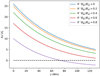 |
Fig. B.1. Profiles of the gas pressure ratio of the external and internal plasma for various twists. |
All Tables
Observational, geometrical, and physical parameters of the analyzed coronal loop.
All Figures
|
Fig. 1. Overview of the coronal loop observed on 2016 March 23. The FOV was observed at about 03:04 UT in AIA 171 Å (a), 193 Å (b), 211 Å (c), and in the HMI LOS magnetic magnetogram (d). The coronal loop of interest is indicated by an arrow in each panel. Within the PFSS magnetic field extrapolation, the magnetic field line that is closely aligned with this loop is overlaid (cyan curve) on the HMI LOS magnetogram. The region of interest used in the DEM analysis is enclosed in the blue rectangle. The evolution of this loop is shown in an online movie. |
| In the text | |
|
Fig. 2. Estimation of the loop width. a) smaller FOV (∼76 Mm × 149 Mm) of the AIA 171 Å image. The loop is highlighted by a green arrow. Nine sample cuts are marked by short lines and are numbered from 1 to 9. b) intensity profiles along the cuts indicated in panel a, normalized by their maximum intensity. The color used in each curve is the same as used in the numbered short lines in panel a. Each profile is elevated progressively for visualization purpose. c) loop width variation along the loop length. The numbers mark the nine loop segments in panel a. |
| In the text | |
|
Fig. 3. DEM results of the target coronal loop. a–d: narrow-band EM maps integrated in the temperature ranges of 0.32 MK−0.56 MK, 0.63 MK−1.12 MK, 1.26 MK−2.24 MK, and 2.51 MK−3.98 MK. e: DEM profiles at seven selected positions (1−7) along the loop and in one location (0) away from the loop. The color corresponds to the positions labeled in panel b. For clarity, panel e only draws the error bars at loop position 4. The gray region indicates the EM integrated range. |
| In the text | |
|
Fig. 4. Quantitative estimate of the coronal loop parameters. The EM (a), the emission intensity in the AIA 171 Å bandpass (a), the plasma temperature (b), and the number density of electrons (b), as well as the plasma beta (β) as a function of projected length along the loop. The blue line represents the best-fit result for the number density. |
| In the text | |
|
Fig. B.1. Profiles of the gas pressure ratio of the external and internal plasma for various twists. |
| In the text | |
Current usage metrics show cumulative count of Article Views (full-text article views including HTML views, PDF and ePub downloads, according to the available data) and Abstracts Views on Vision4Press platform.
Data correspond to usage on the plateform after 2015. The current usage metrics is available 48-96 hours after online publication and is updated daily on week days.
Initial download of the metrics may take a while.