| Issue |
A&A
Volume 639, July 2020
|
|
|---|---|---|
| Article Number | A110 | |
| Number of page(s) | 16 | |
| Section | Interstellar and circumstellar matter | |
| DOI | https://doi.org/10.1051/0004-6361/202037796 | |
| Published online | 20 July 2020 | |
Large-scale [C II] 158 μm emission from the Orion-Eridanus superbubble
Leiden Observatory, Leiden University,
PO Box 9513,
2300 RA
Leiden,
The Netherlands
e-mail: This email address is being protected from spambots. You need JavaScript enabled to view it.
Received:
22
February
2020
Accepted:
29
April
2020
Abstract
In this study, we analyzed the [C II] 158 μm emission from the Orion-Eridanus region measured by the Cosmic Background Explorer. Morphologically, the [C II] emission traces prominent star-forming regions this area. The analysis takes into account five different components of the interstellar medium (ISM) that can contribute to the [C II] emission: compact H II regions, dense Photon-Dominated Region, surfaces of molecular clouds, the Warm Ionized Medium, and the Cold Neutral Medium. We estimate the contribution from each object of interest to the observed [C II] emission based upon the physical properties of the object and validate our results by making a comparison with existing “small” scale maps. Inside the ~400 parsec aperture radius that we investigate, surfaces of molecular clouds exposed to radiation from nearby stellar clusters are the dominant contributor to the observed global [C II] flux. These molecular cloud surfaces are exposed to moderate radiation fields (G0 ~ 100 times the average interstellar radiation field) and are moderately dense (nH ~ 103 cm−3). In addition, extended low-density ionized gas, along with large-scale ionized gas structures (Barnard’s Loop; λ Ori) also make a substantial contribution. The implications of this study for the analysis of extragalactic [C II] observations are assessed.
Key words: ISM: general / local insterstellar matter
© ESO 2020
1 Introduction
The origin of [C II] 158 μm emission from the interstellar medium of galaxies is a widely studied topic, largely driven by the observed tight correlation between [C II] and various star formation tracers (Boselli et al. 2002; de Looze et al. 2011; Herrera-Camus et al. 2015). Many interstellar components may contribute to the [C II] emission observed in regions of massive star formation, including dense photo-dissociation regions, ionized gas in compact H II regions or in the form of the diffuse warm ionized medium (WIM), surfaces of molecular clouds (SfMCs), and nearby diffuse clouds (Cold Neutral Medium (CNM)) (Croxall et al. 2012, 2017; Cormier et al. 2012; Kapala et al. 2015; Abdullah et al. 2017). The emission of each of these depends on the local physical conditions and as each interacts differently with massive stars, the relationship between the observed [C II] luminosity and the star formation activity may vary from region to region. Furthermore, despite the good general correlation between the observed [C II] emission and the star formation activity, given its low ionization potential, [C II] 158 μm emission may also arise from gas which has no direct relationship to star formation activity. Analysis of the observed [C II] emission from well-resolved galactic regions provides a promising method for addressing these issues and a number of studies with different observing strategies have been performed. These range from surveys of small to large, individual objects (Graf et al. 2012; Sandell et al. 2015; Pabst et al. 2017, 2019) to pointed surveys along individual sight-lines (Goldsmith et al. 2012; Pineda et al. 2014; Velusamy & Langer 2014; Velusamy et al. 2015; Langer et al. 2016). While much can be learned by comparison of these observations to tracers of neutral (HI and CO) and ionized gas, it is a non-trivial undertaking to assess the contribution of individual components to the large-scale [C II] emission on a galactic scale.
Here we address these issues by analyzing observations on the scale of an OB association. We have selected the Orion-Eridanus region for this study as it has been studied extensively at a wide variety of wavelengths. The Orion-Eridanus super-bubble lies approximately 5° below the plane which limits confusion with background galactic sources. This complex spans up about 50 degrees on the sky, and its distance ranges from ~300–600 pc (Pogge et al. 1992; Giannini et al. 2000; O’Dell & Henney 2008; Berné et al. 2009; O’Dell & Harris 2010; O’Dell et al. 2011; Graf et al. 2012; Sandell et al. 2015). In Hα, the most conspicuous features of this complex are M 42, M 43, λ Ori, and Barnard’s Loop (Fig. 1). Several well-known molecular clouds (Dame et al. 2001; Mizuno et al. 2003; Planck Collaboration XIII 2014; Nishimura et al. 2015) show up prominently in the Planck 545 GHz map of the dust emission, including the Orion Molecular Clouds A & B (hereafter OMC A & B), the Monoceros R2 cloud (Mon R2), and the λ Ori molecular ring. These clouds are all characterized by ongoing massive star formation as traced, for example, by 12 μm emission.
The Orion-Eridanus region provides a natural template for the study of [C II] 158 μm emission from extragalactic regions of star formation as it is a region of active star formation, individual components are well resolved and have been studied in detail, and the total [C II] 158 μm emission has been measured by COBE (Bennett et al. 1994). We note that, if it were adapted to the distance of a typical galaxy studied by the PACS instrument on the Herschel Space Observatory, the physical scale of the Orion-Eridanus region would be ~12′′, with the beam size of this instrument at 158 μm. The Orion-Eridanus region has been studied extensively in the past (Brown et al. 1995; O’Dell et al. 2011; Bally 2008; Ochsendorf et al. 2015; Goicoechea et al. 2015; Pabst et al. 2019).
This complex harbours a variety of interstellar medium phases (compact H II regions, PDRs, molecular clouds, and diffused ionized gas as well as HI gas) representative of the general ISM in an external galaxies. The ionized gas in this complex has been studied rigorously inHα by O’Dell et al. (2011), Pon et al. (2014) and Ochsendorf et al. (2015). Mizuno et al. (2003) presented a large-scale CO study of this complex. Many more studies were conducted on several smaller scales in this complex, such as Orion Molecular Clouds A and B (Nishimura et al. 2015) and M 42 (Weilbacher et al. 2015).
We organized this paper into seven sections. This introduction is followed by the presentation of the observational data (Sect. 2). In Sect. 3, we analyze the [C II] emission. We discuss our findings in Sect. 4 and compare this study with GOTC+ result in Sect. 5. In Sect. 6, the implication of this study with regard to the extragalactic study of [C II] are presented and we present our conclusions in Sect. 7.
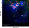 |
Fig. 1 False-color image of the Orion-Eridanus Complex. The blue filter is Hα, tracing ionized gas, taken from the WHAM survey (Haffner et al. 2003), the green filter is the 12 μm map of WISE data (Wright et al. 2010), while the red filter is the Planck 857 GHz map (Planck Collaboration XI 2014). The scale size is 100 pc at the distance of M 42 (414 pc). We labeled some of the ISM gas component present on the aperture. |
2 Observational data
2.1 The [C II] COBE data
The [C II] map is obtained from the Far Infrared Absolute Spectrophotometer (FIRAS) instrument on the Cosmic Microwave Background Explorer (COBE) and has a resolution of 7° (Bennett et al. 1994). The [C II] emission from FIRAS COBE is extracted from a ~ 28 ° aperture (Fig. 2). This aperture has been chosen to include the full Orion-Eridanus superbubble. As the Orion-Eridanus region is well below the galactic plane, the adopted aperture avoids confusion with other galactic emission sources. The extraction aperture – encompassing the Orion-Eridanus superbubble – corresponds to a physical diameter of 440 pc assuming an average distance of 450 pc, which corresponds well to the typical resolution of regions studied in local group galaxies: for example, with a beam size of ~ 12′′, the physical scale size is 400 pc for a local group galaxy located at a distance of ~ 7 Mpc.
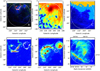 |
Fig. 2 Orion-Eridanus region at different wavelengths. The color scale of these images has been manipulated to make the structures present stand out better. Panel A: overall Orion-Eridanus Region under study. Colors are as in Fig. 1. The [C II] COBE extraction aperture is shown as white circle with a physical extension of ~400 pc, taking 414 pc as average distance. Panel B: FIRAS COBE [C II] map and the extractionaperture as a white circle. Panel C: HI map integrated over the velocity range −40 km s−1 < νLSR < 40km s−1 (Brown et al. 1995). Panel D: CO(J = 2−1) map from Planck. The small white circles cover those parts of the four molecular clouds (Orion Molecular A & B, λ Ori, and Mon R2) and are used in our analysis (see also Figs. 4–6). Panel E: WIM extraction aperture for Barnard’s Loop and λ Orionis. The small white circles covering these two objects identify the apertures over which we performed our analysis. Panel F: extraction aperture of M 42 from Pogge et al. (1992) is shown in white circle. Each panel has different scale size. |
2.2 Ancillary data
We make use of the all sky survey Hα map from Finkbeiner (2003) composed of the Virginia Tech Spectral-line Survey (Dennison et al. 1998), the Southern H-alpha Sky Survey Atlas (Gaustad et al. 2001), and the Wisconsin H α Mapper (WHAM) (Haffner et al. 2003) data. The HI map is obtained from the Leiden-Argentine-Bonn (LAB) survey (Kalberla et al. 2005). The 12 μm map is obtained from Wide-Field InfraRed Survey (WISE), (Wright et al. 2010), the 25, 60, and 100 μm maps are obtained from Improved Reprocessing of the IRAS Survey (IRIS) a new generation of Infrared Astronomical Satellite (IRAS) images (Miville-Deschênes & Lagache 2005). Planck maps at 217, 353, 545, and 857 GHz were also employed to construct the SED of the Orion-Eridanus complex (Planck Collaboration XI 2014). All of the maps are convolved to the H α resolution of 6′ using a Gaussian kernel from Aniano et al. (2011).
In order to model the [C II] emission from specific objects within the larger COBE beam, we broke the observed emission structure in the Hα and CO maps using the small apertures indicated in Fig. 2. For the compact H II region, M 42, we adopted the aperture used in Pogge et al. (1992). For Hα, these apertures cover the relevant structures visible in the map. For the Orion Molecular Clouds (OMC) A and B, we limited ourselves to those parts of the clouds that are coincident with the bright emission in the COBE [C II] map.
2.3 Morphological comparison
In Fig. 3, we compare the morphology of [C II] FIRAS COBE with several gas tracer (see Sect. 2.2): The H α map from the WHAM survey, the CO(J = 2−1) emission from Planck, HI from the LAB survey, as well as the dust emission tracers: WISE 12 μm, IRAS 25 and 100 μm, 857 GHz from Planck. We also compare the [C II] COBE morphology with the location of the young stellar population in Fig. 3. We overplot the locations of bright O and B stars in Fig. 3. Lee & Chen (2009) and Zari et al. (2017) have shown that the stellar clusters have ages between 1 and 15 Myr where the Orion Nebula Cluster is the youngest stellar cluster (1–2 Myr old) and the 25 Ori cluster is the oldest (13–15 Myr).
The COBE [C II] map has a resolution of 7° (Bennett et al. 1994). At the average distance of Orion-Eridanus complex, ~450 pc, this angular resolution correspond to a physical size of 50 pc. Hence, fine details such as M 42 or NGC 2024 are not resolved in the COBE [C II] map. We summarize our finding of the [C II] emission morphology below.
We recognize three [C II] components in the Orion Eridanus region (Fig. 3). The first and brightest [C II] emission arises from the Orion Complex. The second brightest [C II] component is the λ Ori complex. These two components account for ≃60% of the observed [C II] emission from this region. The remainder is in a diffuse component which is not directly associated with molecular clouds or active regions of star formation. As we argue later, we associate this diffuse [C II] emission component with extreme low-density ionized gas (the so-called ELDWIM). We discuss the modeling aspect with regards to these three distinct components in Sect. 4.2.
The main peak in the [C II] emission of the Orion-Eridanus region resembles the 100 μm IRAS map of the dust emission. The COBE spatial resolution is insufficient to separate the contributions from the two main regions of massive star formation, M 42 and NGC 2024. Neither the H α nor the HI map resembles the [C II] map.
The overall agreement between the [C II] emission morphology and the IRAS 100 μm map tracing warm dust heated by far-ultraviolet photons from the massive stars supports the hypothesis that the main [C II] excitation mechanism is through the photoelectric heating process which links the dust heating process with the gas heating process (Tielens & Hollenbach 1985; Bakes & Tielens 1994; Okada et al. 2013).
The Orion molecular clouds A and B stand out clearly in the CO(J = 2−1) map obtained by Planck as well as the sub-millimeter dust continuum maps. These latter trace high column density of cold material shielded from the direct FUV stellar light. The molecular clouds extend much beyond the peak in the [C II] emission in the Orion-Eridanus region.
From this comparison, we conclude that the peaks in the [C II] emission trace the direct interaction of massive stars with their environment (Fig. 3). This emission extends to the closest surface of molecular clouds enveloping the star-forming region. We quantify this conclusion in our modeling of [C II], where we show that the [C II] emission arises mainly from components with moderate strength of G0, close to the star-forming region (see Sect. 3).
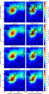 |
Fig. 3 Morphological comparison of [C II] COBE with several continuum and gas tracers. The [C II] emission is shown as color-coded contour. The white dots represent the O and B stars. |
3 [C II] emission from the Orion-Eridanus region
The Orion-Eridanus region is complex and a number of different components can contribute to the observed [C II] emission. We estimate theindividual contribution of these components with simple models, using physical conditions determined from a variety of observations. We compare these estimates – where possible – to resolved observations to assess their validity. We will then compare theestimates for the different components with each other and with the total observed flux in the Orion-Eridanus region.
3.1 The [C II] COBE observations
The total observed [C II] FIRAS COBE flux inside this aperture is 3.1 × 10⁻⁶ erg s−1 cm−2 or a luminosity ~2.3 × 1036 erg s−1 (~ 2 × 10⁴ L⊙). The Orion-Eridanus complex has an angular size of 3.0 steradians. The observable surface brightness of [C II] is then 1.0 × 10⁻⁶ erg s−1 cm−2 sr−1. The observed, average, [C II] surface brightness of the Orion-Eridanus complex is an order of magnitude smaller than the typical [C II] surface brightness from extragalactic H II regions observed in the KINGFISH program by the PACS instrument on the Herschel Space Observatory (Kennicutt et al. 2011; Croxall et al. 2012; Abdullah et al. 2017), but is comparable to that observed for weaker members of the class of dwarf galaxies (Cigan et al. 2016). With only a very limited number of massive stars, Orion is a wimpy region of massive star formation that only stands out in our sky because of its proximity and because it is well isolated below the galactic plane. The extragalactic regions targeted in, for example, the KINGFISH program contain richer star clusters or several Orion-like star-forming regions closely packed within the beam. However, this COBE [C II] flux (3.1 × 10⁻⁶ erg s−1 cm−2) is still within the detection limit of the PACS instrument (3 × 10⁻¹⁵ erg s−1 cm−2 5 σ in 1 h).
Characteristics of the various components present in the Orion-Eridanus region.
3.2 Compact H II regions
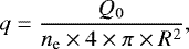
To calculate the [C II] emission from compact H II regions, we have to make an ionization correction as only a small fraction of the carbon is in the form of C+. We used the Modeling And Prediction in PhotoIonised Nebulae and Gas-dynamical Shocks (MAPPINGS) tool (Dopita et al. 2000) to calculate the expected [C II] emission from all compact H II regions within the Orion-Eridanus region. The two main parameters that are needed to model the [C II] emission are the electron density, ne, and the ionization parameter, q. The latter is given by Eq. (1),
 (1)
(1)
where Q0 is the number of Lyman Continuum Photons and R is the size of the H II region. The compact H II regions included in our analysis are M 42, M 43, IC434, Monocerotis R2, and NGC 2024. The characteristics of these regions are summarized in Table 1. For M 42 we use the [SII]6717 over [SII]6731 ratio from Pogge et al. (1992) to determine the electron density. We obtain a gas density of 3 × 103 cm−3. The ionization parameter is calculatedby adopting Q0 ~ 1048.87 photons s−1 (O’Dell et al. 2017) and a radiusof ~0.4 pc. We scale the calculated [C II]/Hβ ratio to the observed Hβ flux (Pogge et al. 1992) to obtain the model [C II] flux (see Table 2). M43 is a smaller H II regions located adjacent to the M 42 separated only by a dark lane of dust. For this region, we adopt the results from the literature for the physical conditions: an electron density of ~500−600 cm−3 (Rodríguez 1999, 2002; O’Dell & Harris 2010; Simón-Díaz et al. 2011), a total ionizing photon luminosity, Q0 = 1047.2 photons s−1 (Simón-Díaz et al. 2011) and a size of 0.65 pc (Simón-Díaz et al. 2011). We obtain an ionization parameter log q = 6.9 log(cm s−1) typical for small H II regions. We scaled the modeled [C II]/Hα ratio from MAPPINGS to the observed Hα flux (Simón-Díaz et al. 2011) (see Table 2).
For the H II region IC 434 we use the region characteristic obtained by Ochsendorf & Tielens (2015). The ionization parameter is derived in similar manner as in M 43. The central star (σ Ori) has an ionizing photon luminosity of Q0 = 1047.88 photons s−1 (Martins et al. 2005). The ionization parameter is evaluated at the ionization front at a distance of ≃4 pc from the central star. We take the average density of IC 434 to be ~100 cm−3 (Ochsendorf & Tielens 2015). We then use MAPPINGS to calculate the [C II] surface brightness relative to H α, given the above gas condition, and scaled this to the total Hα flux observed by WHAM (Hα ~ 5.2 × 10⁻⁹ erg s−1 cm−2 from Ochsendorf et al. 2014, see Table 2).
There has been a long standing debate on the ionizing star of NGC 2024 as this region is highly obscured by dust (Bik et al. 2003). Bik et al. (2003) argue that IRS2b is the main ionizing star with a spectral type of O8. The number of Lyman Continuum Photons that is radiated by an O8 star is Q0 = 1048.29 photons s−1 (Martins et al. 2005). We take the size of this H II region to be ~0.2 pc and adopt a density of ne = 1500 cm−3 from Giannini et al. (2000) to calculate the ionization parameter (Table 1). The [C II] flux was then determined analogously to that for M 43 and IC 443 (Table 2).
The last H II region in this complex is the ultra compact H II region, Monocerotis R2. We adopt the H II region properties from Downes et al. (1975) and Jaffe et al. (2003). The ne and q parameter are then calculated accordingly (Table 1). As this source is highly obscured, we cannot use optical emission lines to scale the [C II] flux. Instead, we have used the observed [NeII] 12.8 μm flux ~5.7 × 10⁻¹⁰ erg s−1 cm−2 (Jaffe et al. 2003).
The H II region in IC 434 is the only region where the [C II] emission from the ionized gas has been directly measured. For this region, the calculated [C II] surface brightness is in good agreement with the observations(Table 2). For M 42, Goicoechea et al. (2015) estimate that a maximum of 10% of the observed [C II] emission arises from the H II region our prediction agree with this result. We note that the contributionof dense ionized gas to the global [C II] flux of the Orion-Eridanus region is small (Table 2).
[C II] modeling result.
3.3 Dense PDRs
The [C II] emission from dense PDRs is governed by two important parameter: the incident radiation field, G0, and the gas density, nH. For all of the dense PDRs in the Orion-Eridanus complex we use the central ionizing star parameter to derive G0. We follow the relation below from Tielens (2005),
 (2)
(2)
where L is the total luminosity of central star in solar luminosity, R is the distance from the star in pc, and G0 is in units of the average interstellar radiation field (Habing 1968).
M 42 is ionized by θ1 Ori C (O’Dell et al. 2017) with a bolometric luminosity of 2.0 × 10⁵ L⊙ (Simón-Díaz et al. 2006). Following Goicoechea et al. (2015) and Salgado et al. (2016), we adopt 0.4 pc for the distance of the star to the PDR. This results in a G0 of 2.6 × 10⁴. In M 43 the ionizing star is NU Ori, a B0.5V star (O’Dell & Harris 2010). The stellar bolometric luminosity is calculated based on the stellar models of Vacca et al. (1996). The distance between the star and the PDR is estimated from the observed optical size of the H II region (0.65 pc; Simón-Díaz et al. 2006). For NGC 2024 we adopt the luminosity of an O8 type star (Vacca et al. 1996) appropriate for IRSb2 (Giannini et al. 2000; Bik et al. 2003). The physical size of NGC 2024 PDR is obtained from [C II] observations (Graf et al. 2012). In IC 434, the distance of the illuminating star, σ Ori, to the PDR surface is adopted from the work of Ochsendorf & Tielens (2015) and we use the stellar characteristic from Lee (1968) and Ochsendorf & Tielens (2015). The reflection nebula, NGC 2023, is the 5th PDR to consider. It has been studied in detail by Steiman-Cameron et al. (1997), Sheffer et al. (2011), and Sandell et al. (2015). Much of the [C II] emission arises from low-density (nH ~ 750 cm−3) material (Steiman-Cameron et al. 1997) rather than the prominent dense ridge to the southeast of the star. For simplicity, we adopt the gas condition from Sheffer et al. (2011), G0 = 9 × 10³ and nH = 500 cm−3. For the size of the PDR, we adopt the size of the [C II] observation (~220′′; Sandell et al. 2015). The last dense PDR considered in this region is the dense PDR associated with the ultra compact H II region, Monocerotis R2. We take the dense PDR properties from the study of Berné et al. (2009). The size of Monocerotis dense PDR is taken from the [C II] observation of Ossenkopf et al. (2013) to be ~0.04 pc.
The densities of the PDRs associated with H II regions are all derived assuming pressure equilibrium between the neutral and ionized gas. The adopted densities of the ionized gas for these regions have been discussed in Sect. 3.2. We assume a typical temperature for the ionized gas in M 42 of 8000 K (Weilbacher et al. 2015)and 7000 K for the other regions (O’Dell & Harris 2010). For the PDR we assume a temperature of 300 K. The dense PDR properties are summarized in Table 1. We use the PDR model from Kaufman et al. (2006) and Pound & Wolfire (2008) to estimate the [C II] surface brightness from dense PDRs given the G0 and nH in Table 1. For M 42, M 43, and IC 434, we use the radius where G0 is evaluated toconvert the [C II] surface brightness to the [C II] flux.
Each of these PDRs has been observed partially or fully at high spatial resolution. Here, we compare our model calculations with these observations (Table 2). For M 42, the modeled surface brightness is lower by factor of three than the observed one. The observed [C II] surface brightness is very high compared to to any model for face-on PDRs and may reflect the importance of geometry (for example edge-on for the Orion Bar) or a too small adopted linewidth in the models. For the PDRs in IC 434 and NGC 2023, both the calculated surface brightnessesand the fluxes are in good agreement with the observations. We note again that for the latter source, the [C II] emission is dominated by the low-density material (Steiman-Cameron et al. 1997). In Mon R2, the calculated surface brightness and flux are somewhat higher than observed. Likely, this region is somewhat less dense than adopted. For NGC 2024, the model overestimates the observed surface brightness and flux by factor of 2, presumably, because the density is actually somewhat lower than adopted. Overall, the agreement is satisfactory.
We note that the total [C II] emission from the 1 pc2 region associated with the dense PDRs surrounding the Trapezium cluster is ~173 L⊙ (Goicoechea et al. 2015). This value corresponds to < ~1% of the total [C II] emission inside our COBE aperture. Hence, this study supports our modeling result that dense PDRs with high G0 and high nH contribute relatively little to the large-scale [C II] emission from regions such as the Orion-Eridanus complex.
[C II] modeling per selected region.
3.4 Surface of molecular clouds
There are four conspicuous molecular clouds structures in the Orion-Eridanus complex as shown in Figs. 1 and 2. The dominant molecular clouds are the Orion Molecular Clouds A and B. The third molecular cloud in the Orion-Eridanus complex is the bubble structure surrounding the H II regions associated with λ Ori, and the last is the Monocerotis R2 molecular cloud. We have covered these molecular clouds with a set of circular apertures with sizes ranging from 2 × 10⁻⁴ to 3 × 10⁻³ sr where we limit ourselves to those parts of the cloud that are bright in the far infrared as those will dominate the [C II] emission (Figs. 2, 4–6). As the incident radiation field varies considerably even over this selected set, we estimate the [C II] emission from molecular cloud surfaces in the Orion-Eridanus region by modeling each of these areas separately and then summing their contribution.
The strength of [C II] emission from molecular clouds is governed by G0 and nH as this component is a PDR in physical sense. We made use of the IRAS (60 and 100 μm) and Planck (217, 353, 545, and 857 GHz) data to construct SED and obtained the Td (Planck Collaboration XIII 2014). We then converted Td to G0 using the following relation based on Hollenbach et al. (1991):
 (3)
(3)
where Td is dust temperature in K. The G0 derived for the different regions in these molecular clouds range between ~ 1−102 with a typical value of 10 (Tables 4–6).
For the density, we adopt the result from Nishimura et al. (2015) for OMC A and B nH ≃ 1000 cm−3. The gas density for Mon R2 is assumed to be similar to OMC A and B. For the molecular clouds surrounding λ Ori, we adopt the density from Goldsmith et al. (2016), nH ~ 200 cm−3. Based on these two parameters (G0 and nH) we derived the [C II] surface brightness from PDR models (Kaufman et al. 2006; Pound & Wolfire 2008). The expected flux from molecular cloud surfaces is then calculated by multiplying each calculated surface brightness by the aperture size and summing these up to arrive at the total [C II] flux from SfMCs in the Orion-Eridanus region. The results are summarized in Tables 4–6.
Goldsmith et al. (2016) has measured the [C II] surface brightness for L1599, one dark cloud in the λ Ori molecular ring, to be 9 × 10⁻⁶ erg s−1 cm−2 sr−1. This observation coincides with region 13 in our analysis (see Table 5 and Fig. 5) with a modeled surface brightness of 2.85 × 10⁻⁵ erg s−1 cm−2 sr−1 about three times higher than observed. For low UV fields, the [C II] surface brightness is not sensitive to the density in PDR models as it is the dominant cooling line of the gas. However, we note that the G0 derived from Td is much higher than the observed total FIR surface brightness would indicate and, concomitantly, the derived averaged dust optical depth is very small (Table 5). We interpret this as a small filling factor of the molecular cloud in the aperture analyzed. This would imply that we overestimate the [C II] flux as well.
For OMC A and B, as these clouds are large on the sky, there is only limited data to compare with our calculations. For the Orion A molecular cloud, the average intensity has been determined for a ~1 square degree region centered on the trapezium stars to be 1.3 × 10⁻⁴ erg s−1 cm−2 sr−1 (Stacey et al. 1993; Pabst et al. 2019). These observations coincide with region I in our aperture. The modeled surface brightness for this region is ~2.2 erg s−1 cm−2 sr−1, in reasonable agreement with the observations (Table 4). We note that the regions within ~3 pc of the ionizing stars of M 42 and NGC 2024 contribute significantly (≃50%) to the modeled [C II] flux from the surfaces of molecular clouds.
OMC A and B [C II] modeling.
3.5 Warm ionized medium
In Hα, the Orion-Eridanus region shows two major structures, Barnard’s Loop and the nebula surrounding λ Ori. We show in Fig. 2 the set of circular aperture used to extract the WIM component of Orion-Eridanus complex [C II] emission. We adopt the electron density for Barnard’s Loop from O’Dell et al. (2011) with ne = 3.2 and 2 cm−3 for λ Ori (Sahan & Haffner 2016). For sanity check we take the line ratios of [N II] 122 and 205 μm to H α inside the COBE aperture choosing only pixels with high signal-to-noise ratio (S/N). The observed [N II]122 over H α ~ 1.13 and [N II]205 over Hα ~ 0.08. Indeed both values give estimates of density in the low-density limit with upper limit of 10 cm−3 as given by [N II]205 over Hα ratio.
As the observed gas density is lower than the critical density (nc = 44 cm−3) of [C II] emission in ionized gas we scale the [C II] emission directly from H α. Following Heiles (1994), we calculate the [C II] over Hα ratio,
 (4)
(4)
where we have adopted a gas phase C+ abundance equal to the total gas phase C abundance (Sofia et al. 1997) and we have used the deexcitation collision coefficient summarized by Goldsmith et al. (2012). The results are given in Table 2.
The observations reveal excess Hα flux within our aperture which cannot be accounted for by the identifiable ionized gas structures. This excess constitutes a significant (≃ 0.62, FHα = 1.8 × 10⁻⁶ erg s−1 cm−2) fraction of the total observed H α flux inside the COBE aperture. To distinguish this extra Hα emission from the regions above, we call this Extremely Low Density Warm Ionized gas (ELDWIM). We assume thatthe density of this component is less than the [C II] critical density and then scale the inferred H α flux directlyto the expected [C II] flux (Eq. (4); Table 1) and temperature of 8000 K.
3.6 Cold neutral medium
We use the HI observation of the LAB survey (Kalberla et al. 2005). We integrated the HI column from νLSR ~ −40 km s−1 to 40 km s−1 (Brown et al. 1995). Wolfire et al. (1995) have developed detailed models for the CNM phase of the ISM in pressure and thermal equilibrium. These models provide the [C II] flux per H-atom for the CNM. This flux depends on the ambient interstellar radiation field, The results of the Planck Collaboration Int. XXIX (2016) provide a G0 of ≃1 and the Wolfire et al. (1995) models give then a [C II] flux of 2.7 × 10⁻²⁶ erg s−1perH-atom. This value is in good agreement with studies of the [C II] emission from diffuse atomic clouds (Wolfire et al. 1995). We have adopted this value to convert the observed HI column densities into [C II] fluxes (Table 2). There are no direct observations of [C II] emission from CNM components in the Orion-Eridanus region that can be used to validate this value but a comparison to estimates based upon both measurements of UV absorption lines (Gry et al. 1992) and sounding rocket experiments (Bock et al. 1993) lends confidence to the results.
λ Ori molecular ring [C II] modeling.
Mon R2 molecular clouds [C II] modeling.
4 Results and discussions
4.1 The energy budget in the Orion-Eridanus complex
In our 400 pc aperture, most of the gas and dust heating occur close to the location of the two main molecular clouds of OMC A and B (see Figs. 2 and 4). The main mechanism of gas heating is gas ionization by young stellar populations which are concentrated on the bright rim of OMC A and B as shown in H α map (Figs. 2 and 4). The IRAS map reveal that most of the dust emission also originates from close to these active regions of massive star formation, but they lack the spatial resolution to narrow this down further.
In OMC A, the most active star-forming region is the Orion Nebula Cluster, which harbours ~10 OB stars centered on M 42 (Hillenbrand 1997; Lee & Chen 2009). The total H α emission in the 440 pc aperture is ~7 × 1037 erg s−1 or 1.8 × 10⁴ L⊙. This Hα luminosity is at the low end of H II regions and associations commonly studied in external galaxies such as M 51, NGC 3521, NGC 3627, or NGC 4736 (Kennicutt et al. 1989). In addition, as discussed in Sect. 3.5, most of the H α emission is associated with a diffuse ionized gas (WIM) component and the distinct and localized Barnard’s Loop and λ Ori ring structures rather than the compact H II regions. We construct the Spectral Energy Distribution (SED) for the whole Orion-Eridanus region from IRAS 60, and 100 μm, and Planck 217, 353, 545, and 857 GHz maps. The SED in Fig. 8 shows a rather cold dust temperature of 18 K with β value of 1.56 (Lombardi et al. 2014; Pabst et al. 2017). The integrated FIR radiation from 60 to 1300 μm is ~1.4 × 10⁻⁴ erg s−1 cm−2 which translates into LFIR ≃ 8.5 × 10⁵ L⊙. Our LFIR estimation agrees with the result from Ochsendorf et al. (2015). The total Lyman continuum luminosity inside the COBE aperture is 1.1 × 10⁵ L⊙ (Ochsendorf et al. 2015). The Lyman continuum luminosity traces the stellar radiation absorbed by the gas (ionizing hydrogen) rather than the dust while LFIR measures the total energy from the stars as much of the cooling radiation of the (ionized) gas eventually winds up heating the dust as well. We can compare the observed [C II] luminosity with the observed LFIR to derive the heating efficiency of the neutral gas. The gas heating efficiency is a measure of the fraction of the UV luminosity of the stars that winds up heating the gas rather than the dust through the photo-electric effect. The observed heating efficiency for the total aperture is ɛ ≃ 2.2 × 10⁻². This heating efficiency exceeds the average value measured for the whole galaxy by COBE (3 × 10⁻³; Bennett et al. 1994) by an order of magnitude and is somewhat larger than the heating efficiency measured for dense PDRs such as the Orion Bar, NGC 2023 (ɛ ≃ 10−2; Hollenbach & Tielens 1997). and the molecular cloud, L1630, illuminated by σ Ori (G0 ≃ 100; ɛ ≃ 10−2; Pabst et al. 2017). Thus, it seems that the conditions in the Orion-Eridanus region are very conducive to coupling the stellar photons to the gas thermal reservoir. This difference in the heating efficiency between the Orion-Eridanus region may partly reflect that surfaces of molecular clouds are characterized by a relatively large G0 /nH ratio and this results in high efficiency of the photo-electric effect (Bakes & Tielens 1994). In addition, the Orion-Eridanus region may have a relatively large contribution to the [C II] emission by diffuse ionized gas (cf., Table 2) as compared to the whole galaxy. Finally, we note that a substantial fraction of the IR emission of the galaxy as a whole is powered by relatively cool stars emitting predominantly visible photons that do not ionize PAHs or small dust grains and hence do not couple to the gas.
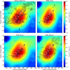 |
Fig. 4 Close-up morphological comparison between [C II] COBE to Planck CO(J = 2−1), WISE 12 μm, IRAS 25 and100 μm on Orion Molecular Clouds complex. Several young stellar cluster are marked with blue circle. Among them are Orion Nebula Cluster, NGC 1977, NGC 1980, NGC 1981, NGC 2024, NGC 2071, NGC 2068. The green dot marks the region studied by Pabst et al. (2017). White large circles mark the aperture used to extract the parameter in Table 4. |
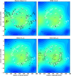 |
Fig. 5 Close-up morphological comparison between [C II] COBE to Planck CO(J = 2−1), WISE 12 μm, IRAS 25 and100 μm on λ Ori molecular clouds complex. The blue star symbol is λ Ori. The white circles are the aperture used to extract the parameter listed in Table 5. |
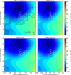 |
Fig. 6 Close-up morphological comparison between [C II] COBE to Planck CO(J = 2−1), WISE 12 μm, IRAS 25 and100 μm on Monocerotis R2. The white circles are the aperture used to extract the properties in Table 6. |
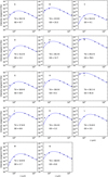 |
Fig. 7 Spectral energy distribution of region plotted in Fig. 4. We fit the IRAS 60 and 100 μm, and the fourPlanck continuum observation. |
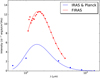 |
Fig. 8 Spectral energy distribution of the area inspected in this study. The aperture size is ~ 28° which translates to ~400 pc in physical size. The 60, and 100 μm m data points are from IRAS, the rest of the points are from Planck (217, 353, 545, and 857 GHz). |
4.2 The overall [C II] emission budget of the Orion-Eridanus complex
We tabulate the estimated [C II] emission from each of the physical components – as derived in Sect. 3 – in Table 2. The total modeled [C II] flux is 4.8 × 10⁻⁶ erg s−1 cm−2 in good agreement with the total observed [C II] emission inside the COBE aperture (3.1 × 10⁻⁶ erg s−1 cm−2).
Several studies, using the high spectral resolution SOFIA/upGREAT instrument, have pointed out that the [C II] line is often optically thick and shows self absorption effects (Graf et al. 2012; Mookerjea et al. 2018, 2019; Guevara et al. 2020). High optical depth are also revealed by the detection of the [13 CII] line profile observed towards several dense PDRs (for example M 43, Horsehead Nebula, and MonocerotisR2) in the Eridanus-Superbuble as reported by Guevara et al. (2020). Typical C+ column densities in dense PDRs are 1018 C+ atoms/cm2 (Hollenbach et al. 1991; Sternberg & Dalgarno 1995; Kaufman et al. 1999). With a line width of 3 km s−1 and a temperature of 300 K, the [C II] 158 μm optical depth in the PDR to the nearest surface is ≃1 and potentially very large in edge-on geometries. In the energy balance and emergent intensity calculation, self-absorption by the PDR itself is taken into account in PDR models in the Sobolov approximation (c.f., Tielens & Hollenbach 1985).
While this is a local approximation, detailed studies show that this provides results for the integrated intensity and cooling accurate to 10% (Elitzur & Asensio Ramos 2006). Of course, the conversion of the observed [C II] 158 μm line to a mass of C+ emitting gas is more uncertain. Our modeling for dense PDRs (specifically, the three regions: M 43, IC 434, and Monocerotis R2) reveals that they make only small contributions to the total [C II] emission (see Table 2) reflecting the physical conditions and the small solid angle these regions occupy in the COBE beam. Hence we can safely assume that [C II] self-absorption has minimal effect on this assessment. The effect of foreground absorption by the general diffuse ISM can be assessed from the HI data. The total HI column density towards Orion-Eridanus Superbubble is obtained by integrating LAB data from − 400 km s−1 < νLSR < −40 km s−1, which yields NH = 9.3 × 1018 cm−2. Taking an abundance ratio of C to H of C/H = 1.4 × 10⁻⁴ (Sofia et al. 1997) we obtain  of 1.3 × 1015 cm−2. This column density corresponds to an optical depth τ([CII]) of ≃ 0.001 with a line width of 10 km s−1. Hence, foreground absorption by the general diffuse ISM is also not important for any of the components seen towards the Orion-Eridanus region. We note that, as for dense PDRs, the [C II] emission expected from diffuse clouds in the CNM will, to first order, not be affected by self-absorption. In essence, the [C II] line is the dominant coolant and the temperature of the clouds has to adjust until the cooling balances the gas heating. To assess the effect on the calculation for the WIM, we take the case of Barnard’s Loop with ne = 3.2 cm−3 and typical size of ~7 pc (Ochsendorf & Tielens 2015). The hydrogen column density is then NH = 6.8 × 1019 cm−2. Assuming the same C over H abundance ration, we obtain
  of 9.5 × 1015 cm−2. Assuming that the gas has a velocity width of 10 km s−1, we obtain an optical depth of ≃0.07 and the [C II] emission is optically thin. For molecular cloud surfaces, we expect a C+ column density of 2.6 × 1017 cm−2, corresponding to an optical depth of ≃0.2. However, again, the [C II] line is the dominant coolant of this UV-heated surface layer and the effect on the total (observed or calculated) [C II] emission will be small.
As the Orion-Eridanus superbubble is well out of the plane, absorption by foreground gas in the diffuse ISM is minimal. For extragalactic observations of regions of massive star formation in the galactic plane, a higher column density might be more appropriate. If we adopt a surface density in the CNM typical for the solar neighbourhood of ≃ 2 M⊙ pc−2, we arrive at an optical depth of ≃0.002. Hence, we do not expect that analysis of the [C II] 158 μm line from galaxies is much affected by absorption.
We found from our analysis that the surfaces of molecular clouds (SfMCs), mainly OMC A and B, make the largest contributionto the [C II] flux even though the surface brightness from this component is smaller by an order of magnitude than dense PDRs. This low surface brightness of SfMCs is compensated for by the large beam filling factor of this component. Dense PDRs typically have sizes of less than 0.5 pc, while the illuminated surfaces of molecular clouds have sizes of ≃10 pc. Given the gas parameter in Table 1, we derive a modeled [C II] emission of 3.8 × 10⁻⁶ erg s−1 cm−2 which corresponds to 80% of the modeled [C II] emission. Within this component, the main contribution originates from regions I and F, which are located closest to the young star cluster. The Orion Nebula Cluster is the main ionizing cluster for region I while region F is dominated by NGC 2024. Inside the 7 pc radius adopted for these regions, the dust temperature is ~30 and 29 K which translates to G0’s of ~90 and 80, respectively (Fig. 7). We have adopted densities of ~1000 cm−3 but the model surface brightness is not very sensitive to density in the range ≃ 102−104 cm−3. Each of these regions contributes ≃50% of the modeled [C II] from their molecular cloud (i.e., OMC A and B).
By necessity, regions with moderate incident radiation fields have to lie within ≃ 10 pc of the region of star formation. This intimate connection to massive stars guarantees that the [C II] emission traces the recent star-forming activity in the region. This conclusion is in line with previous observational studies that demonstrate that [C II] emission traces the star formation rate (Boselli et al. 2002; de Looze et al. 2011; Herrera-Camus et al. 2015).
There is a noticeable contribution (≃25%) to the total observed [C II] emission from diffuse ionized gas. The main contribution arises from ELDWIM+WIM component that seems to pervade this region in the WHAM observations. In contrast, the [C II] emission from compact H II regions and their associated PDRs, such as M 42, M 43, and NGC 2023, as well as from the CNM is only of minor (≃5%) importance.
4.3 The [C II] emission from the individual sources in the Orion-Eridanus complex
The COBE observations reveal the presence of two distinct emission regions, associated with the OMC A & B star formation actvity and with the λ Ori bubble. In addition, there is a diffuse emission component – not directly associated with star formation activity – present as well. Here, we will compare the modeled [C II] emission with observation for each of these sources. We list the observed [C II] emission for each of these sources in Table 3. The Orion complex consists of H II and PDR regions of M 42, M 43, IC343, NGC 2023, NGC 2024, OMC A, and OMC B. The λ Ori complex consists of molecular rings and ionized gas. The diffuse component consists of CNM, ELDWIM, and Barnard’s loop.
The modeled [C II] flux for the OMC A and B star-forming regions and for the λ Ori complex are about a factor of two higher than the observed [C II] flux. This emission mainly originates from molecular cloud surfaces illuminated by moderate G0’s. In contrast, the [C II] emission from the diffuse component is slightly underestimated. This emission mainly arises from diffuse ionized gas rather than Barnard’s Loop.
5 Comparison to the GOTC+ galactic survey
It may be ofsome interest to compare our results on an in-depth study of the [C II] emission from the Orion-Eridanus superbubble to that of the galactic survey with Heterodyne Instrument for The Far Infrared (HIFI) Herschel, The Galactic Observations of Terahertz C+ (GOTC+) (Pineda et al. 2013; Goldsmith et al. 2015; Langer et al. 2016). The GOTC+ Open Time Key Project studied the [C II] emission on a galactic scale by surveying 520 pinhole sight-lines with the HIFI instrument on the Herschel Space Observatory. This data was combined with various ancillary data to determine the relative contributions of ionized gas, PDRs, CO-dark H2 gas, and HI clouds to the observed emission. These sight-lines were located in the galactic plane and line-of-sight confusion was addressed through detailed comparison of velocity resolved line profiles. This analysis revealed that typically ~47% of the [C II] emission originates from dense PDRs (G0 = 6–20; nH = 103 -104), 20 and 30% are associated with cold atomic and CO-dark H2 gas, respectively. Ionized gas made only a very small contribution to the observed [C II] emission (Pineda et al. 2013).
The large contribution to the [C II] emission by moderately dense molecular gas illuminated by moderately strong FUV fields is in good agreement with our analysis for the Orion-Eridanus region, albeit that the derived conditions are somewhat different. As much of the diffuse cold neutral gas has been moved to the superbubble walls by the supernova activity in the Orion-Eridanus region, the small contribution of HI in our analysis as compared to the GOTC+ analysis is, perhaps, not so surprising. The inferred small contribution of ionized gas to the [C II] flux observed by GOTC+ may reflect that diffuse ionized gas that dominates this type of emission in Orion-Eridanus would have been missed by that survey. Indeed, the ionized gas that contributes to the observed [C II] emission by GOTC+ and its offspring surveys has an inferred much higher electron density (~30 cm−3; Goldsmith et al. 2015).
6 The Orion-Eridanus region as a template for extra-galactic observation
6.1 Estimating the [C II] emission from 10 Mpc
In this section, we analyze the [C II] emission from the Orion-Eridanus region assuming it originates from a region that observations cannot resolve; for example, a region of massive star formation in a galaxy at a distance of, say, 10 Mpc (400 pc at 10 Mpc corresponds to ≃8′′, well below the spatial resolution of PACS/Herschel). Several methods to analyze extragalactic [C II] have been reported in the literature (Croxall et al. 2012, 2017; Röllig et al. 2012; Kapala et al. 2015; Abdullah et al. 2017). They all rely on postulating the presence of multiple emission components – PDRs, H II regions, CNM, WIM, and surfaces of molecular cloud – and estimating the contributions of each component using detailed models constrained by ancillary data. We will follow here Abdullah et al. (2017) – but other methods will provide similar results – and analyze the COBE [C II] observations (and all the ancillary data) integrated over the beam. We compare the results of this analysis with the results of our detailed analysis presented inSect. 3 and summarized in Tables 2 and 7 to assess the reliability of conclusions derived of “unresolved” measurements. We start the analysis by considering the [C II] emission from the CNM that is relatively independent of the beam size. For the CNM, we have converted the total HI column density within the beam into the expected [C II] flux using the results on the [C II]/H-atom ratio calculated by models for the ISM (Wolfire et al. 1995). This is completely analogous to the discussion in Sect. 3.6.
For the H II region component, the optical flux will combine the emission from dense H II regions with that from low-density ionized gas. At a distance of 10 Mpc, seeing limited observation with an optical telescope such as KPNO will resolve a physical size of ~50 pc. If one uses an aperture size of 50 pc to extract the H II region a bias toward low-density gas will enter the model as some of the optical emission rises from this low-density ionized gas.
In this analysis, we add the observed fluxes of the ionized gas lines of M 42, Barnard’s Loop, and λ Ori, using data from Pogge et al. (1992), O’Dell et al. (2011) and Sahan & Haffner (2016) (see Appendix A). We then determine the ionizing photon luminosity and the scale size. Using MAPPINGS to model the observed line ratios, we then estimate the density, ne and ionization parameter, q. From the best fit model, we can then derive the [C II] flux expected from the ionized gas. In our analysis, the derived ne decreases from 3.4 × 10⁴ to 1 cm−3 as we add the low-density component and this increases the modeled [C II] emission from 5.7 × 10⁻¹¹ to 1.9 × 10⁻⁷ erg s−1 cm−2. While this mix of low-density and high-density ionized gas greatly increases the [C II] flux from ionized gas, the total contribution is still only ~1/3 of the emission estimated from the ELDWIM (Table 7).
In order to get the actual [C II] emission associated with the ELDWIM, deep integration at H α or radio wavelengths are required over the [C II] aperture. With an ionization potential of 14.5 eV, [N II] emission has to originate from ionized gas. In compact H II regions, N is typically doubly ionized. Moreover, these two fine-structure lines have relatively low critical densities (nc[NII]205 = 45 cm−3 and nc[NII]122 = 280 cm−3, Tielens 2010) compared to other commonly used density tracers, such as [SII]6717 and [SII]6731, and hence trace low-density gas better.
The [N II] IR fine structure lines have, therefore, often been used to estimate the contribution of WIM-like ionized gas to the observed [C II] emission. Both [N II] fine-structure lines (205 and 122 μm) have been observed by COBE/FIRAS and observed fluxes are 1.7 × 10⁻⁶ and 1.2 × 10⁻⁷ erg s−1 cm−2, respectively. The observed ratio of these two lines (≃13.2) which is in the regime where collisional de-excitation occurs hence we can not infer density from this ratio. Given our analysis in Sect. 3.5, we ascribe the [N II] emission to Barnard’s, λ Ori, and ELDWIM. With a [C II] surface brightness of 2.5 × 10⁻⁷ erg s−1 cm−2 sr−1 predicted based upon the Hα surface brightness, the very extended ELDWIM is too faint to be detected by COBE.
The calculated [C II]/[N II] 205 μm ratio is ≃5, which is not very sensitive to the actual density (Abdullah et al. 2017). Hence, the [C II] flux from low-density ionized gas that emits the [N II] lines is ≃6 × 10⁻⁷ erg s−1 cm−2. This value match our estimation based upon the Hα flux.
For the dense PDR component, the dependency on the scale size arises from the determination of G0 and nH. The radiation field incident on the PDR depends on the distance between the ionizing star (cluster) and the PDR surface, which is typically adopted to be the size of the H II region as measured in H α (Abdullah et al. 2017). As the compact H II regions in Orion are much smaller (≤ ~0.5 pc) than the resolution of optical observations (~50 pc at 10 Mpc), this procedure seriously underestimates the incident radiation field on the dense PDRs. Specifically, we arrive at an estimated G0 of 10 rather than 104 as appropriate for the dense PDR in M 42 (Goicoechea et al. 2015). Indeed, this value is more characteristic for the our estimate of the average UV field incident on surfaces of molecular clouds (Sect. 3.4). The low value of G0 is expected as the H II regions in this complex have lower UV luminosity (by one to three orders of magnitude) compared to the regions inspected in Paper 1.
The density in the PDR is then estimated assuming pressure equilibrium between the ionized gas and the PDR. In this procedure, the ionized gas density is taken from the ionized gas analysis and temperatures of Te = 7500 K for the ionized gas and TPDR = 100 K for the PDR are assumed. We adopt the lower limit of H II region density and obtained nH ~200 cm−3. Based on the gas properties derived the definition of dense PDR in this section describes rather surface of molecular clouds than typical dense PDR.
The surface area occupied by such PDR is the last parameter needed. This is by far the most uncertain parameter. This is often estimated from fits to the observed spectral energy distribution of the dust, using the dust model of Draine et al. (2007). This procedure determines the parameter, fPDR, which is the fraction of LFIR that arises from regions with G0 ≥ 100. The SED has been derived from the Planck Collaboration Int. XXIX (2016) and results in fPDR ~ 0.02 for the Orion-Eridanus complex. However our estimated G0 is ~10 which is lower than the cut-off value of 100. Hence using the fPDR from dust model is a bit problematic for wimpy region such as Orion-Eridanus complex where the G0 estimation is lower than expected. Another way to estimate the [C II] is by taking the G0 ~ 100 from the cut-off value of the dust model. Such a PDR component yields [C II] emission of 7.7 × 10⁻⁶ erg s−1 cm−2 which is by a factor of two larger than the observed [C II].
Analogous to the discussion in Sect. 3.4, we estimate the [C II] from SfMCs using PDR models to derive the [C II] over CO J = 2−1 surface brightness ratio and then scaling with the observed CO J = 2−1 flux. In this procedure, we calculate G0 from the dust temperature derived from the observed Orion-Eridanus complex SED (Fig. 8) using Eq. (3), obtaining G0 ~ 5. The density of the molecular clouds is taken from Battisti & Heyer (2014), nH = 500 cm−3. The modeled [C II] emission from SfMCs is then 8.0 × 10⁻⁷ erg s−1 cm−2. This is considerably less than derived in Sect. 3.4.
In our “resolved” analysis, we conclude that the average [C II] emission from SfMCs is a compromise between the value of the average incident radiation field and the scale size of the emitting region. Half of the calculated [C II] emission originated from two, relatively small areas illuminated by G0 ≃ 102. The other half of the [C II] emission came from a much larger surface area illuminated by G0 ≃ 10 − 20. Very little emission originates from molecular cloud surfaces characterized by G0 < 10 (compare also Fig. 5). In contrast, the CO J = 2−1 emission is not very sensitive to the strength of the incident radiation field. Hence, the CO(J = 2−1) flux has limited predictive value for the [C II] flux.
Comparison of [C II] modeling.
6.2 Summary
In summary, the Orion-Eridanus complex is a typical H II region with total H α luminosity in the order of 7 × 1037 erg s−1. Both the optical and the [C II] emission from Orion-Eridanus complex-like regions will be easily detected at a distance of 10 Mpc. However, the ISM properties will be averaged over the beam and this influences the interpretation on the origin of the [C II] emission. Considering the ionized gas, the Hα flux has a large contribution from diffuse ionized gas, while the optical, collisionally excited lines originate from compact HII regions. Modeling reveals then that the inferred properties of the ionized gas are a somewhat ill-defined average of these two components. For Orion-Eridanus, the inferred [C II] flux greatly exceeds the emission from compact H II regions but is only 1/3 of the emissionexpected from the ELDWIM component. For dense PDRs, the average conditions derived from, for example, dust SED modeling lead to a gross overestimate of the [C II] emission from dense PDRs. Our analysis also shows that the contribution from surfaces of molecular clouds cannot be reliably estimated from the observed CO flux as the latter mostly originates from surfaces irradiated by quite low UV fields while the [C II] emission is dominated by surfaces illuminated by moderately strong UV fields.
We demonstrated that more than 80% of [C II] emission in Orion-Eridanus complex rises from molecular clouds exposed to medium strength G0 ~100. Such regions have to be located within ~10 pc from an OB star cluster such as ONC or NGC 2024 and, hence, probe the current star-forming activity. Our result also reveal that a significant (≃20% of the [C II] emission arises from a diffuse, low-density, ionized gas component with no association to the massive stars in the region. Both of these contributions are powered by short-lived massive stars and, hence, our results support earlier studies that the [C II] emission will correlate with the star formation rate. For molecular cloud surfaces, the conversion of the observed [C II] flux to the SFR rate will depend on the photo-electric effect coupling FUV stellar photons to the gas thermal bath as well as the spatial relationship of the molecular gas to the massive stars in the region (i.e., a compromise between surface covering factor and the strength of the incident radiation field). In contrast, the conversion of the [C II] flux originating from ELDWIM regions to a star formation rate will depend on the fraction of ionizing photons “escaping” the immediate, dense environments of the massive stars (i.e., the compact HII region). As these factors may well vary from one region of massive star formation to another, this will introduce scatter in the [C II] emission-star formation rate relation.
7 Conclusions
In this study, we analyze the origin of the [C II] emission in one of the best-studied regions in Milky Way, the Orion-Eridanus complex. The Orion-Eridanus complex is an ideal test bed to resolve the issue of multi-component modeling of [C II] emission as the many regions inside this complex have well-known properties. In addition, relevant objects in Orion-Eridanus complex are located at comparable distances and are relatively free from background contamination by other regions of [C II] emission. ISM components in our models include: 1. H II region, 2. Dense PDR, 3. WIM, 4. SfMCs, 5. CNM. We have used multiwavelength observations from MUSE, COBE, Planck, WISE, LAB HI, IRAS, and the WHAM survey to assist in our analysis. The large-scale of the [C II] COBE map provides an opportunity to simulate [C II] emission from extragalactic regions.
We have compared the results of our model analysis with observations of relevant objects within the region. The good agreement between the model and these observations validates our approach. Overall, the model compares to the global, observed [C II] emission within a factor of 2, which is quite successful given the complexity of the ISM. We further validate our results by examining the [C II] emission from two distinct regions (the Orion complex and the λ Ori complex) as well as with a diffuse emission component revealed by the observations. Here too, the reasonable agreement between calculated and observed fluxes leads credence to our analysis.
We list our important findings below:
-
Morphologically, the bulk of the observed [C II] emission correlates better with the WISE 12 μm, IRAS 25 and 100 μm emission rather than with Planck CO(J = 2−1) and the observed [C II] emission arises from regions where molecular cloud surfaces are exposed to moderate incident radiation fields (G0 ≃ 10−102) produced by nearby, young OB associations.
-
More than half of observed [C II] emission arises from the Orion and the λ Ori complex.
-
Surfaces of molecular clouds are the dominant contributor to the [C II] emission from this region, contributing up to 80% of the total [C II] emission.
-
Our models reveal that 50% of the [C II] emission from surfaces of molecular clouds originates in regions with G0 ~ 100 and are located within 6 pc from young OB star clusters (i.e., the Orion Nebula Cluster and NGC 2024).
-
A substantial (≃0.2) fraction of the observed [C II] emission originates from ELDWIM with electron densities less than 10 cm−3.
-
Dense PDRs and WIM contribute less than 10% to the [C II] emission, while compact H II regions and CNM contribute only ~1% of the observed [C II] emission.
-
Diffuse [C II] makes up a significant (25%) fraction of the observed [C II] emission.
-
Interpretations of distant [C II] observation need to be performed with extra caution.
The study of [C II] emission from Orion-Eridanus complex is a stepping stone in understanding the origin of this emission both for galactic andextragalactic observation. Analysis of large-scale studies such as this [C II] COBE map provides much insight in model studies of the[C II] emission and, in addition, allows us to mimick extragalactic observations. Further large-scale studies are required to assess how typical the Orion-Eridanus complex is as compared to the rest of the galaxy.
Acknowledgements
We acknowledge the use of the Legacy Archive for Microwave Background Data Analysis (LAMBDA), part of the High Energy Astrophysics Science Archive Center (HEASARC). HEASARC/LAMBDA is a service of the Astrophysics Science Division at the NASA Goddard Space Flight Center.
Appendix A Modeling several ionized components
We present the data used in Sect. 6.1 to model ionized component if Orion-Eridanus complex observed in the distance of 10 Mpc. There are three ionized components which dominate the optical flux. These are M 42, λ Ori, and Barnard’s Loop. We add the flux of each components and model this flux.
Sahan & Haffner (2016) has only three emissions for λ Ori, H α, [SII]6717, and [NII]6584. To complete the modeling we add other optical lines such as [OII]3727, [OIII]5007, [SII]6717, and [NII]6548 from MAPPINGS.
Optical flux.
References
- Abdullah, A., Brandl, B. R., Groves, B., et al. 2017, ApJ, 842, 4 [NASA ADS] [CrossRef] [Google Scholar]
- Aniano, G., Draine, B. T., Gordon, K. D., & Sandstrom, K. 2011, PASP, 123, 1218 [NASA ADS] [CrossRef] [Google Scholar]
- Bakes, E. L. O., & Tielens, A. G. G. M. 1994, ApJ, 427, 822 [NASA ADS] [CrossRef] [Google Scholar]
- Bally, J. 2008, Handbook of Star Forming Regions, ed. B. Reipurth (San Francisco: ASP), 459 [Google Scholar]
- Battisti, A. J., & Heyer, M. H. 2014, ApJ, 780, 173 [NASA ADS] [CrossRef] [EDP Sciences] [Google Scholar]
- Bennett, C. L., Fixsen, D. J., Hinshaw, G., et al. 1994, ApJ, 434, 587 [CrossRef] [Google Scholar]
- Berné, O., Fuente, A., Goicoechea, J. R., et al. 2009, ApJ, 706, L160 [NASA ADS] [CrossRef] [Google Scholar]
- Bik, A., Lenorzer, A., Kaper, L., et al. 2003, A&A, 404, 249 [NASA ADS] [CrossRef] [EDP Sciences] [Google Scholar]
- Bock, J. J., Hristov, V. V., Kawada, M., et al. 1993, ApJ, 410, L115 [NASA ADS] [CrossRef] [Google Scholar]
- Boselli, A., Gavazzi, G., Lequeux, J., & Pierini, D. 2002, A&A, 385, 454 [NASA ADS] [CrossRef] [EDP Sciences] [Google Scholar]
- Brown, A. G. A., Hartmann, D., & Burton, W. B. 1995, A&A, 300, 903 [NASA ADS] [Google Scholar]
- Cigan, P., Young, L., Cormier, D., et al. 2016, AJ, 151, 14 [NASA ADS] [CrossRef] [Google Scholar]
- Cormier, D., Lebouteiller, V., Madden, S. C., et al. 2012, A&A, 548, A20 [NASA ADS] [CrossRef] [EDP Sciences] [Google Scholar]
- Croxall, K. V., Smith, J. D., Wolfire, M. G., et al. 2012, ApJ, 747, 81 [NASA ADS] [CrossRef] [Google Scholar]
- Croxall, K. V., Smith, J. D., Pellegrini, E., et al. 2017, ApJ, 845, 96 [NASA ADS] [CrossRef] [Google Scholar]
- Dame, T. M., Hartmann, D., & Thaddeus, P. 2001, ApJ, 547, 792 [NASA ADS] [CrossRef] [Google Scholar]
- de Looze, I., Baes, M., Bendo, G. J., Cortese, L., & Fritz, J. 2011, MNRAS, 416, 2712 [Google Scholar]
- Dennison, B., Simonetti, J. H., & Topasna, G. A. 1998, PASA, 15, 147 [NASA ADS] [CrossRef] [Google Scholar]
- Dopita, M. A., Kewley, L. J., Heisler, C. A., & Sutherland, R. S. 2000, ApJ, 542, 224 [NASA ADS] [CrossRef] [Google Scholar]
- Downes, D., Winnberg, A., Goss, W. M., & Johansson, L. E. B. 1975, A&A, 44, 243 [NASA ADS] [Google Scholar]
- Draine, B. T., Dale, D. A., Bendo, G., et al. 2007, ApJ, 663, 866 [NASA ADS] [CrossRef] [Google Scholar]
- Elitzur, M., & Asensio Ramos, A. 2006, MNRAS, 365, 779 [Google Scholar]
- Finkbeiner, D. P. 2003, ApJS, 146, 407 [NASA ADS] [CrossRef] [Google Scholar]
- Gaustad, J. E., McCullough, P. R., Rosing, W., & Van Buren, D. 2001, PASP, 113, 1326 [NASA ADS] [CrossRef] [Google Scholar]
- Giannini, T., Nisini, B., Lorenzetti, D., et al. 2000, A&A, 358, 310 [NASA ADS] [Google Scholar]
- Goicoechea, J. R., Teyssier, D., Etxaluze, M., et al. 2015, ApJ, 812, 75 [NASA ADS] [CrossRef] [Google Scholar]
- Goldsmith, P. F., Langer, W. D., Pineda, J. L., & Velusamy, T. 2012, ApJS, 203, 13 [Google Scholar]
- Goldsmith, P. F., Yıldız, U. A., Langer, W. D., & Pineda, J. L. 2015, ApJ, 814, 133 [NASA ADS] [CrossRef] [Google Scholar]
- Goldsmith, P. F., Pineda, J. L., Langer, W. D., et al. 2016, ApJ, 824, 141 [CrossRef] [Google Scholar]
- Graf, U. U., Simon, R., Stutzki, J., et al. 2012, A&A, 542, L16 [NASA ADS] [CrossRef] [EDP Sciences] [Google Scholar]
- Gry, C., Lequeux, J., & Boulanger, F. 1992, A&A, 266, 457 [NASA ADS] [Google Scholar]
- Guevara, C., Stutzki, J., Ossenkopf-Okada, V., et al. 2020, A&A, 636, A16 [CrossRef] [EDP Sciences] [Google Scholar]
- Habing, H. J. 1968, Bull. Astron. Inst. Netherlands, 19, 421 [Google Scholar]
- Haffner, L. M., Reynolds, R. J., Tufte, S. L., et al. 2003, ApJS, 149, 405 [NASA ADS] [CrossRef] [Google Scholar]
- Heiles, C. 1994, ApJ, 436, 720 [NASA ADS] [CrossRef] [Google Scholar]
- Herrera-Camus, R., Bolatto, A. D., Wolfire, M. G., et al. 2015, ApJ, 800, 1 [NASA ADS] [CrossRef] [Google Scholar]
- Hillenbrand, L. A. 1997, AJ, 113, 1733 [NASA ADS] [CrossRef] [Google Scholar]
- Hollenbach, D. J., & Tielens, A. G. G. M. 1997, ARA&A, 35, 179 [NASA ADS] [CrossRef] [Google Scholar]
- Hollenbach, D. J., Takahashi, T., & Tielens, A. G. G. M. 1991, ApJ, 377, 192 [NASA ADS] [CrossRef] [Google Scholar]
- Jaffe, D. T., Zhu, Q., Lacy, J. H., & Richter, M. 2003, ApJ, 596, 1053 [NASA ADS] [CrossRef] [Google Scholar]
- Kalberla, P. M. W., Burton, W. B., Hartmann, D., et al. 2005, A&A, 440, 775 [NASA ADS] [CrossRef] [EDP Sciences] [Google Scholar]
- Kapala, M. J., Sandstrom, K., Groves, B., et al. 2015, ApJ, 798, 24 [Google Scholar]
- Kaufman, M. J., Wolfire, M. G., Hollenbach, D. J., & Luhman, M. L. 1999, ApJ, 527, 795 [NASA ADS] [CrossRef] [Google Scholar]
- Kaufman, M. J., Wolfire, M. G., & Hollenbach, D. J. 2006, ApJ, 644, 283 [NASA ADS] [CrossRef] [Google Scholar]
- Kennicutt, Jr. R. C., Keel, W. C., & Blaha, C. A. 1989, AJ, 97, 1022 [NASA ADS] [CrossRef] [Google Scholar]
- Kennicutt, R. C., Calzetti, D., Aniano, G., et al. 2011, PASP, 123, 1347 [NASA ADS] [CrossRef] [Google Scholar]
- Langer, W. D., Goldsmith, P. F., & Pineda, J. L. 2016, A&A, 590, A43 [NASA ADS] [CrossRef] [EDP Sciences] [Google Scholar]
- Lee, T. A. 1968, ApJ, 152, 913 [NASA ADS] [CrossRef] [Google Scholar]
- Lee, H.-T., & Chen, W. P. 2009, ApJ, 694, 1423 [NASA ADS] [CrossRef] [Google Scholar]
- Lombardi, M., Bouy, H., Alves, J., & Lada, C. J. 2014, A&A, 566, A45 [NASA ADS] [CrossRef] [EDP Sciences] [Google Scholar]
- Martins, F., Schaerer, D., & Hillier, D. J. 2005, A&A, 436, 1049 [NASA ADS] [CrossRef] [EDP Sciences] [Google Scholar]
- Miville-Deschênes, M.-A., & Lagache, G. 2005, ApJS, 157, 302 [NASA ADS] [CrossRef] [Google Scholar]
- Mizuno, N., Aoyama, H., Onishi, T., Mizuno, A., & Fukui, Y. 2003, ASP Conf. Ser., 287, 47 [Google Scholar]
- Mookerjea, B., Sandell, G., Vacca, W., Chambers, E., & Güsten, R. 2018, A&A, 616, A31 [NASA ADS] [CrossRef] [EDP Sciences] [Google Scholar]
- Mookerjea, B., Sandell, G., Güsten, R., et al. 2019, A&A, 626, A131 [Google Scholar]
- Nishimura, A., Tokuda, K., Kimura, K., et al. 2015, ApJS, 216, 18 [NASA ADS] [CrossRef] [EDP Sciences] [Google Scholar]
- Ochsendorf, B. B., & Tielens, A. G. G. M. 2015, A&A, 576, A2 [NASA ADS] [CrossRef] [EDP Sciences] [Google Scholar]
- Ochsendorf, B. B., Cox, N. L. J., Krijt, S., et al. 2014, A&A, 563, A65 [NASA ADS] [CrossRef] [EDP Sciences] [Google Scholar]
- Ochsendorf, B. B., Brown, A. G. A., Bally, J., & Tielens, A. G. G. M. 2015, ApJ, 808, 111 [NASA ADS] [CrossRef] [Google Scholar]
- O’Dell, C. R., & Harris, J. A. 2010, AJ, 140, 985 [CrossRef] [Google Scholar]
- O’Dell, C. R., & Henney, W. J. 2008, AJ, 136, 1566 [NASA ADS] [CrossRef] [Google Scholar]
- O’Dell, C. R., Ferland, G. J., Porter, R. L., & van Hoof, P. A. M. 2011, ApJ, 733, 9 [NASA ADS] [CrossRef] [Google Scholar]
- O’Dell, C. R., Kollatschny, W., & Ferland, G. J. 2017, ApJ, 837, 151 [NASA ADS] [CrossRef] [Google Scholar]
- Okada, Y., Pilleri, P., Berné, O., et al. 2013, A&A, 553, A2 [NASA ADS] [CrossRef] [EDP Sciences] [Google Scholar]
- Ossenkopf, V., Röllig, M., Neufeld, D. A., et al. 2013, A&A, 550, A57 [NASA ADS] [CrossRef] [EDP Sciences] [Google Scholar]
- Pabst, C. H. M., Goicoechea, J. R., Teyssier, D., et al. 2017, A&A, 606, A29 [NASA ADS] [CrossRef] [EDP Sciences] [Google Scholar]
- Pabst, C., Higgins, R., Goicoechea, J. R., et al. 2019, Nature, 565, 618 [NASA ADS] [CrossRef] [Google Scholar]
- Pineda, J. L., Langer, W. D., Velusamy, T., & Goldsmith, P. F. 2013, A&A, 554, A103 [NASA ADS] [CrossRef] [EDP Sciences] [Google Scholar]
- Pineda, J. L., Langer, W. D., & Goldsmith, P. F. 2014, A&A, 570, A121 [NASA ADS] [CrossRef] [EDP Sciences] [Google Scholar]
- Planck Collaboration XI. 2014, A&A, 571, A11 [NASA ADS] [CrossRef] [EDP Sciences] [Google Scholar]
- Planck Collaboration XIII. 2014, A&A, 571, A13 [NASA ADS] [CrossRef] [EDP Sciences] [Google Scholar]
- Planck Collaboration Int. XXIX. 2016, A&A, 586, A132 [NASA ADS] [CrossRef] [EDP Sciences] [Google Scholar]
- Pogge, R. W., Owen, J. M., & Atwood, B. 1992, ApJ, 399, 147 [NASA ADS] [CrossRef] [Google Scholar]
- Pon, A., Johnstone, D., Bally, J., & Heiles, C. 2014, MNRAS, 441, 1095 [NASA ADS] [CrossRef] [Google Scholar]
- Pound, M. W., & Wolfire, M. G. 2008, ASP Conf. Ser., 394, 654 [Google Scholar]
- Rodríguez, M. 1999, A&A, 351, 1075 [NASA ADS] [Google Scholar]
- Rodríguez, M. 2002, A&A, 389, 556 [NASA ADS] [CrossRef] [EDP Sciences] [Google Scholar]
- Röllig, M., Simon, R., Güsten, R., et al. 2012, A&A, 542, L22 [NASA ADS] [CrossRef] [EDP Sciences] [Google Scholar]
- Sahan, M., & Haffner, L. M. 2016, AJ, 151, 147 [Google Scholar]
- Salgado, F., Berné, O., Adams, J. D., et al. 2016, ApJ, 830, 118 [NASA ADS] [CrossRef] [Google Scholar]
- Sandell, G., Mookerjea, B., Güsten, R., et al. 2015, A&A, 578, A41 [NASA ADS] [CrossRef] [EDP Sciences] [Google Scholar]
- Sheffer, Y., Wolfire, M. G., Hollenbach, D. J., Kaufman, M. J., & Cordier, M. 2011, ApJ, 741, 45 [NASA ADS] [CrossRef] [Google Scholar]
- Simón-Díaz, S., Herrero, A., Esteban, C., & Najarro, F. 2006, A&A, 448, 351 [NASA ADS] [CrossRef] [EDP Sciences] [Google Scholar]
- Simón-Díaz, S., García-Rojas, J., Esteban, C., et al. 2011, A&A, 530, A57 [NASA ADS] [CrossRef] [EDP Sciences] [Google Scholar]
- Sofia, U. J., Cardelli, J. A., Guerin, K. P., & Meyer, D. M. 1997, ApJ, 482, L105 [NASA ADS] [CrossRef] [Google Scholar]
- Stacey, G. J., Jaffe, D. T., Geis, N., et al. 1993, ApJ, 404, 219 [CrossRef] [Google Scholar]
- Steiman-Cameron, T. Y., Haas, M. R., Tielens, A. G. G. M., & Burton, M. G. 1997, ApJ, 478, 261 [NASA ADS] [CrossRef] [Google Scholar]
- Sternberg, A., & Dalgarno, A. 1995, ApJS, 99, 565 [NASA ADS] [CrossRef] [Google Scholar]
- Tielens, A. G. G. M. 2005, The Physics and Chemistry of the Interstellar Medium (Cambridge: Cambridge University Press) [CrossRef] [Google Scholar]
- Tielens,A. 2010, The Physics and Chemistry of the Interstellar Medium (Cambridge: Cambridge University Press) [Google Scholar]
- Tielens, A. G. G. M., & Hollenbach, D. 1985, ApJ, 291, 722 [NASA ADS] [CrossRef] [Google Scholar]
- Vacca, W. D., Garmany, C. D., & Shull, J. M. 1996, ApJ, 460, 914 [NASA ADS] [CrossRef] [Google Scholar]
- Velusamy, T., & Langer, W. D. 2014, A&A, 572, A45 [NASA ADS] [CrossRef] [EDP Sciences] [Google Scholar]
- Velusamy, T., Langer, W. D., Goldsmith, P. F., & Pineda, J. L. 2015, A&A, 578, A135 [NASA ADS] [CrossRef] [EDP Sciences] [Google Scholar]
- Weilbacher, P. M., Monreal-Ibero, A., Kollatschny, W., et al. 2015, A&A, 582, A114 [NASA ADS] [CrossRef] [EDP Sciences] [Google Scholar]
- Wolfire, M. G., Hollenbach, D., McKee, C. F., Tielens, A. G. G. M., & Bakes, E. L. O. 1995, ApJ, 443, 152 [Google Scholar]
- Wright, E. L., Eisenhardt, P. R. M., Mainzer, A. K., et al. 2010, AJ, 140, 1868 [Google Scholar]
- Zari, E., Brown, A. G. A., de Bruijne, J., Manara, C. F., & de Zeeuw, P. T. 2017, A&A, 608, A148 [NASA ADS] [CrossRef] [EDP Sciences] [Google Scholar]
All Tables
All Figures
|
Fig. 1 False-color image of the Orion-Eridanus Complex. The blue filter is Hα, tracing ionized gas, taken from the WHAM survey (Haffner et al. 2003), the green filter is the 12 μm map of WISE data (Wright et al. 2010), while the red filter is the Planck 857 GHz map (Planck Collaboration XI 2014). The scale size is 100 pc at the distance of M 42 (414 pc). We labeled some of the ISM gas component present on the aperture. |
| In the text | |
|
Fig. 2 Orion-Eridanus region at different wavelengths. The color scale of these images has been manipulated to make the structures present stand out better. Panel A: overall Orion-Eridanus Region under study. Colors are as in Fig. 1. The [C II] COBE extraction aperture is shown as white circle with a physical extension of ~400 pc, taking 414 pc as average distance. Panel B: FIRAS COBE [C II] map and the extractionaperture as a white circle. Panel C: HI map integrated over the velocity range −40 km s−1 < νLSR < 40km s−1 (Brown et al. 1995). Panel D: CO(J = 2−1) map from Planck. The small white circles cover those parts of the four molecular clouds (Orion Molecular A & B, λ Ori, and Mon R2) and are used in our analysis (see also Figs. 4–6). Panel E: WIM extraction aperture for Barnard’s Loop and λ Orionis. The small white circles covering these two objects identify the apertures over which we performed our analysis. Panel F: extraction aperture of M 42 from Pogge et al. (1992) is shown in white circle. Each panel has different scale size. |
| In the text | |
|
Fig. 3 Morphological comparison of [C II] COBE with several continuum and gas tracers. The [C II] emission is shown as color-coded contour. The white dots represent the O and B stars. |
| In the text | |
|
Fig. 4 Close-up morphological comparison between [C II] COBE to Planck CO(J = 2−1), WISE 12 μm, IRAS 25 and100 μm on Orion Molecular Clouds complex. Several young stellar cluster are marked with blue circle. Among them are Orion Nebula Cluster, NGC 1977, NGC 1980, NGC 1981, NGC 2024, NGC 2071, NGC 2068. The green dot marks the region studied by Pabst et al. (2017). White large circles mark the aperture used to extract the parameter in Table 4. |
| In the text | |
|
Fig. 5 Close-up morphological comparison between [C II] COBE to Planck CO(J = 2−1), WISE 12 μm, IRAS 25 and100 μm on λ Ori molecular clouds complex. The blue star symbol is λ Ori. The white circles are the aperture used to extract the parameter listed in Table 5. |
| In the text | |
|
Fig. 6 Close-up morphological comparison between [C II] COBE to Planck CO(J = 2−1), WISE 12 μm, IRAS 25 and100 μm on Monocerotis R2. The white circles are the aperture used to extract the properties in Table 6. |
| In the text | |
|
Fig. 7 Spectral energy distribution of region plotted in Fig. 4. We fit the IRAS 60 and 100 μm, and the fourPlanck continuum observation. |
| In the text | |
|
Fig. 8 Spectral energy distribution of the area inspected in this study. The aperture size is ~ 28° which translates to ~400 pc in physical size. The 60, and 100 μm m data points are from IRAS, the rest of the points are from Planck (217, 353, 545, and 857 GHz). |
| In the text | |
Current usage metrics show cumulative count of Article Views (full-text article views including HTML views, PDF and ePub downloads, according to the available data) and Abstracts Views on Vision4Press platform.
Data correspond to usage on the plateform after 2015. The current usage metrics is available 48-96 hours after online publication and is updated daily on week days.
Initial download of the metrics may take a while.