| Issue |
A&A
Volume 639, July 2020
|
|
|---|---|---|
| Article Number | A12 | |
| Number of page(s) | 18 | |
| Section | Astrophysical processes | |
| DOI | https://doi.org/10.1051/0004-6361/201937299 | |
| Published online | 02 July 2020 | |
Processes governing the VIS/NIR spectral reflectance behavior of lunar swirls
1
Image Analysis Group, TU Dortmund University, Otto-Hahn-Str. 4, 44227 Dortmund, Germany
e-mail: This email address is being protected from spambots. You need JavaScript enabled to view it.
, This email address is being protected from spambots. You need JavaScript enabled to view it.
2
Physical Research Laboratory, Ahmedabad 380009, India
3
Sternberg Astronomical Institute Universitetskij pr., 13, Moscow State University, 119234 Moscow, Russia
4
Kazan Federal University, Institute of Physics, Kazan 420008, Russia
Received:
11
December
2019
Accepted:
27
April
2020
Abstract
We investigated six bright swirls associated with magnetic anomalies of variable strength using Chandrayaan-1 Moon Mineralogy Mapper (M3) hyperspectral image data. We examined the 3 μm absorption band generally ascribed to solar wind-induced OH/H2O and spectral trends in the near-infrared wavelength range at on-swirl and off-swirl locations. We found that the 3 μm absorption band is weaker at on-swirl than at off-swirl locations and shows only weak variations with time-of-day. This result is consistent with magnetic anomaly shielding that reduces solar wind interaction with the surface. For a small swirl structure in Mare Moscoviense, we found the 3 μm absorption band to be similar to that of its surroundings due to the absence of strong magnetic shielding. Our spectral analysis results at on-swirl and off-swirl locations suggest that the spectral trends at on-swirl and off-swirl locations cannot always be explained by reduced space-weathering alone. We propose that a combination of soil compaction possibly resulting from the interaction between the surface and cometary gas and subsequent magnetic shielding is able to explain all observed on-swirl vs. off-swirl spectral trends including the absorption band depth near 3 μm. Our results suggest that an external mechanism of interaction between a comet and the uppermost regolith layer might play a significant role in lunar swirl formation.
Key words: Moon / radiative transfer / planets and satellites: surfaces / solid state: volatile / methods: data analysis / techniques: imaging spectroscopy
© ESO 2020
1. Introduction
Swirls remain underexplained occurrences that are uniquely found on the lunar surface. These features are characterized by high albedo patterns of a complex shape co-located with localized magnetic fields (e.g., Hood & Schubert 1980; Tsunakawa et al. 2015). As there is also no topographic expression associated with swirls (e.g., Kramer et al. 2011; Denevi et al. 2016), it appears to be a phenomenon based only on albedo differences, which has typically been attributed to reduced surface maturity (e.g., Kramer et al. 2011).
The origin of these features and the associated magnetic anomalies remains a point of contention. Magnetic anomalies occur in many localized regions with flux densities of several tens to several hundreds of nT on the lunar surface (e.g., Dyal et al. 1970; Coleman et al. 1972). Such magnetic anomalies are assumed to be effective in deflecting the solar wind and provide a shield to the surface (Hood & Schubert 1980). Not all magnetic anomalies are associated with visible swirl patterns, but so far near every swirl, a magnetic anomaly has been identified (Scholten et al. 2012; Hood & Williams 1989; Hood 1995; Blewett et al. 2011). The particularly strong spectral absorption behavior of swirls at near-ultraviolet wavelengths has been used for the detection and mapping of lunar swirls (Denevi et al. 2016; Hendrix et al. 2012). A proposed hypothesis of the origin of magnetic anomalies is that the local magnetic fields themselves may be direct results of comet impacts (Gold & Soter 1976; Pinet et al. 2000). Some lunar magnetic anomalies correspond to antipodal points of large impact basins, and their formation has been attributed to the enhancement of a pre-existing magnetic field due to compressional seismic waves (Hood 1995) or expansion of the impact melt and evaporated material produced during the impact (Blewett et al. 2010). It is still unclear if such impact events alone are sufficient to create the magnetic anomalies. Therefore, it has been suggested that the localized magnetic anomalies are remnants of a lunar core dynamo (Weiss & Tikoo 2014; Hood 2010) that magnetized or supported the magnetization of parts of the lunar crust.
One of the most commonly accepted hypotheses for the explanation of lunar swirls is magnetic shielding from charged solar wind particles, thus preventing the darkening of the surface material that occurs outside a magnetic field due to the differential solar wind bombardment, resulting in lighter and darker albedo variations (Bamford et al. 2016; Hemingway & Tikoo 2018; Kramer et al. 2011). Similarly, LRO Diviner data reveal a reduced level of space-weathering for swirls (Glotch et al. 2015). Surface shielding inside magnetic anomalies was subject to more quantitative studies based on an analysis of the energetic neutral atom flux (Wieser et al. 2010; Vorburger et al. 2012; Bhardwaj et al. 2015; Deca et al. 2020).
Magnetic shielding, however, does not imply a specific mode of swirl formation, that is, either a possible magnetic field formed on an immature surface henceforth protecting that surface from space-weathering (Hood & Williams 1989), or an exogenic process might have led to brightening of the surface material (Schultz & Srnka 1980; Shevchenko 1993; Pinet et al. 2000) with magnetic shielding possibly preventing subsequent surface darkening.
The increased surface brightness at the locations of magnetic anomalies has been proposed to be due to interaction with cometary material (Schultz & Srnka 1980), more specifically, due to the compaction of the finely grained regolith fraction by interaction with cometary gas similar to an interaction with the gas jet of a landing rocket (Shevchenko 1993). A similar explanation is that the impact of a large number of small dust grains, originating from a comet nucleus torn into small pieces by tidal forces, might have altered the surface structure and caused the swirl-specific optical properties (Pinet et al. 2000). However, based on LRO Diviner data, roughness or thermal anomalies inside swirls were shown to be absent (Glotch et al. 2015). Similarly, radar observations indicate that “swirls are a very thin surface phenomenon (less than several decimeters thick)” (Neish et al. 2011).
Very finely grained regolith has been shown to have a higher albedo compared to larger grain sizes (e.g., Pieters et al. 1993). Garrick-Bethell et al. (2011) suggest that the magnetic field separates charged particles of the solar wind at the swirl, leading to a localized electric field exerting a force on the regolith grains when they are lofted above the surface at sunrise and sunset. Over long periods of time, this mechanism was postulated to result in a separation of the smallest grain size fraction from the larger grains at the swirls. To explain the peculiar spectral behavior of swirls, the model by Garrick-Bethell et al. (2011) needs to invoke a difference in composition between the swirl and surrounding areas, with the on-swirl regions being enriched in highland (feldspathic) material.
Magnetic lunar returned samples containing Fe and Ti ions in their crystal structure, such as agglutinate glasses and opaque minerals, have been shown to be darker compared to non-magnetic minerals (Adams & McCord 1973). Pieters (2018) proposed that the magnetic, darker minerals are transported as a consequence of the magnetic field from on-swirl locations to outside the magnetic anomalies, which explains the difference in albedo.
Orbital near-infrared (NIR) reflectance spectroscopy based on the Moon Mineralogy Mapper (M3) data (Pieters et al. 2009a) has revealed surficial hydroxyl (OH) and possibly water (H2O) on the Moon indicated by the presence of an absorption band at 2.8–3.0 μm (Pieters et al. 2009b). Time-of-day-dependent variations of the 3 μm band depth have been inferred from NIR reflectance spectra (Sunshine et al. 2009; Li & Milliken 2017; Wöhler et al. 2017a,b). Absorption of solar wind protons reacting with bound oxygen atoms (Starukhina 2001; Farrell et al. 2015, 2017; Grumpe et al. 2019) is a commonly accepted mechanism to explain the occurrence of this surficial OH/H2O. For the prominent Reiner Gamma swirl, Kramer et al. (2011) suggested that surficial OH/H2O is largely absent in the swirl area because the magnetic field shields the surface from the solar wind completely. Similarly, Li & Milliken (2017) inferred a very weak 3 μm absorption band for swirl structures in Mare Ingenii (for a general description of these swirls see Blewett et al. 2011; Denevi et al. 2016). For Reiner Gamma, Bandfield et al. (2018) and Li & Garrick-Bethell (2019) found a weaker 3 μm band than for the surrounding surface. Other studies based on hyperspectral data compared on-swirl and off-swirl spectra (e.g., Pieters & Noble 2016; Bhatt et al. 2018) and observed distinct optical trends. Bhatt et al. (2018) observed two different spectral trends from the reflectance spectra extracted at two different locations of Reiner Gamma swirl and proposed different surface alteration processes might act on a swirl.
Through a subsequent characterization of the observed spectral trends, we want to gain information about the origin of these unique features. For this, we will newly define the compaction-significance spectral index (CSSI) to quantify the spectral differences between reduced space-weathering and compaction. This new model explains the spectral differences between swirl and surrounding material merely based on space-weathering and soil compaction.
2. Methods
In this study, our major focus is on constructing regional maps of the integrated 3 μm band depth (OHIBD, see Wöhler et al. 2017b) and the soil compaction for six swirls listed in Table 1. Our spectral maps were constructed based on the M3 level 1B radiance data set published on the Planetary Data System (PDS), using the framework of Wöhler et al. (2017a,b). Further, we use the magnetic flux density maps of Tsunakawa et al. (2015) created with the surface vector mapping (SVM) method. These maps are based on the 10−45 km altitude data acquired by the Kaguya (Takahashi et al. 2009; JAXA 2009) and Lunar Prospector (Richmond & Hood 2008) spacecrafts. The resolution of the magnetic flux density map is five pixels per degree.
Locations and values of maximum modeled magnetic flux density at the surface, extracted from the data set of Tsunakawa et al. (2015).
We performed a detailed spectral characterization of on-swirl vs. off-swirl locations in order to find out if all observed spectral trends can be the result of reduced space-weathering alone. At visible and NIR wavelengths, space-weathering leads to a decrease of the surface reflectance, an increase of the spectral slope (reddening), and strong suppression of the mineral-specific absorption bands (Hapke 2001). Hence, reduced space-weathering can explain the high albedo of swirl patterns (Hood & Schubert 1980; Glotch et al. 2015).
A different process that leads to a brightening of a regolith surface is soil compaction (Shevchenko 1993; Hapke 2008). According to the model by Hapke (2008), at NIR wavelengths compaction neither leads to significant changes of the spectral slope (except for a slight decrease in the wavelength range beyond 2 μm) nor to subdued absorption bands. Therefore, the spectrum of compacted soil essentially looks like the spectrum of the same soil in non-compacted state scaled by a wavelength-independent factor larger than one. As a consequence, the variations in reflectance spectra normalized to the reflectance at a reference wavelength (here at 1.579 μm to avoid mineral-specific absorption bands) are much less pronounced for soil compaction than for space-weathering at the same modulation in reflectance (Fig. 2). The spectral trends in Figs. 2a and b were computed by inserting the single-scattering albedo derived by our framework relying on the Hapke (1984 2002) model into the Hapke (2008) model, assuming the same illumination and observation geometry.
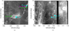 |
Fig. 1. Positions of the spectra (overlaid on M3 spectral reflectance at 1.579 μm) selected to illustrate the spectral differences of compaction and space-weathering in Figs. 3 and 4 from the Reiner Gamma (a) and Dufay Swirls (b). |
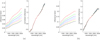 |
Fig. 2. Spectral trend due to soil compaction computed based on the model by Hapke (2008). The darkest line in each plot corresponds to the measured spectrum. The brighter spectra are modeled based on the filling factor of the model by Hapke (2008) with increasing soil compaction. Panel a: mature mare spectrum (average of 1 km2 area at 14.167° E, 21.700° N). Panel b: mature highland spectrum (average of 1 km2 area at 182.400° E, 2.233° N). The filling factor ranges from 0 (bottom curve) to 0.6 (top curve) in steps of 0.1. |
To quantify the similarity of an observed spectral trend to reduced space-weathering vs. soil compaction, we use the compaction-significance spectral index (CSSI), a positive real number defined by a pair of spectra located on a bright and a dark surface, respectively. Small values of CSSI are typical of fresh impact craters, whereas large values indicate a spectral trend inconsistent with reduced space-weathering alone. Accordingly, we also present maps of the CSSI for the examined mare and highland swirls to examine whether the observed on-swirl vs. off-swirl spectral trends can be explained by reduced space-weathering alone.
2.1. Definition of the compaction-significance spectral index
The modulation at 1.579 μm wavelength between a dark off-swirl spectrum (index d) and a brighter on-swirl spectrum (index b) is given by:
 (1)
(1)
the root square deviation between the normalized dark spectrum Sd(λ) and the normalized bright spectrum Sb(λ) by:
![Mathematical equation: $$ \begin{aligned} \mathrm{RSE} = \sqrt{\int \limits _{661\,\mathrm{nm} }^{2577\,\mathrm{nm} } \left[ S_b(\lambda ) - S_d(\lambda )\right]^2 \mathrm{d}\lambda }. \end{aligned} $$](/articles/aa/full_html/2020/07/aa37299-19/aa37299-19-eq2.gif) (2)
(2)
The integral in Eq. (2) covers the wavelength range from 661 nm to 2577 nm corresponding to M3 channels 6 to 75. Larger wavelengths are neglected in order to exclude the 3 μm absorption band, which exhibits systematic differences between on-swirl and off-swirl material. We found the RSE to increase with modulation M1579. For a given M1579, small RSE values were found for the soil compaction trend predicted by the Hapke (2008) model and large values for a spectral trend due to reduced space-weathering. Hence, we defined the compaction-significance spectral index (CSSI) as:
 (3)
(3)
where small values of CSSI indicate similarity to a spectral trend due to reduced space-weathering and large values similarity to the modeled soil compaction trend. Hence, the value of the CSSI provides direct information about the relative importance of reduced space-weathering and soil compaction, given a pair of on-swirl vs. off-swirl spectra.
In the case of pure compaction and in the absence of noise, the model from Hapke (2008) yields a CSSI of ~0.7 that is largely independent of the modulation M1579. Adding noise to the reflectance spectra decreases the CSSI because the RSE value increases. When Gaussian noise with a standard deviation of 0.5% is added to the reflectance spectra, which is a realistic value, the CSSI decreases to ~0.4 for pure compaction.
2.2. The M3 data processing framework
The measured properties of the OH/H2O absorption band highly depend on the method used for thermal emission removal. Due to the commonly known (Bandfield et al. 2015, 2016, 2018; Milliken & Li 2017; Li & Milliken 2016) systematic underestimation of the surface temperature within the M3 level 2 data set on the PDS (Isaacson et al. 2011; Clark et al. 2011), we use the M3 level 1B spectral radiance image data from the PDS1.
As a correction for thermal emission, we apply the technique of Wöhler et al. (2017a,b), which uses the spectral single-scattering albedo to model the reflectance and the emissivity of the surface. The method of Shkuratov et al. (2011), which assumes that the surface is in thermal equilibrium, is then adapted to infer a surface temperature. Since the single-scattering albedo depends on the correct removal of the thermal emission component, Wöhler et al. (2017a,b) used a superposition of a linearly extrapolated reference reflectance spectrum and the thermal emission of a black body to compute an initial temperature value. The spectral reflectance, spectral emissivity, and surface temperature are then refined by applying an iterative update scheme. This procedure is repeated until the change in temperature between two iterations falls below 0.01 K. Notably, this approach simultaneously yields the surface temperature and the wavelength-dependent spectral emissivity of the surface. Another factor influencing the thermal emission component is the small-scale roughness of the surface (Bandfield et al. 2015; Davidsson et al. 2015). Assuming that a rough surface may be described by small facets providing local plane approximations to the surface, the observed thermal emission spectrum corresponds to the superposition of all facets’ thermal emissions. Consequently, the thermal emission component cannot be represented by one single black body emission spectrum or one single temperature value. The wavelength range of the M3 instrument, however, is limited to 3000 nm. Wöhler et al. (2017a) showed that across the limited wavelength range of the M3 instrument the sum of thermal emission spectra can be approximated at high accuracy by a black body spectrum defined by an effective temperature. We adopt the method of Wöhler et al. (2017a) to obtain the temperature difference between the thermal equilibrium based temperature estimation and the effective temperatures for various degrees of surface roughness and incidence angles. Here, we assume a surface roughness of 9° root-mean-square slope (Wöhler et al. 2017a; Grumpe et al. 2019). Wöhler et al. (2017b) showed that the maps of the 3 μm band depth remain qualitatively similar when the assumed surface roughness is increased to the value of 20° proposed by Bandfield et al. (2015, 2018).
Both the estimation of accurate surface temperature values and the reflectance normalization to uniform illumination and observation conditions require a sufficiently well resolved detailed topographic map. As described in detail by Wöhler et al. (2014), we use for this purpose the GLD100 topographic map (Scholten et al. 2012) in combination with the photoclinometry-based approach by Grumpe & Wöhler (2014). We apply the photometric normalization method of Grumpe et al. (2014) which infers the single-scattering albedo of the Hapke model (Hapke 1984, 2002) for each pixel. The normalized spectral reflectance is then obtained by inserting the estimated single-scattering albedo, using a uniform incidence and emission angle of 30° and 0° (Isaacson et al. 2011), respectively, for each channel. The remaining Hapke model parameters are adopted from the first global lunar set of Hapke model parameters by Warell (2004).
3. Results
3.1. Behavior of the 3 μm band depth
For all examined magnetic anomalies (Table 1), 3 μm band depth maps are provided for as many local times of day as possible, where “morning”, “midday” and “afternoon” maps were assembled from M3 data acquired at local times between 07:00–08:00, 10:00–14:00 and 16:00–17:00 hours local time, respectively. The 3 μm band depth is given as the average relative absorption depth across the wavelength range 2.697–2.936 μm (Wöhler et al. 2017b). Maps of the mare swirl Reiner Gamma and the highland swirl near Dufay (the latter not being very prominent at visible and NIR wavelengths but distinguishable at UV wavelengths, see Denevi et al. 2016) are shown in Figs. 5–6 and maps of the other examined swirls in Figs. 7–A.6. To the east of the swirl near Dufay, a bright region is apparent (see also Denevi et al. 2016) which shows up as an area of strongly increased 3 μm band depth (see Wöhler et al. 2019, for details). On the surface around the magnetic anomalies, the 3 μm band depth is weaker at midday than in the morning and afternoon, which is the general behavior in the lunar maria and highlands (Wöhler et al. 2017b). On the swirls, the 3 μm band is typically weaker than in their surroundings and shows only slight variations during the lunar day. All examined swirls except the swirl in Mare Moscoviense (Blewett et al. 2011; Denevi et al. 2016) exhibit a negative anomaly in 3 μm band depth with respect to the surrounding surface (i.e., the 3 μm band is weaker on-swirl than off-swirl). Similar to Li & Garrick-Bethell (2019), our results indicate a weaker 3 μm band inside than outside the magnetic anomalies for the Reiner Gamma and Gerasimovich swirls (for a general description of these swirls see Blewett et al. 2011; Denevi et al. 2016). Our time-of-day-dependent analysis reveals that for Reiner Gamma and the highland swirls near Gerasimovich and Hayford E (the authors are not aware of a previous description of the structure near Hayford E, but its associated magnetic anomaly is apparent in the magnetic flux density maps of Tsunakawa et al. 2015; Denevi et al. 2016), the decrease in 3 μm band depth between morning and midday is much weaker for the swirl than for the surrounding surface. For the swirls in Mare Ingenii and near Dufay only M3 data acquired at local midday are available. The small swirl in Mare Moscoviense (Fig. 7) does not exhibit a 3 μm band depth anomaly but behaves like the surrounding mare surface. Furthermore, another high-albedo pattern corresponds to a unique strongly positive 3 μm band depth anomaly located slightly off the center of the associated magnetic anomaly (i.e., the 3 μm band is stronger on than off the bright structure, see Fig. 6). The special nature of this structure has been subject of a previous study (Wöhler et al. 2019).
3.2. On-swirl vs. off-swirl spectral trends
For a large number of locations on each swirl, we manually defined pairs of points at on-swirl and nearest off-swirl locations, respectively. Similar series of spectra from on-swirl to off-swirl locations were analyzed by Pieters & Noble (2016) and Bhatt et al. (2018). For each pair of points, the CSSI was computed as shown in Figs. 5e, 6d and 7e. For Reiner Gamma, the same was done for various small fresh craters in the surrounding mare region to check if a similar spectral behavior can be observed. Typical on-swirl vs. off-swirl spectral trends are shown in Fig. 3 with the corresponding locations and CSSI values listed in Table 2.
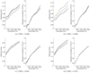 |
Fig. 3. Measured spectral trends from on-swirl to off-swirl locations for spectral pairs representing a spectral trend consistent with reduced space-weathering and increased soil compaction, respectively. Panels a, b: mare swirl Reiner Gamma. Panels c, d: highland swirl near Dufay. The footprint size of the spectra is 700 × 700 m. Each series of spectra was extracted at seven equidistant points on the straight line connecting the on-swirl location with the corresponding off-swirl location. The spectra which are brightest and darkest at 1.579 μm, respectively, were used to compute the compaction-significance spectral index (see Sect. 2). The wavelength range is 0.661 μm to 2.577 μm. |
To further illustrate the difference of the spectral trends due to space-weathering and compaction, we used the model of Hapke (2008) to examine the influence of the filling factor, and we employed the Mie-scattering based technique by Wohlfarth et al. (2019) to model the effects of space-weathering. If the on-swirl and off-swirl spectral difference can be best explained by space-weathering, we expect that we will be able to reproduce the off-swirl spectrum by artificial space-weathering of the on-swirl spectrum relatively precisely. The artificially compacted off-swirl spectrum should then be less similar to the on-swirl spectrum, and the other way round for a spectral difference best explained by compaction. We selected two typical pairs of off-swirl and on-swirl locations at Reiner Gamma, one with a high and another with a low CSSI. The measured on-swirl and off-swirl spectra with their respective space-weathered and compacted spectra are shown in Fig. 4.
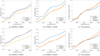 |
Fig. 4. Illustration of the different spectral trends for two on-swirl and off-swirl pairs of spectra from Reiner Gamma. Panels a–c: pair of spectra with a low CSSI, where the space-weathering model provides a better fit. Panels d–e: pair of spectra with a high CSSI, where the soil compaction model provides a better fit. The best-fit spectra for a compacted off-swirl spectrum are shown in panels a and d. On-swirl spectra that have been artificially space-weathered according to Wohlfarth et al. (2019) to obtain a best fit to the measured off-swirl spectrum are shown in panels b and e. The locations of the spectra are displayed in Fig. 1a. The exact locations, best-fit model parameter values and CSSI values are listed in Table 3. The best-fit root mean squared errors (RMSE) are listed in the captions of the individual diagrams. |
We expect the magnetic field to be effective in reducing the space-weathering, but we do not expect it to alter the entire nature of space-weathering. On the Moon, space-weathering is always associated with reddening of the spectral continuum and dampening of the absorption bands due to submicroscopic iron particles being formed (e.g., Hapke 2001; Lucey & Riner 2011). Besides solar wind particles, meteoroid impacts may produce nanophase iron (npFe) particles (e.g., Markley & Kletetschka 2016; Thompson et al. 2017). The npFe particles (< 100 nm diameter) are mainly responsible for the spectral reddening, whereas the larger microphase iron (mpFe) particles (> 100 nm diameter) are mainly responsible for the darkening (Lucey & Riner 2011; Britt & Pieters 1994).
In principle, the space-weathering model by Wohlfarth et al. (2019) used in this work is able to account for very large mpFe particles with radii of up to 115 nm that may compensate for the reddening effect, whereas traditional models (e.g., Hapke 2001) only consider the smaller npFe particles. Transmission electron microscopy measurements conducted by Pieters & Noble (2016), though, have not shown iron particles in mature lunar samples as large as the mpFe particles required by our model to compensate for the reddening effect.
Therefore, we expect the mpFe weight percentage of areas where the CSSI is low, corresponding to a difference mainly in maturity, to be representative for the region around a swirl. When modeling all location pairs at Reiner Gamma with a relatively low CSSI (CSSI < 0.04), also including a few fresh mare craters, we obtained a mean weight percentage of mpFe of 0.17 wt%. This value is consequently used in all our modeled spectra. Not applying this constraint would mean that the mpFe content is variable by a factor of three to four across the mature soil around the swirl (where the magnetic shielding is absent and thus cannot influence the space-weathering), which is not plausible as the intensity and composition of the solar wind are supposed to be uniform outside the magnetic field.
Additionally, it should be noted that the npFe and mpFe weight percentages are only a relative measure for the difference in space-weathering between on-swirl and off-swirl spectra and do not necessarily represent the absolute weight percentage of npFe and mpFe particles in each of the measured spectra. Consequently, pairs with a low CSSI correspond to the highest difference in maturity and, therefore, the actual difference in mpFe for pairs with high CSSI values is probably even lower than the default value used.
The mpFe maps created by Trang & Lucey (2019) with the Lucey & Riner (2011) model using Kaguya Multiband Imager data illustrate that there are only minor differences in mpFe between locations on the swirl and next to it. Their maps furthermore show that the npFe weight percentage is strongly different between on-swirl and off-swirl locations and also varies between the locations of our selected spectral pairs. While the model of Lucey & Riner (2011) and the model of Wohlfarth et al. (2019), which is used in this work, are different, both use npFe und mpFe particles to reproduce the spectral trends observed due to space-weathering. Using the fixed mpFe weight percentage of 0.17 wt% for the complete region and optimizing only for the best-fit npFe weight percentage, we obtained the following results.
Figure 4 shows that the first pair of spectra (Figs. 4a–c) can be best explained by a difference in maturity. Figure 4a indicates that the compacted off-swirl spectrum does not fit the on-swirl spectrum well, but rather the space-weathered on-swirl spectrum fits the off-swirl spectrum as seen in Fig. 4b. The other pair (Figs. 4d–e) corresponds to a high CSSI of about 0.09. This spectral pair can best be modeled with compacting the off-swirl spectrum by increasing the filling factor (see Fig. 4d). The space-weathered on-swirl spectrum cannot accurately describe the mature off-swirl spectrum, because there is no reddening of its continuum slope and its absorption bands are not less pronounced than in the on-swirl spectrum. While this effect could in principle be modeled by adding large amounts of mpFe (about three to four times the default value used), this would require a different process contradicting the common assumptions made about the spectral effects of lunar space-weathering. As can be seen in the normalized spectra (Figs. 4c and f), the compacted on-swirl spectra have the same normalized spectral slope and, therefore, can hardly be distinguished from the corresponding off-swirl spectra in normalized reflectance, see also the modeling result for a pair with a very high CSSI of 0.34 shown in Fig. A.2. A similar spectral trend has been found by Pieters & Noble (2016) for a location on Reiner Gamma. This modeling illustrates that the CSSI is a tradeoff factor between the spectral trends of space-weathering and compaction modeled with the filling factor. Both processes are likely to be present, but either one might be more dominant, depending on the location.
As shown in Fig. 5e, in the central bright “oval” part of the mare swirl Reiner Gamma the CSSI obtains values of ~0.03, comparable to the surrounding small fresh craters. However, in the southwestern part of the central “oval”, the small “flower” structures southwest of it and in the northern part of the “tail,” moderately large values of CSSI in the range 0.1–0.2 and in some places even very large values exceeding 0.2 are found. The central “oval” of Reiner Gamma is strongly shielded by the magnetic field, which reaches a magnetic flux density of 508.2 nT, and, therefore, we assume that here the shielding from the solar wind is the main factor for the explanation of the high albedo. This is consistent with the mainly small values of the CSSI. In the “tail” of Reiner Gamma magnetic shielding is also present, but here the high values of the CSSI suggest that the dominant process leading to increased albedo appears to be a difference in compaction. The magnetic shielding in the “tail” is significantly weaker with a maximum magnetic flux density of up to only 132 nT.
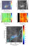 |
Fig. 5. Mare swirl Reiner Gamma. White arrows indicate swirl structures, black pixels denote missing data. Panel a: images from the Lunar Reconnaissance Orbiter Camera Wide Angle Camera (LROC WAC; Robinson et al. 2010) mosaic (Wagner et al. 2015)2 with Kaguya magnetic flux density maps at surface level (Tsunakawa et al. 2015) as overlay. Panel b: M3 reflectance at 1.579 μm. Panels c and d: integrated 3 μm band depth (OHIBD). Panel e: CSSI, overlaid on M3 reflectance at 1.579 μm. |
As an independent verification of the spectral differences between the “oval” and the “tail” of Reiner Gamma, we performed a principal component analysis (PCA; Marsland 2015), similar to Chrbolkova et al. (2019). Figure A.1e shows the mean spectrum of the region. The eigenvectors of the covariance matrix, the so-called principal components, contain information about trends in the data but are usually difficult to interpret in an intuitive way (e.g., Chrbolkova et al. 2019). However, in this special case the first component, describing most of the variance in the data, can be interpreted to contain information about the 1 μm and 2 μm absorption bands (Fig. A.1f). The second component indicates a “bluening” of the spectrum occurring in the transition from mature to immature soils (Fig. A.1g). The score maps of the second and the third principal component show systematic differences between the “oval” and the “tail” (Fig. A.1). In the score map of principal component 2 (Fig. A.1b) the bright “tail” is hardly distinguishable from the surrounding mare surface, confirming that the spectral properties of the “tail” systematically differ from those of the “oval”.
At the Dufay swirl, the CSSI is lowest where the magnetic shielding is strongest (Fig. 6d), similar to Reiner Gamma. No clear trends are apparent at the Moscoviense, Ingenii, Gerasimovich and Hayford E swirls (Figs. A.4d, A.5f and A.6e). Large values of CSSI are observed in small areas of all examined swirls, that is, in the western part of the Dufay highland swirl and the southern part of the bright structure to the east (Fig. 6d), the Mare Ingenii swirl (Fig. A.4d), the central, southern and eastern part of the Gerasimovich swirl (Fig. A.5f), and the central-eastern part of the Hayford E swirl (Fig. A.6e). For the small swirl in Mare Moscoviense, the CSSI is generally lower but also reaches values larger than 0.1 (Fig. 7e). Interestingly, also the rays close to the fresh crater Mandelshtam F southwest of the Dufay swirl exhibit large values of the CSSI (Fig. 6d).
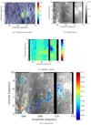 |
Fig. 6. Swirl near Dufay. White arrows indicate swirl structures, black pixels denote missing data. Panel a: LROC WAC mosaic (Wagner et al. 2015) with Kaguya magnetic flux density maps at surface level (Tsunakawa et al. 2015) as overlay. Panel b: M3 reflectance at 1.579 μm. Panel c: 3 μm band depth. Panel d: CSSI, overlaid on M3 reflectance at 1.579 μm. |
4. Discussion
The flux of solar wind protons is modulated by magnetic fields on small to large spatial scales (Kallio et al. 2019; Hemingway & Tikoo 2018). In principle, the occurrence of negative 3 μm band depth anomalies in association with magnetic anomalies for all examined swirls except the Mare Moscoviense swirl is consistent with the common assumption that inside the magnetic anomaly the solar wind proton flux at the surface is lower than outside (e.g., Kramer et al. 2011; Blewett et al. 2011) or prevents their deep penetration into the regolith by reducing their velocity (Farrell et al. 2017), thus reducing the rate of subsequent reactions with surface-bound oxygen.
The Mare Moscoviense swirl, which is associated with a weak maximum magnetic field at surface level of only 11.44 nT (Table 1, Fig. 7a), does not exhibit a 3 μm band depth anomaly. This behavior is consistent with the probable lack of magnetic shielding.
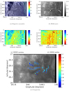 |
Fig. 7. Swirl in Mare Moscoviense. White arrows indicate swirl structures, black pixels denote missing data. Panel a: LROC WAC mosaic (Wagner et al. 2015) with Kaguya magnetic flux density maps at surface level (Tsunakawa et al. 2015) as overlay. Panel b: M3 reflectance at 1.579 μm. Panels c and d: 3 μm band depth (morning, midday). Panel e: CSSI, overlaid on M3 reflectance at 1.579 μm. |
Our observations indicate that outside the magnetic anomalies the difference between the morning or afternoon and the
midday 3 μm band depth values is smaller than about 30%. In contrast, surficial H column densities about ten to one hundred times higher in the morning and afternoon than at midday are predicted by the model of Farrell et al. (2017) for the low-latitude range in which the examined magnetic anomalies are located. This discrepancy might be explained by the presence of a more strongly bound OH/H2O component (e.g., Bandfield et al. 2016; Li & Milliken 2017), which may be quenched in agglutinates (Li & Milliken 2017). This component is not subject to diffusive loss and photolysis. The observed 3 μm band depth then corresponds to an additive combination of the strongly bound component and the weakly bound, time-of-day-dependent component (Li & Milliken 2017; Wöhler et al. 2017b; Grumpe et al. 2019).
The reduced 3 μm band depth at on-swirl vs. off-swirl locations is also detectable at midday. This observation suggests that also the strongly bound OH/H2O component is less abundant inside than outside the magnetic anomalies and is thus dependent on the solar wind flux. Consequently, the strongly bound component is not completely due to hydrated minerals. Rather, it might consist of OH/H2O induced by solar wind protons that underwent diffusion into binding states of sufficiently high energy in the surface mineral that it is not susceptible to diffusive loss and photolysis on time scales comparable to the lunar day. It has been shown that due to the presence of darkening agents, such as ilmenite, the 3 μm absorption band depth is expected to decrease with decreasing albedo (Milliken & Mustard 2007). To explain our observation that the 3 μm band is weaker inside than outside a magnetic anomaly, the abundance of the darkening agent would have to be higher on-swirl than off-swirl. In contrast, to explain the high swirl albedo, the abundance of the darkening agent would have to be lower on-swirl than off-swirl. Hence, variations in the abundance of darkening agents are not able to explain both the albedo and the behavior of the 3 μm band depth. Furthermore, as pointed out by Kramer et al. (2011) there is no plausible process that is able to explain how the darkening agent should have been removed from the on-swirl location. Therefore, we assume that this effect has no significant influence on the estimation of the 3 μm band depth.
On the one hand, the mechanism of magnetic shielding is thus consistent with the observation of reduced space-weathering at the swirls, corresponding to the small CSSI values smaller than 0.05 exhibited by all swirls examined in this study. On the other hand, this mechanism alone cannot explain the observed peculiar spectral signatures showing nearly no variation in normalized reflectance between on-swirl and off-swirl surfaces, as indicated by large CSSI values in the range 0.1–0.2 and even higher in some parts of all examined swirls. Of course, a possible explanation for compacted soil is that magnetic shielding may also be able to prevent the surface from becoming as porous as the surrounding soil. Highly porous and fine-grained regolith often referred to as “fairy castle” (Hapke & van Horn 1963) is created by gardening of the regolith by micrometeorites and solar radiation (e.g., Hapke & van Horn 1963). This would, however, suggest that the magnetic field shields the surface also from micrometeorite impact, which is generally assumed to be not the case (e.g., Chrbolkova et al. 2019), or that the high porosity of mature regolith is mainly caused by charged particles of the solar wind rather than by micrometeorites, which would be physically unintuitive.
Consequently, the peculiar spectral signatures indicating compacted soil provide evidence for the occurrence of an additional physical process beyond magnetic shielding. As a possible external mechanism, the interaction between the regolith and cometary gas has been suggested (e.g., Gold & Soter 1976; Shevchenko 1993; Pinet et al. 2000), which might be similar to the effect of a landing rocket jet (e.g., Shevchenko 1993). This mechanism can explain the observed on-swirl vs. off-swirl spectral trends in the following ways:
It has been proposed that the magnetic field is also relevant to explaining the origin of swirls. The separation between magnetic and non-magnetic grains has been proposed to be an explanation for the spectral signatures on and around swirls (Pieters & Garrick-Bethell 2015; Pieters 2018). Magnetic materials are darker than non-magnetic materials (Adams & McCord 1973), so that a removal of the magnetic components from the swirl would lead to a difference in albedo. Furthermore, the normalized spectral slope of magnetic samples is larger than that of non-magnetic samples, resulting in a relatively low CSSI of 0.044 (Fig. A.3b). The pair of spectra for a dark lane and an on-swirl spectrum from Pieters (2018) shown in Figs. A.3c and d corresponds to a CSSI of 0.108, a similarity that suggests a difference in compaction rather than a difference in maturity. The spectral difference of non-magnetic and magnetic grains is similar to the space-weathering trend described in Sect. 3.2. The process of magnetic separation is thus able to explain spectral trends with low CSSI values, but not the occurrence of spectral trends associated with large CSSI values attributed to soil compaction in Sect. 3.2.
The spectral signatures of reduced space-weathering observed for all examined swirls can be explained by the removal of an uppermost very thin, strongly mature regolith layer by the cometary gas, where the newly exposed regolith will undergo reduced space-weathering due to the presence of localized magnetic shielding. A similar process is described by Wu & Hapke (2018) in their analysis of reflectance spectra of the regolith near the Chang’e-3 lander affected by the landing rocket jet, which were acquired by the VNIS instrument on-board the Yutu rover. Their series of spectra exhibit a clear space-weathering trend. This will preferentially happen when the gas moves approximately parallel to the surface. Wu & Hapke (2018) point out that the gas jet of the landing rocket removed only a very thin layer of regolith and did not change the surface roughness. This would support the finding of Glotch et al. (2015) that the surface roughness is not altered at swirls. Wu & Hapke (2018) also assumed that only the finest regolith fraction might be removed by the gas jet. However, a difference between on-swirl and off-swirl material in average grain size alone would not be able to explain the difference in albedo. Immature soils are known to be more coarsely grained than mature soils (e.g., Dollfus 1999), and coarsely grained regolith always has a lower albedo than finely-grained regolith of the same composition (e.g., Kramer et al. 2011), so that the coarse grain size supposedly associated with the immature on-swirl locations cannot explain their high albedo. Garrick-Bethell et al. (2011) suggested the opposite effect as an explanation for the albedo difference, meaning that, in their model, the finely grained regolith fraction is transported to the swirl locations by electric fields generated by separation of charged solar wind particles due to the local magnetic field. This requires a systematic sorting of the grains over long periods of time as a consequence of periodically recurrent differential grain motion during lifting of the regolith at sunrise and sunset. Furthermore, to explain the spectral behavior of swirls that deviates from reduced space-weathering, their model requires an increased component of highland material at on-swirl relative to off-swirl locations, whose origin is not obvious.
Depending on its direction of motion, the cometary gas may also lead to compaction of the regolith. To explain the increase in swirl albedo (which is at most a factor of 1.5 relative to a “normal” surface) by regolith compaction alone, that is, without changing the maturity, the Hapke (2008) model indicates that the filling factor of the regolith would have to be increased from its typical value of 0.3 (Hapke 2008) to about 0.5–0.6 (Fig. 2a). The uppermost centimeters of the regolith determine its thermal properties (Vasavada et al. 1999). Hence, compression of a very thin regolith layer of only a few grains thickness would explain the observed reflectance properties due to the limited penetration depth of NIR photons of at most several microns, while in agreement with the findings by Glotch et al. (2015) this compression would not change the bulk thermal properties of the regolith. It is also consistent with the finding by Neish et al. (2011) that swirls are very thin.
Here, the mechanism of complete or partial magnetic shielding continues to be of essential importance to explain the current appearance of the swirl patterns, because it maintains the observed high-albedo structures and negative 3 μm band depth anomalies over long periods. The existence of the Mare Moscoviense swirl, where magnetic shielding is supposedly absent or much weaker than for the other examined swirls, may be explained by interaction with cometary gas that happened so recently that no significant space-weathering effects could occur since then.
The occurrence of large CSSI values (> 0.2) on the ejecta blanket of the fresh ~15 km diameter crater Mandelshtam F at distances from the center of up to two to three crater diameters (Fig. 6) can be explained in the way that in the vicinity of the crater the bright structures are due to localized strong compaction of the immature continuous ejecta deposits near the crater. At larger distances from the crater, the rays oriented in the north-eastern direction show a spectral trend that is more similar to reduced space-weathering (CSSI ≲ 0.05) compared to the rays oriented in northern direction (CSSI ≈ 0.1). This behavior may be due to an asymmetric distribution of the crater ejecta, where a broad streak of bright ejecta material extends from the crater to the north. Assuming that this immature material is overlaid by narrow bright filaments of similarly immature but compacted material would explain the large CSSI values inferred for the northern ray. In contrast, the northwestern rays were deposited directly on relatively dark and thus mature highland material, so that the inferred small CSSI values reflect the difference in maturity between the northeastern rays and the surrounding surface.
Shevchenko (1993) estimated the age of Reiner gamma formation to be about 40 million years and stated that within the last 40 million years about 40 swirl-forming events could have occurred. This estimate, however, did not consider the magnetic shielding of the surface, which is supposed to extend the lifetime of the swirl structures substantially. The size of a comet responsible for the formation of Reiner gamma is estimated to be three to four km by Pinet et al. (2000). Hydrodynamic modeling of the origin of swirls due to interaction between cometary coma and the lunar surface shows that the impact of 1 km large comets can explain the properties of the observed swirls (Bruck Syal & Schultz 2015). In that work, the frequency of 1 km large comet impacts with the Moon was estimated to be one impact per 29 million years. For more accurate estimates of the size of swirl-forming comets, one needs to better know the properties of the lunar regolith. The estimated dynamic pressure of the gas for Apollo exhaust events is about 6890 N m−2 and it was large enough to decrease the porosity and to change reflectance properties of the regolith near the landing site (Hinners & El-Baz 1972). Additional studies of the influence of the interaction of cometary gas with the surface on porosity and reflectance properties of the lunar surface are needed. To further quantify and validate the presented model, it would be necessary to know the age of the swirls and how long magnetic shielding can preserve the albedo markings. If these parameters were known, they could be compared to the influx of comets and how frequently such interaction events occur.
5. Conclusion
Our results show that magnetic shielding alone is not able to explain all spectral trends observed at swirls. The time-of-day-dependent variations of the 3 μm integrated band depth indicating the OH/H2O content in the uppermost layer of the regolith are less pronounced at most on-swirl locations compared to the surrounding areas. This shows that the solar wind influx at magnetically shielded locations is subdued, which might have led to reduced space-weathering. Other swirl locations, however, that show a similarly high albedo do not appear to be immature. To quantify these differences, the compaction-significance spectral index (CSSI) as a tradeoff factor between reduced space-weathering and regolith compaction was defined. Many swirl locations were found which do not show spectral differences between on-swirl and off-swirl locations that can be explained by reduced space-weathering, but rather by regolith compaction. A more compact soil appears brighter, but the normalized spectrum does not change its spectral slope and the absorption bands are not subdued. These areas showing high CSSI values, supports the hypothesis that swirl formation is due to the interaction of the regolith with external influences, such as cometary gas. Another possible explanation of the high CSSI values is that magnetic shielding also prevents the surface from becoming as porous as those areas of the surface that are exposed to the space environment.
Acknowledgments
C. W. and A. G. were funded by the Deutsche Forschungsgemeinschaft (DFG, German Research Foundation), project no. 277133575. A. A. B. was partially supported by TU Dortmund University. A. A. B. and V. V. S. were partially supported by the Russian Science Foundation, grant no. 20-12-00105.
References
- Adams, J. B., & McCord, T. B. 1973, 4th Lunar Planet. Sci. Conf. Proc., 164 [Google Scholar]
- Bamford, R. A., Alves, E. P., Cruz, F., et al. 2016, ApJ, 830, 146 [NASA ADS] [CrossRef] [Google Scholar]
- Bandfield, J. L., Hayne, P. O., Williams, J.-P., et al. 2015, Icarus, 248, 357 [NASA ADS] [CrossRef] [Google Scholar]
- Bandfield, J. L., Edwards, C. S., Poston, M. J., et al. 2016, Lunar H2O/OH-Distributions: Revised Infrared Spectra from Improved Thermal Corrections, LPSC XXXXVII, Abstract, 1594 [Google Scholar]
- Bandfield, J. L., Poston, M. J., Klima, R. L., et al. 2018, Nat. Geosci., 11, 173 [NASA ADS] [CrossRef] [Google Scholar]
- Bhardwaj, A., Dhanya, M. B., Alok, A., et al. 2015, Geosci. Lett., 2, 10 [NASA ADS] [CrossRef] [Google Scholar]
- Bhatt, M., Wöhler, C., Srivastava, N., et al. 2018, Regolith Alteration Processes at Reiner Gamma Shed Light on the Formation of Lunar Swirls, LPSC XLIX, abstract, 1765 [Google Scholar]
- Blewett, D. T., Denevi, B. W., Robinson, M. S., et al. 2010, Icarus, 209, 239 [NASA ADS] [CrossRef] [Google Scholar]
- Blewett, D. T., Coman, E. I., Ray Hawke, B., et al. 2011, J. Geophys. Res., 116, E02002 [NASA ADS] [Google Scholar]
- Britt, D. T., & Pieters, C. M. 1994, Geochim. Cosmochimica Acta, 58, 3905 [Google Scholar]
- Bruck Syal, M., & Schultz, P. H. 2015, Icarus, 257, 194 [CrossRef] [Google Scholar]
- Chrbolkova, K., Kohout, T., & Durech, J. 2019, Icarus, 333, 516 [NASA ADS] [CrossRef] [Google Scholar]
- Clark, R. N., Pieters, C. M., Green, R. O., Boardman, J. W., & Petro, N. E. 2011, J. Geophys. Res., 116, E00G16 [CrossRef] [Google Scholar]
- Coleman, P. J., Schubert, G., Russell, C. T., et al. 1972, The Moon, 4, 419 [NASA ADS] [CrossRef] [Google Scholar]
- Davidsson, B. J. R., Rickman, H., Bandfield, J. L., et al. 2015, Icarus, 252, 1 [NASA ADS] [CrossRef] [Google Scholar]
- Deca, J., Hemingway, D. J., Divin, A., et al. 2020, J. Geophys. Res. Planets, 125, e2019JE006219 [CrossRef] [Google Scholar]
- Denevi, B., Robinson, M. S., Boyd, A. K., et al. 2016, Icarus, 273, 53 [CrossRef] [Google Scholar]
- Dollfus, A. 1999, Icarus, 140, 313 [NASA ADS] [CrossRef] [Google Scholar]
- Dyal, P., Parkin, C. W., Sonett, C. P., et al. 1970, Science, 169, 762 [NASA ADS] [CrossRef] [Google Scholar]
- Farrell, W. M., Hurley, D. M., Zimmerman, M. I., et al. 2015, Icarus, 255, 116 [CrossRef] [Google Scholar]
- Farrell, W. M., Hurley, D. M., Esposito, V. J., et al. 2017, J. Geophys. Res., 122, 269 [NASA ADS] [CrossRef] [Google Scholar]
- Garrick-Bethell, I., Head, J. W., & Pieters, C. M. 2011, Icarus, 212, 480 [NASA ADS] [CrossRef] [Google Scholar]
- Gold, T., & Soter, S. 1976, Planet. Space Sci., 24, 45 [NASA ADS] [CrossRef] [Google Scholar]
- Grumpe, A., & Wöhler, C. 2014, ISPRS J. Photogramm. Remote Sens., 94, 37 [NASA ADS] [CrossRef] [Google Scholar]
- Grumpe, A., Belkhir, F., & Wöhler, C. 2014, Adv. Space Res., 53, 1735 [NASA ADS] [CrossRef] [Google Scholar]
- Grumpe, A., Wöhler, C., Berezhnoy, A. A., & Shevchenko, V. V. 2019, Icarus, 321, 486 [NASA ADS] [CrossRef] [Google Scholar]
- Glotch, T. D., Bandfield, J. L., Lucey, P. G., et al. 2015, Nat. Comm., 6, 6189 [NASA ADS] [CrossRef] [Google Scholar]
- Hapke, B. 1984, Icarus, 59, 41 [NASA ADS] [CrossRef] [Google Scholar]
- Hapke, B. 2001, J. Geophys. Res., 106, 10039 [NASA ADS] [CrossRef] [Google Scholar]
- Hapke, B. 2002, Icarus, 157, 523 [NASA ADS] [CrossRef] [Google Scholar]
- Hapke, B. 2008, Icarus, 195, 918 [NASA ADS] [CrossRef] [Google Scholar]
- Hapke, B., & van Horn, H. 1963, J. Geophys. Res., 68, 4545 [NASA ADS] [CrossRef] [Google Scholar]
- Hemingway, D. J., & Tikoo, S. M. 2018, J. Geophys. Res., 123, 2223 [NASA ADS] [CrossRef] [Google Scholar]
- Hendrix, A. R., Retherford, K. D., Randall Gladstone, G., et al. 2012, J. Geophys. Res. (Planets), 117, E12001 [NASA ADS] [CrossRef] [Google Scholar]
- Hinners, N. W., & El-Baz, F. 1972, Surface disturbance at the Apollo 15 landing site, in Apollo 15 Preliminary Science Report (Washington, D.C.: NASA), 25.50 [Google Scholar]
- Hood, L. L. 1995, Earth Moon Planets, 67, 131 [Google Scholar]
- Hood, L. L. 2010, Icarus, 211, 1109 [Google Scholar]
- Hood, L. L., & Schubert, G. 1980, Science, 208, 49 [NASA ADS] [CrossRef] [Google Scholar]
- Hood, L. L., & Williams, C. R. 1989, The Lunar Swirls – Distribution and Possible Origins, LPSC XIX, 99 [Google Scholar]
- Isaacson, P., Besse, S., Petro, N., et al. 2011, in M3 Overview and Working with M3 data. Technical Report [Google Scholar]
- JAXA 2009, KAGUYA (SELENE) Product Format Description -Lunar Magnetometer (LMAG) [Google Scholar]
- Kallio, E., Dyadechkin, S., Wurz, P., & Khodachenko, M. 2019, Planet. Space Sci., 166, 9 [NASA ADS] [CrossRef] [Google Scholar]
- Kramer, G., Besse, S., Dhingra, D., et al. 2011, J. Geophys. Res., 116, E00G18 [Google Scholar]
- Li, S., & Garrick-Bethell, I. 2019, Geophys. Res. Lett., 46, 14318 [NASA ADS] [CrossRef] [Google Scholar]
- Li, S., & Milliken, R. E. 2016, J. Geophys. Res. Planets, 121, 2081 [NASA ADS] [CrossRef] [Google Scholar]
- Li, S., & Milliken, R. E. 2017, Sci. Adv., 3, e1701471 [Google Scholar]
- Lucey, P. G., & Riner, M. A. 2011, Icarus, 212, 451 [NASA ADS] [CrossRef] [Google Scholar]
- Marsland, S. 2015, Machine Learning: An Algorithmic Introduction, 2nd edn. (New Jersey, USA: CRC Press) [Google Scholar]
- Markley, M., & Kletetschka, G. 2016, Icarus, 268, 204 [NASA ADS] [CrossRef] [Google Scholar]
- Milliken, R., & Li, S. 2017, Nat. Geosci., 10, 561 [NASA ADS] [CrossRef] [Google Scholar]
- Milliken, R. E., & Mustard, J. F. 2007, Icarus, 189, 550 [NASA ADS] [CrossRef] [Google Scholar]
- Neish, C. D., Blewett, D. T., Bussey, D. B. J., et al. 2011, Icarus, 215, 186 [CrossRef] [Google Scholar]
- Pieters, C. M. 2018, What Lunar Swirls Represent (.. Probably). 6th European Lunar Symposium (Toulouse, France) [Google Scholar]
- Pieters, C. M., & Garrick-Bethell, I. 2015. Hydration Variations at Lunar Swirls, LPSC XLVI, Abstract, 2120 [Google Scholar]
- Pieters, C. M., & Noble, S. K. 2016, J. Geophys. Res. Planets, 121, 1865 [CrossRef] [Google Scholar]
- Pieters, C. M., Fischer, E. M., Rode, O., & Basu, A. 1993, J. Geophys. Res., 98, 20817 [Google Scholar]
- Pieters, C. M., Boardman, J., Buratti, B., et al. 2009a, Curr. Sci., 96, 500 [Google Scholar]
- Pieters, C. M., Goswami, J. N., Clark, R. N., et al. 2009b, Science, 326, 568 [NASA ADS] [CrossRef] [Google Scholar]
- Pinet, P., Shevchenko, V. V., Chevrel, S. D., et al. 2000, J. Geophys. Res., 105, 9457 [NASA ADS] [CrossRef] [Google Scholar]
- Richmond, N. C., & Hood, L. L. 2008, J. Geophys. Res., 113, E02010 [NASA ADS] [Google Scholar]
- Robinson, M. S., Brylow, S. M., Humm, D., et al. 2010, Space Sci. Rev., 150, 81 [CrossRef] [Google Scholar]
- Scholten, F., Oberst, J., Matz, K.-D., et al. 2012, J. Geophys. Res., 117, E00H17 [CrossRef] [Google Scholar]
- Schultz, P. H., & Srnka, L. J. 1980. Nature, 284, 22 [CrossRef] [Google Scholar]
- Shevchenko, V. V. 1993, Astron. Rep., 37, 314 [NASA ADS] [Google Scholar]
- Shkuratov, Y. G., Kaydasha, V., Korokhin, V., et al. 2011, Planet. Space Sci., 59, 1326 [NASA ADS] [CrossRef] [Google Scholar]
- Starukhina, L. 2001, J. Geophys. Res., 106, 14701 [NASA ADS] [CrossRef] [Google Scholar]
- Sunshine, J., Farnham, T. L., Feaga, L. M., et al. 2009, Science, 326, 565 [NASA ADS] [CrossRef] [Google Scholar]
- Takahashi, F., Shimizu, H., Matsushima, M., et al. 2009, Earth Planets Space, 61, 1269 [NASA ADS] [CrossRef] [Google Scholar]
- Thompson, M. S., Zega, Th. J., & Howe, J. Y. 2017, Meteoritics Planet. Sci., 52, 413 [CrossRef] [Google Scholar]
- Trang, D., & Lucey, P. G. 2019, Icarus, 321, 307 [CrossRef] [Google Scholar]
- Tsunakawa, H., Takahashi, F., Shimizu, H., et al. 2015, J. Geophys. Res. Planets, 120, 1160 [NASA ADS] [CrossRef] [Google Scholar]
- Vasavada, A. R., Paige, D. A., & Wood, S. E. 1999, Icarus, 141, 179 [NASA ADS] [CrossRef] [Google Scholar]
- Vorburger, A., Wurz, P., Barabash, S., et al. 2012, J. Geophys. Res., 117, A07208 [NASA ADS] [Google Scholar]
- Wagner, R. V., Speyerer, E. J., & Robinson, M. S. LROC Team 2015, New Mosaicked Data Products from the LROC Team. Paper presented at the 46th Lunar and Planetary Science Conference (Houston, TX: Lunar and Planetary Institute) [Google Scholar]
- Warell, J. 2004, Icarus, 167, 271 [NASA ADS] [CrossRef] [Google Scholar]
- Weiss, B. P., & Tikoo, S. M. 2014, Science, 346, 1246753 [NASA ADS] [CrossRef] [Google Scholar]
- Wieser, M., Barabash, S., Futaana, Y., et al. 2010, Geophys. Res. Lett., 37, L05103 [Google Scholar]
- Wohlfarth, K., Wöhler, C., & Grumpe, A. 2019, AJ, 158, 80 [NASA ADS] [CrossRef] [Google Scholar]
- Wöhler, C., Grumpe, A., Berezhnoy, A., Bhatt, M. U., & Mall, U. 2014, Icarus, 235, 86 [NASA ADS] [CrossRef] [Google Scholar]
- Wöhler, C., Grumpe, A., Berezhnoy, A. A., et al. 2017a, Icarus, 285, 118 [NASA ADS] [CrossRef] [Google Scholar]
- Wöhler, C., Grumpe, A., Berezhnoy, A. A., & Shevchenko, V. V. 2017b, Sci. Adv., 3, e1701286 [NASA ADS] [CrossRef] [Google Scholar]
- Wöhler, C., Grumpe, A., Bhatt, M., et al. 2019, A&A, 630, L7 [CrossRef] [EDP Sciences] [Google Scholar]
- Wu, Y., & Hapke, B. 2018, Earth Planet. Sci. Lett, 484, 145 [CrossRef] [Google Scholar]
Appendix A: Additional figures
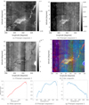 |
Fig. A.1. Maps of the scores of the first three principal components for the Reiner Gamma region. |
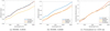 |
Fig. A.2. Spectral pair with a high CSSI of 0.34. The compacted off-swirl spectrum with a filling factor of 0.144 can almost perfectly describe and recreate the on-swirl spectrum. The space weathered on-swirl spectrum with a respective npFe 1.217 wt % and mpFe 0.17 wt% does not recreate the off-swirl spectrum accurately. The position of the spectral pair is marked in Fig. 1. The on-swirl location is: 10.198 ° N, 304.152 ° E and the off-swirl location is: 10.302° N, 303.945° E. The root mean squared errors (RMSE) of the modeled with respect to the measured spectra are listed in the corresponding captions. |
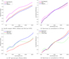 |
Fig. A.3. Comparison of spectral trends described by Pieters (2018, see Fig. 2 therein). The magnetic separates in panel a are taken from RELAB database3, with Sample-IDs LS-JBA-180-M, LS-JBA-180-N and LS-JBA-180-P for magnetic, non-magnetic and bulk samples, respectively. These laboratory spectra were originally acquired by Adams & McCord (1973) and reproduced in Fig. 2B of Pieters (2018). The CSSI for the spectra of magnetic vs. non-magnetic material corresponds to 0.044. The bright swirl, dark lane and fresh crater spectra were derived from M3 data by Pieters (2018), we extracted the spectra shown in panel c manually from Fig. 2A of Pieters (2018). The CSSI value for the spectral pair of bright swirl and dark lane corresponds to 0.108. |
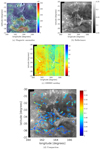 |
Fig. A.4. Swirl in Mare Ingenii. White arrows indicate swirl structures, black pixels denote missing data. Panel a: LROC WAC mosaic (Wagner et al. 2015) with Kaguya magnetic flux density maps at surface level (Tsunakawa et al. 2015) as overlay. Panel b: M3 reflectance at 1.579 μm. Panel c: 3 μm band depth. Panel d: CSSI, overlaid on M3 reflectance at 1.579 μm. |
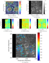 |
Fig. A.5. Swirl near Gerasimovich. White arrows indicate swirl structures, black pixels denote missing data. Panel a: LROC WAC mosaic (Wagner et al. 2015) with Kaguya magnetic flux density maps at surface level (Tsunakawa et al. 2015) as overlay. Panel b: M3 reflectance at 1.579 μm. Panels c–e: 3 μm band depth. (morning, midday afternoon); panel f: CSSI, overlaid on M3 reflectance at 1.579 μm. |
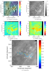 |
Fig. A.6. Swirl near Hayford E. White arrows indicate swirl structures, black pixels denote missing data. Panel a: LROC WAC mosaic (Wagner et al. 2015) with Kaguya magnetic flux density maps at surface level (Tsunakawa et al. 2015) as overlay. Panel b: M3 reflectance at 1.579 μm. Panel c: 3 μm band depth at lunar morning and panel d: at lunar midday. Panel e: CSSI, overlaid on M3 reflectance at 1.579 μm. |
All Tables
Locations and values of maximum modeled magnetic flux density at the surface, extracted from the data set of Tsunakawa et al. (2015).
All Figures
|
Fig. 1. Positions of the spectra (overlaid on M3 spectral reflectance at 1.579 μm) selected to illustrate the spectral differences of compaction and space-weathering in Figs. 3 and 4 from the Reiner Gamma (a) and Dufay Swirls (b). |
| In the text | |
|
Fig. 2. Spectral trend due to soil compaction computed based on the model by Hapke (2008). The darkest line in each plot corresponds to the measured spectrum. The brighter spectra are modeled based on the filling factor of the model by Hapke (2008) with increasing soil compaction. Panel a: mature mare spectrum (average of 1 km2 area at 14.167° E, 21.700° N). Panel b: mature highland spectrum (average of 1 km2 area at 182.400° E, 2.233° N). The filling factor ranges from 0 (bottom curve) to 0.6 (top curve) in steps of 0.1. |
| In the text | |
|
Fig. 3. Measured spectral trends from on-swirl to off-swirl locations for spectral pairs representing a spectral trend consistent with reduced space-weathering and increased soil compaction, respectively. Panels a, b: mare swirl Reiner Gamma. Panels c, d: highland swirl near Dufay. The footprint size of the spectra is 700 × 700 m. Each series of spectra was extracted at seven equidistant points on the straight line connecting the on-swirl location with the corresponding off-swirl location. The spectra which are brightest and darkest at 1.579 μm, respectively, were used to compute the compaction-significance spectral index (see Sect. 2). The wavelength range is 0.661 μm to 2.577 μm. |
| In the text | |
|
Fig. 4. Illustration of the different spectral trends for two on-swirl and off-swirl pairs of spectra from Reiner Gamma. Panels a–c: pair of spectra with a low CSSI, where the space-weathering model provides a better fit. Panels d–e: pair of spectra with a high CSSI, where the soil compaction model provides a better fit. The best-fit spectra for a compacted off-swirl spectrum are shown in panels a and d. On-swirl spectra that have been artificially space-weathered according to Wohlfarth et al. (2019) to obtain a best fit to the measured off-swirl spectrum are shown in panels b and e. The locations of the spectra are displayed in Fig. 1a. The exact locations, best-fit model parameter values and CSSI values are listed in Table 3. The best-fit root mean squared errors (RMSE) are listed in the captions of the individual diagrams. |
| In the text | |
|
Fig. 5. Mare swirl Reiner Gamma. White arrows indicate swirl structures, black pixels denote missing data. Panel a: images from the Lunar Reconnaissance Orbiter Camera Wide Angle Camera (LROC WAC; Robinson et al. 2010) mosaic (Wagner et al. 2015)2 with Kaguya magnetic flux density maps at surface level (Tsunakawa et al. 2015) as overlay. Panel b: M3 reflectance at 1.579 μm. Panels c and d: integrated 3 μm band depth (OHIBD). Panel e: CSSI, overlaid on M3 reflectance at 1.579 μm. |
| In the text | |
|
Fig. 6. Swirl near Dufay. White arrows indicate swirl structures, black pixels denote missing data. Panel a: LROC WAC mosaic (Wagner et al. 2015) with Kaguya magnetic flux density maps at surface level (Tsunakawa et al. 2015) as overlay. Panel b: M3 reflectance at 1.579 μm. Panel c: 3 μm band depth. Panel d: CSSI, overlaid on M3 reflectance at 1.579 μm. |
| In the text | |
|
Fig. 7. Swirl in Mare Moscoviense. White arrows indicate swirl structures, black pixels denote missing data. Panel a: LROC WAC mosaic (Wagner et al. 2015) with Kaguya magnetic flux density maps at surface level (Tsunakawa et al. 2015) as overlay. Panel b: M3 reflectance at 1.579 μm. Panels c and d: 3 μm band depth (morning, midday). Panel e: CSSI, overlaid on M3 reflectance at 1.579 μm. |
| In the text | |
|
Fig. A.1. Maps of the scores of the first three principal components for the Reiner Gamma region. |
| In the text | |
|
Fig. A.2. Spectral pair with a high CSSI of 0.34. The compacted off-swirl spectrum with a filling factor of 0.144 can almost perfectly describe and recreate the on-swirl spectrum. The space weathered on-swirl spectrum with a respective npFe 1.217 wt % and mpFe 0.17 wt% does not recreate the off-swirl spectrum accurately. The position of the spectral pair is marked in Fig. 1. The on-swirl location is: 10.198 ° N, 304.152 ° E and the off-swirl location is: 10.302° N, 303.945° E. The root mean squared errors (RMSE) of the modeled with respect to the measured spectra are listed in the corresponding captions. |
| In the text | |
|
Fig. A.3. Comparison of spectral trends described by Pieters (2018, see Fig. 2 therein). The magnetic separates in panel a are taken from RELAB database3, with Sample-IDs LS-JBA-180-M, LS-JBA-180-N and LS-JBA-180-P for magnetic, non-magnetic and bulk samples, respectively. These laboratory spectra were originally acquired by Adams & McCord (1973) and reproduced in Fig. 2B of Pieters (2018). The CSSI for the spectra of magnetic vs. non-magnetic material corresponds to 0.044. The bright swirl, dark lane and fresh crater spectra were derived from M3 data by Pieters (2018), we extracted the spectra shown in panel c manually from Fig. 2A of Pieters (2018). The CSSI value for the spectral pair of bright swirl and dark lane corresponds to 0.108. |
| In the text | |
|
Fig. A.4. Swirl in Mare Ingenii. White arrows indicate swirl structures, black pixels denote missing data. Panel a: LROC WAC mosaic (Wagner et al. 2015) with Kaguya magnetic flux density maps at surface level (Tsunakawa et al. 2015) as overlay. Panel b: M3 reflectance at 1.579 μm. Panel c: 3 μm band depth. Panel d: CSSI, overlaid on M3 reflectance at 1.579 μm. |
| In the text | |
|
Fig. A.5. Swirl near Gerasimovich. White arrows indicate swirl structures, black pixels denote missing data. Panel a: LROC WAC mosaic (Wagner et al. 2015) with Kaguya magnetic flux density maps at surface level (Tsunakawa et al. 2015) as overlay. Panel b: M3 reflectance at 1.579 μm. Panels c–e: 3 μm band depth. (morning, midday afternoon); panel f: CSSI, overlaid on M3 reflectance at 1.579 μm. |
| In the text | |
|
Fig. A.6. Swirl near Hayford E. White arrows indicate swirl structures, black pixels denote missing data. Panel a: LROC WAC mosaic (Wagner et al. 2015) with Kaguya magnetic flux density maps at surface level (Tsunakawa et al. 2015) as overlay. Panel b: M3 reflectance at 1.579 μm. Panel c: 3 μm band depth at lunar morning and panel d: at lunar midday. Panel e: CSSI, overlaid on M3 reflectance at 1.579 μm. |
| In the text | |
Current usage metrics show cumulative count of Article Views (full-text article views including HTML views, PDF and ePub downloads, according to the available data) and Abstracts Views on Vision4Press platform.
Data correspond to usage on the plateform after 2015. The current usage metrics is available 48-96 hours after online publication and is updated daily on week days.
Initial download of the metrics may take a while.