| Issue |
A&A
Volume 674, June 2023
|
|
|---|---|---|
| Article Number | A226 | |
| Number of page(s) | 21 | |
| Section | Planets and planetary systems | |
| DOI | https://doi.org/10.1051/0004-6361/202346098 | |
| Published online | 27 June 2023 | |
Comparative photometric analysis of the Reiner Gamma swirl and Chang’e 5 landing site
1
Image Analysis Group, TU Dortmund University
Otto-Hahn-Straße 4,
Dortmund, Germany
e-mail: This email address is being protected from spambots. You need JavaScript enabled to view it.
2
Shandong Key Laboratory of Optical Astronomy and Solar-Terrestrial Environment, School of Space Science and Physics, Institute of Space Sciences, Shandong University,
Weihai,
Shandong,
264209, PR China
3
Physical Research Laboratory, University Area,
Ahmedabad, Gujarat
380009, India
Received:
7
February
2023
Accepted:
3
May
2023
Abstract
Context. Lunar swirls are bright albedo features only found on the Moon that are still not entirely understood. It is commonly accepted that reduced space weathering plays a role in explaining the origins of lunar swirls because the local magnetic fields that are typically associated with these albedo anomalies are effective in reducing the solar wind influx. However, additional processes are required to fully explain the spectral, photometric, and polarimetric properties of the swirls.
Aims. In this study, we compare the photometric properties of the Chang’e-5 landing site to those of the Reiner Gamma swirl. Because the physical effects of a landing rocket jet on the lunar regolith are relatively well known, these observations can provide important insights into the physical properties of lunar swirls.
Methods. We determined the single scattering albedo, opposition effect strength, and surface roughness of the Reiner Gamma swirl and the Chang’e-5 landing site with their respective statistical uncertainties based on the Hapke model and Bayesian inference sampling.
Results. The Chang’e-5 landing site and the Reiner Gamma swirl exhibit similar photometric properties, in particular: an increased albedo and a reduced opposition effect strength. Additionally, the landing site is about 20% less rough compared to the surrounding area.
Conclusions. These findings suggest that the swirl surface is less porous compared to the surrounding surface, similarly to a landing site where the top layer of the regolith has been blown away effectively so that the compactness was increased. We conclude that external mechanisms that are able to compress the uppermost regolith layer are involved in lunar swirl formation, such as interactions with the gaseous hull of a passing comet.
Key words: Moon / radiative transfer / scattering / techniques: photometric / methods: statistical
© The Authors 2023
 Open Access article, published by EDP Sciences, under the terms of the Creative Commons Attribution License (https://creativecommons.org/licenses/by/4.0), which permits unrestricted use, distribution, and reproduction in any medium, provided the original work is properly cited.
This article is published in open access under the Subscribe to Open model. This email address is being protected from spambots. You need JavaScript enabled to view it. to support open access publication.
1 Introduction
One of the biggest unsolved mysteries related to our nearest neighbor are lunar swirls. These swirls are characterized by a high-albedo pattern of complex shape and almost all swirls are located at a magnetic anomaly (e.g., Hood & Schubert 1980; Hood & Williams 1989; Tsunakawa et al. 2015). Furthermore, swirls have been found to show a reduced surficial OH/H2O content (Kramer et al. 2011; Hendrix et al. 2016; Li & Garrick-Bethell 2019; Hess et al. 2020a) and the spectral properties appear to be less mature than the surrounding terrain (Glotch et al. 2015; Hendrix et al. 2016; Trang & Lucey 2019; Blewett et al. 2021; Hess et al. 2020a). Previously, it was assumed that there is no correlation between topography and the albedo patterns (Kramer et al. 2011; Denevi et al. 2016), but more recent works have suggested that swirls are marginally lower than the surrounding terrain (Domingue et al. 2022). The photometry of swirls has also been observed to be anomalous. Kreslavsky & Shkuratov (2003) and Kaydash et al. (2009) showed that the phase function is less steep at Reiner Gamma and other swirls. Pinet et al. (2004) mapped the Hapke parameters with a genetic algorithm based on Clementine data and found a higher roughness and more forward scattering behavior for the Reiner Gamma swirl. Shkuratov et al. (2007) demonstrated that the Reiner Gamma swirl shows a weaker polarization than the surrounding mare. Bhatt et al. (2023) reported variations within the Reiner Gamma swirl structure from telescopic observations. They found larger grain sizes at the central oval compared to the extended tails but only marginal differences in surface roughness from its surroundings.
Several processes can contribute to the observed anomalies. One of the commonly accepted mechanisms is the shielding of the surface by the local magnetic fields, leading to a reduced solar wind flux (e.g., Wieser et al. 2010; Lue et al. 2011). The solar wind is one of the primary drivers for space weathering (Pieters & Noble 2016) as well as for the diurnal buildup of OH/H2O (Grumpe et al. 2019) in the uppermost layer of the regolith. However, the spectral trends at swirls are not entirely consistent with reduced space weathering. In the near-infrared (NIR) range, immature regolith is usually associated with a reduced spectral slope, but at swirls, this is not always the case (e.g., Pieters et al. 2021; Hess et al. 2020a; Blewett et al. 2021). In the ultraviolet (UV) wavelength range, the spectra are less blue (being spectrally blue refers to a relatively higher reflectance at a shorter wavelength) than would be expected for immature surfaces of similar composition (e.g., Hendrix et al. 2016). Therefore, additional processes are necessary to fully explain the occurrences of these swirls. It should also be noted that solar wind standoff does not imply a specific formation mechanism. To explain the unexpected spectral differences, a largely wavelength-independent brightening component is needed, where a difference in porosity is one of the possible explanations (Hess et al. 2020a). Garrick-Bethell et al. (2011) suggested that an electric field generated by the interaction of the magnetic field with the solar wind may sort small electrostatically charged dust particles. Furthermore, if swirls are enriched in feldspathic materials (e.g., Garrick-Bethell et al. 2011) or contain less TiO2, the higher albedo could also be explained. While Sato et al. (2017) found reduced TiO2 content on swirls, the authors also noted that this is due to similar effects of maturity and TiO2 abundances on the 321/415 nm reflectance ratio used for the estimation of TiO2. Another factor that might contribute to the optical properties of swirls is compaction (e.g., Hess et al. 2020a). Compact soil generally appears brighter but does not change the spectral slope and could possibly also explain the reduced phase curve steepness noted by photometric studies (Kreslavsky & Shkuratov 2003; Kaydash et al. 2009). Studies have suggested that the swirls have been (at least partly) formed as a result of impacts by a comet or meteoroids (e.g., Schultz & Srnka 1980; Hood & Williams 1989). The interaction of the surface with the comet’s coma would also lead to the destruction of the highly porous fairy castle structure usually found on the Moon (e.g., Schultz & Srnka 1980; Shevchenko et al. 1994; Syal & Schultz 2015). Pinet et al. (2000) proposed a formation of swirls by impacts of fragments from a comet that has been torn apart by tidal forces. To be able to judge the relevance of the different processes, more information about the physical properties of the regolith at swirls is necessary.
Photometric analysis is an important tool to characterize the physical properties of planetary surfaces. However, imagery acquired under a multitude of different illumination and observation geometries is required (e.g., Shkuratov et al. 2011). Many studies are largely limited to the qualitative assessment of phase ratio images, which are difficult to interpret. To quantitatively evaluate the surface properties, knowledge about the topography and a suitable reflectance model are required. The parameters of semi-physical reflectance models, such as the Hapke (2012b) model, represent physical properties to some extent, but the parameters are oftentimes interrelated (e.g., Helfenstein 1986; Schmidt & Fernando 2015) so that effectively there is no unique solution. An entirely probabilistic perspective of the inversion problem, as in the case of Bayesian inference sampling, is well suited to account for these uncertainties and correlated parameters and such approaches have been successfully applied to, for instance, Mars (Fernando et al. 2013, 2015) or Jupiter’s moons (Belgacem et al. 2020, Belgacem et al. 2021).
This decade can be seen as the renaissance of lunar exploration. There have not been as many missions aiming for the Moon since the Apollo era. In 2020, the Chinese lunar sample return mission Chang’e-5 successfully landed in northern Oceanus Procellarum, and the ascending stage lifted off again to return samples to Earth (Zhou et al. 2022). Landing sites of lunar missions have also been studied photometrically. Kreslavsky & Shkuratov (2003) investigated the Apollo 15 landing site and interpreted the less steep phase curve as a result of reduced roughness. Clegg-Watkins et al. (2016) observed similar effects for the Chang’e-3 and Apollo landing sites based on Narrow Angle Camera (NAC) images and concluded that the photometric properties are not significantly altered over the 40-50 years timespan between these missions. Xu et al. (2022) investigated the Chang’e-5 landing site at a very fine spatial scale with the lunar mineralogical spectrometer (LMS) and focused on the analysis of the phase function parameters that indicated a pronounced forward scattering behavior in the sampling zone of Chang’e-5.
The objective of this study is to compare the effects of a landing rocket jet, which are relatively well understood and correspond to a reduction of the roughness and destruction of the fairy castle structure of the regolith, with the photometric properties of the Reiner Gamma swirl for understanding the formation mechanisms of swirls. For the quantitative analysis and the investigation of the reliability of the data, we use Bayesian inference, which enables us to estimate the most likely solution along with precise values of the statistical uncertainties of the inferred model parameters.
2 Data sets and methods
For the photometric analysis of specific regions on the Moon, imaging from different illumination and observation configurations and accurate information about the geometrical layout of the scene are required. Therefore, the image data need to be processed with the Integrated Software for Imagers and Spectrometers (ISIS). Furthermore, suitable Digital Terrain Models (DTMs) are required to determine the surface orientation on the pixel level. In the following sections, we briefly describe the data sets (see Sect. 2.1) and the processing steps (see Sect. 2.2). After the geometry of each location is clearly defined, the Hapke model (Sect. 2.3) can be inverted using Bayesian inference to obtain the most likely solution and the associated uncertainties. We describe the Bayesian modeling in Sect. 2.4.
2.1 Lunar Reconnaissance Orbiter camera data
The Lunar Reconnaissance Orbiter (LRO) has been orbiting the Moon since 2009, carrying two cameras, which make it particularly interesting with respect to photometric analysis. The Narrow Angle Camera (NAC) returns high-resolution images of up to 0.5 m pixel−1 that can be used to identify boulders and can resolve rovers and landers on the lunar surface (Robinson et al. 2010). It has a narrow field of view (FOV) of 2.85 degrees, such that the phase angle is almost constant within a single image. A NAC image pair consists of a left and right image, which can be mosaicked using the 135 overlapping pixels. The sensor is sensitive to light in the visible wavelength range between 400 nm and 760 nm. The images used in this study for examining the surface before (see Table C.1) and after (see Table C.2) the landing of Chang’e-5 are listed in Appendix C. Before the landing, the area was imaged eight times with the LRO NAC instrument (Table C.1). Between the landing and the lift-off of the ascending unit, another image was taken that was excluded from this study. After the landing, another 11 images were taken of the landing stage, as listed in Table C.2. The images’ phase angle range is between 46 and 79 degrees for the images taken before December 1st, 2020, and between 45 and 89 degrees after the landing. The region of interest was reduced to an area of 90 × 90 pixels or 144 × 144 m2 size, in which the co-registration of the images was most accurate.
The LRO Wide Angle Camera (WAC) is a multispectral instrument that provides unprecedented coverage of the lunar surface from different phase angles. The camera covers a broad swath with 60 degrees FOV, such that the phase angle varies strongly within an image. The push-frame sensor consists of seven wavelength channels between 321 nm and 689 nm (Robinson et al. 2010). Importantly, due to its design, each channel has a different emission angle. The WAC has a resolution of 100 m pixel−1 for the bands in the visible wavelength range and 400 m pixel−1 for the two channels in the near ultraviolet (NUV). In this study, only the 604 nm wavelength channel was used at a reduced resolution of 400 m pixel−1. These WAC data have been studied extensively and various data products were derived, such maps of the Hapke parameters (Sato et al. 2014) binned into tiles of 1 × 1 degrees. We used the WAC images from the Experimental Data Record (EDR). The EDRWAC images of Reiner Gamma that we used are listed in Table C.3 for the oval part and in Table C.4 for the tail region.
To study the landing site of Chang’e-5, high-resolution image data were required. For this purpose, only NAC images provided the necessary resolution and sufficient number of images for different observation geometries. The Reiner Gamma swirl extends over a much larger area so that the WAC resolution was suitable and a wider range of phase angles could be accessed to better constrain the photometric model.
For the determination of photometric parameters, a high-quality DTM is essential. Depending on the required resolution, a different generation method may be chosen. For the WAC images at 400 m pixel−1, the GLD100 (Scholten et al. 2012) at 100 m pixel−1 was well suited. For the NAC images, no high-resolution DTM was available. Therefore, we used the Shape from Shading (SfS) framework described by Grumpe et al. (2014) to refine the photogrammetrically derived GLD100 to NAC pixel level resolution. The reference image for the co-registration of the NAC observations was M1114519536. Consequently, this image was also used to construct the DTM.
2.2 Data processing
To be able to use NAC and WAC images for estimating the photometric parameters on the pixel level, the images needed to be co-registered accurately, such that pixels with identical pixel coordinates in all images correspond to the same location on the ground. However, the images first needed to be radiometrically calibrated to radiances. For this purpose, we used the software ISIS provided by the US Geological Survey (USGS) (Laura et al. 2022). Due to the push-frame design of the WAC sensor, the images are split into even and odd images that need to be combined in a mosaicking step (the automos routine of ISIS). The images usually do not cover the entire area used for the map projection (Fig. 1a). The general steps required to process WAC images are displayed in Fig. 2. All even images were map-projected to the area displayed in Fig. 1 at a resolution of 400 m pixel−1. The even image is then used for the map projection of the odd image. For the pixel grid of latitudes and longitudes, a list was created that was fed into the campt command in ISIS with the usecoordlist option set to True. Since each channel has a slightly different emission angle, the map-projected image cube was split up into the different wavelength channels with the ISIS explode command. The wavelength channel used in this study is the one at 604 nm. Therefore, the cube file for this wavelength channel was used for the campt command. The output for the even and the odd images was parsed to obtain the sub-solar and sub-spacecraft longitude and latitude values, as well as the solar distance and spacecraft altitude, for all the elements on the list. In cases where there was no sample taken for a specific image (even or odd), the values were set to “not a number” (NaN). The values were then reorganized in the grid (Fig. 1b). The mean over the even and odd images (ignoring NaN values) was calculated such that each location had a value for the parameters listed above. The image and the meta information were then co-registered to the GLD100 and the global WAC mosaic (when necessary). Because of the reduced resolution and the similar map projection (equirectangular or simple cylindrical), the alignment for most WAC images was already almost perfect. Based on the latitude and longitude values of each pixel and the sub-spacecraft and sub-solar latitude and longitudes, as well as the solar distance and spacecraft altitude, which are also given for each pixel, we were able to calculate the vectors pointing to the sun (s) and to the spacecraft (υ). The DTM is co-registered to the images, such that we could derive the surface normal n for each pixel. Subsequently, the vectors s, υ, and n were used to calculate the angles i, e, and g. The resulting phase angle for an image showing a typical opposition surge is displayed in Fig. 1c.
The processing of NAC images (Fig. 3) was easier regarding the ISIS calibration. The FOV is much smaller in comparison to WAC images. Therefore, the angles are not as highly variable as for WAC images. Also, no even and odd images needed to be combined. However, because of the higher resolution, much more attention had to be paid to the co-registration process. Consequently, all images were carefully co-registered to the reference image M1114519536, which was also used to create the SfS DTM. The image was much larger compared to the area of interest. Corresponding pixels for co-registration were selected, especially around the landing site, but also across the entire image. Furthermore, the alignment was evaluated and iterated until it was satisfactory. The SfS DTM is inherently co-registered to the reference image because the SfS method is directly based on the image information of that particular image. As with the WAC imagery, the vectors s and υ were calculated based on the output of the campt command. Finally, the angles i, e, and g were obtained, which are required for the subsequent photometric modeling.
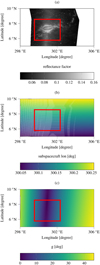 |
Fig. 1 Results from different processing steps for image M1147545058CE. The red rectangle marks the region of interest for the oval part of Reiner Gamma, (a) Radiance image after automos step, (b) Sub-spacecraft longitude in degrees for the odd image after the campt step in ISIS reprojected to input longitude and latitude values. The white lines represent missing data where no ground intersection can be calculated by ISIS for the odd image, (c) Phase angle after the step of angle calculation in Fig. 2. |
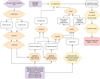 |
Fig. 2 Pipeline to radiometrically calibrate and geo-reference WAC images. The output is an image where each pixel location is defined in the coordinate system of the global WAC mosaic and the GLD100 DTM, and the angles i, e, and g are given for each pixel are based on the SPICE kernels. Purple denotes external data input. Orange denotes steps carried out in ISIS. Yellow denotes steps implemented in MATLAB or Python. |
2.3 Hapke model
The Hapke (2012b) model is a widely used radiative transfer model for particulate planetary surfaces. In general, it is empirical, but the parameters are physically motivated such that they can be interpreted as physical properties of the regolith. For a detailed description of the model, see Appendix A, Hapke (2012b), and Sato et al. (2014). The parameters of the Hapke model are, on the one hand, either geometric (incidence angle, i, emission angle, e, or phase angle, g) or, on the other hand, physical (single scattering albedo, w, phase function parameters, b and c, opposition effect strength, BS 0, and width, hs, as well as surface roughness,  ).
).
The opposition effect is related to the compaction of the regolith and leads to a strong peak for small phase angles; however, for typical lunar surfaces, this effect is still measurable at larger phase angles. The width of the opposition surge is modeled by the parameter hs, and the amplitude is denoted as BS 0. A compact surface generally appears brighter compared to the highly porous fairy castle structure usually found on the Moon, but the opposition effect is less strong because there are fewer shadows that could disappear for small phase angles. This typical correlation between albedo and opposition effect amplitude is empirically described by Sato et al. (2014) for the Moon with
 (1)
(1)
where the parameters s and t are derived for the different wavelengths of the WAC channels. For the 604 nm wavelength channel used in this work, s = 2.438 and t = 0.096. These values were also used for the NAC images because 604 nm is in the middle of the 400–760 nm sensitivity range of the camera. By dividing the estimated value by this predicted value, a corrected value can be obtained that gives insight into whether the estimated value is abnormal compared to the average lunar regolith, namely, smaller or larger compared to the average BS 0 for this albedo:
 (2)
(2)
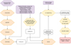 |
Fig. 3 Pipeline to radiometrically calibrate and geo-reference NAC images. The output is an image where each pixel corresponds to the pixel in the reference image M1114519536 and the angles i, e, and g for each pixel are based on the SPICE kernels. Purple denotes external input data. Orange denotes steps carried out in ISIS. Steps shown in yellow were implemented in MATLAB or Python. |
2.4 Bayesian model
Certain parameters of the Hapke (2012b) model are interdependent (e.g., w and BS 0) and some are even mathematically coupled, such as the parameters of the phase function b and c (e.g., Helfenstein 1986; Schmidt & Fernando 2015). Therefore, there are multiple solutions that can explain measured values equally well. The usage of conventional optimization techniques to invert the Hapke model may return best-fit values, but ignoring all other solutions that fit equally well. It is important to be aware of these uncertainties to be able to choose parameters that can be determined reliably based on the available image data. One technique that is well suited for these kinds of problems is Bayesian inference because the parameter space is thoroughly explored, and we obtain uncertainties complementary to the best-fit values. Because of the nonlinearities of the model and the not necessarily normally distributed parameters, we used Markov chain Monte Carlo (MCMC) sampling to numerically estimate the posterior probability density function (PDF) of the parameters, instead of solving the problem analytically.
Choosing a suitable likelihood function is inarguably the most important part of the Bayesian modeling approach. The likelihood is evaluated by comparing the model results for a certain set of parameters to the measured data. If the modeled results and the measured data fit well, then it is likely that the data originated from these parameters. To be able to distinguish the effects of the albedo and the other parameters more easily, we additionally used phase ratio information. For M images, we defined the measurements as a vector, R, of the length of M. The first image is preferentially a medium phase angle image without any shadows. The phase ratios used in this work were the pixel-wise ratios R1/R2…M between the reflectances of the first image divided by the reflectances of the remaining images and calculating the base-10 logarithm. This phase ratio vector has the dimension M − 1. Subsequently, we combined both by concatenation to obtain the final (2M − 1) × 1 data vector:
![Mathematical equation: ${{\bf{R}}_{{\rm{meas}}}} = \left[ {{{\bf{R}}_{M \times 1}},{{\log }_{10}}{{\left( {{{{R_1}} \mathord{\left/ {\vphantom {{{R_1}} {{{\bf{R}}_{2 \ldots M}}}}} \right. \kern-\nulldelimiterspace} {{{\bf{R}}_{2 \ldots M}}}}} \right)}_{\left( {M - 1} \right) \times 1}}} \right]. $](/articles/aa/full_html/2023/06/aa46098-23/aa46098-23-eq4.png) (3)
(3)
Assuming Gaussian noise, it is reasonable to select a normal distribution as the likelihood function. The normal distribution we selected had its mean at the modeled values and was evaluated for the measured values. The standard deviation of the likelihood function is an additional parameter of the model itself. Since the smaller the standard deviation, the higher the probability can become, and this has a strong effect. It should be noted that the reflectance values and the phase ratio values are of different orders of magnitude. Therefore, we included two different standard deviations as part of the model. We denoted the standard deviation for the reflectance part as σrefl and, for the phase ratio part, as σpr. Thus, we defined the standard deviation vector σlh of the likelihood function as:
![Mathematical equation: ${\sigma _{{\rm{lh}}}} = \left[ {{\sigma _{{\rm{refl}}}}\,{{\bf{1}}_{M \times 1}},{\sigma _{{\rm{pr}}}}{{\bf{1}}_{\left( {M - 1} \right) \times 1}}} \right],$](/articles/aa/full_html/2023/06/aa46098-23/aa46098-23-eq5.png) (4)
(4)
where 1M×1 is a vector of dimension, M, containing only ones. So the likelihood was evaluated for all observed and modeled values individually and is subsequently marginalized. Using the definitions above, the likelihood becomes:
 (5)
(5)
In addition, we included information on priors. The Hapke model has many parameters and not all of them can be simultaneously determined in a reliable way. The single scattering albedo, w, which is the main parameter of the Hapke model, is physically limited to the interval between zero and one. We chose an uninformative prior with a Beta distribution evenly distributed between zero and one as:
 (6)
(6)
The opposition effects are collected in a correction term based on the width, hs, and the strength, BS 0. The width is set to a fixed parameter according to Table 1. According to Sato et al. (2014), BS 0 is mainly distributed between 1.5 and 2.1. While in theory the amplitude is limited to the interval [0, 1] because both opposition effect terms are combined in BS, the amplitude is usually larger than 1. The parameter should not become negative so that we chose a log-normal distribution as a prior. In order to not overly penalize small values, we set the mean of the prior to e0.4 ≈ 1.5 and the standard deviation to 0.7. Thus, we have:
 (7)
(7)
The surface roughness,  , has a very weak effect for roughness angles below 10 degrees and is rarely larger than 40 degrees. Therefore, we set the prior distribution to be equally distributed between 10 and 50 degrees by using a scaled Beta distribution:
 (8)
(8)
Besides the physical parameters of the model, the standard deviation of the likelihood distribution is also a free parameter. It is common practice to use a half-normal distribution for the prior of the standard deviation such that
 (9)
(9)
 (10)
(10)
The parameters b and c of the phase function influence the shape of the phase curve and determine if the particles are forward or backward scattering and inherently follow the hockey stick relation (e.g., Hapke 2012a; Schmidt & Fernando 2015), which is given by Sato et al. (2014) as  . The parameter b is limited to the interval [0, 1]. Therefore, we again chose an uninformative Beta distribution as a prior for b.
To ultimately decide which parameters can be estimated, we designed an experiment where we estimated the uncertainties of the parameters given data synthetically generated with the Hapke model and a conservative estimate of the noise level (Gaussian noise with σn = 0.001). The observational geometry was selected to represent the data available for the central oval of Reiner Gamma. Given the nine observations, each with the nominal angles i, e, and g, we calculated the reflectance values for w = 0.3,  degrees, BS 0 = 1.7, hs = 0.11, b = 0.21, and c = 0.619. The signal-to-noise ratio (S/N) is approximately 77.7 compared to >42 for NAC imagery, for example, not considering the radiometric accuracy. These reflectance values were then used to invert the Hapke model to determine the parameters by employing the Bayesian method outlined in this section. Figure 4 shows the results when the b parameter of the phase function is free and c is set according to the hockey stick relation (Hapke 2002). The results indicate that the phase function parameters cannot be determined reliably. All solutions between strongly backscattering and forward scattering are accepted. Comparing those results to the results when the phase function is fixed (see Fig. 5) visualizes that the uncertainties of all free parameters can be reduced significantly if the value for b is constant. Additionally, in situations where the mean deviates strongly from the actual value (yellow diamond) in Fig. 4 it fits well for Fig. 5. In practice, using b as a free parameter for the actual data often resulted in multimodal posterior distributions for w, b, and c, making the mean an unreliable measure to describe the distribution. As illustrated by the results, the parameter has only a limited influence on the reflectance values. The shape of the phase function simply does not change significantly enough to be able to distinguish variations in b. Figure 6 shows some examples of solutions that might possibly be accepted by the Bayesian inference sampling even for the very narrow confidence band. In this example, a strongly backward-scattering but low-albedo material fits the data equally well as a forward-scattering material with higher albedo because there is not enough angular coverage to constrain the model. The other parameters in the example in Fig. 6 are constant. This is an indication that variations in b and c between, for instance, the swirl and its surroundings, cannot explain the photometric differences we observe in this study. Therefore, we decided to fix the b and c values according to Warell (2004) and infer the values of w, BS 0, and
  from the data. The parameter choices and corresponding priors are listed in Table 1.
The posterior distribution is then estimated by exploring the parameter space and sampling points until the samples converge to the posterior distribution. The No-U-Turn sampler (NUTS, Hoffman & Gelman 2014) was used to sample from the posterior distribution. NUTS is a very efficient algorithm that is widely used in Bayesian applications. We used the implementation of NUTS in pymc3 (Salvatier et al. 2016) and sampled 5000 tuning steps to set the individual step size, drawing two chains of each 20000 samples to make sure that the samples converge to the posterior density.
Parameters of the Hapke model and their values or estimation methods.
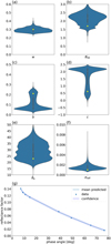 |
Fig. 4 Posterior distribution (a−f) of Hapke parameters given the reflectance values for the average angles of the observations at the central oval of Reiner Gamma with additive gaussian noise with a standard deviation of σn = 0.001. Panel (g) shows the posterior predictive values with a mean and confidence interval, which represents the standard deviation of all accepted samples. Yellow diamonds mark the theoretical input values used to generate the phase curve. |
3 Results
In this study, we want to investigate two regions with respect to their photometric behavior and compare their characteristics. First, we looked at the Chang’e-5 landing site at approximately 43.1°N and 51.8°W (see Sect. 3.1) in the northern part of Oceanus Procellarum near Mons Rümker (Zhou et al. 2022). This is an interesting study site because it offers the rare opportunity to investigate the photometric changes caused by a landing rocket jet because high-resolution NAC images from before and after the landing are available. Second, lunar swirls are still not fully understood and the Reiner Gamma swirl (see Sect. 3.2) is a prime research target as it is the most prominent representative of lunar swirls.
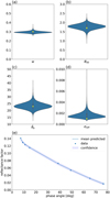 |
Fig. 5 Posterior distributions (a−d) of the Hapke parameters for the same phase curve as in Fig. 4, when the parameters b and c of the phase function are set to 0.21 and 0.619, respectively. Panel (e) shows the confidence interval of the posterior predictive values. |
3.1 Chang’e 5 landing site
The Chinese lunar mission Chang’e-5 landed successfully on December 1st, 2020, at approximately 43.1°N and 51.8°W. It collected a number of samples and the ascending stage lifted off two days later and returned to Earth (Zhou et al. 2022). The context of the landing site is shown in Fig. 7, where the region of interest evaluated in this study is marked by the red rectangle. The area is characterized by a typical mare terrain with small craters scattered around. The landing site is salient by three small craters in a triangular pattern, where the craters are smaller than 10 m in diameter, as can be seen in Fig. 7b.
The modeling results for image data acquired before the landing are shown in Fig. 8 as the mean predicted values (a−d), and the associated uncertainties are displayed as the standard deviation of the posterior distribution (e−h). The mean albedo of the area is 0.18, with no reliable values above 0.22. The roughness is overall small (mean over the area is 17.5 degrees) compared to the value in Sato et al. (2014), where a global mean value of 23.4 degrees was derived. In the maps of the roughness and the opposition effect amplitude, the craters are associated with higher values but are also associated with worse fits (Fig. 8d) and higher uncertainties (Figs. 8f and g). The mean BS 0 value over the area is 0.90 and, therefore, smaller than the values predicted for the derived low albedo. After the landing, the lander itself is visible in the albedo map as a bright spot between the three craters (Fig. 9a). The albedo increases significantly around the lander compared to before the landing (Fig. 8a). The surface roughness and the opposition effect are both reduced immediately around the lander, as can be seen in Figs. 9b and c in a similar pattern as the albedo has increased. Because of the Moon’s orbit, the images are all illuminated from the east or the west but never from the north or south. Therefore, the shadows of the lander in the image are also cast in these directions. These shadows can be seen in the maps of the mean predicted parameters (Fig. 9) as increased values in BS 0 and  and as higher uncertainties for all parameters as a bright line in the center of the image. Higher values of BS 0 and
  , in general, are also associated with higher uncertainties, just as craters are (again) not as well constrained. The uncertainties in the craters also stem from shadows at the eastern and western edges of the crater, often leading to the two semi-circles with higher uncertainties and higher values visible in the BS 0 and
  maps (see Figs. 8 and 9).
Using the correlation from Sato et al. (2014), the BS 0,corrected values are displayed in Fig. 10 for before and after the landing. A comparison of the two maps shows that the background has not changed significantly, but a strong negative anomaly can be Observed around the lander.
Based on the albedo, which does not exceed 0.22 before the landing, we could segment the region of interest into an area that was affected by the landing (w > 0.22) and an area that was not (or at least less so). This segment acts as a background (w < 0.22). We also defined pixels for which the standard deviation of the likelihood function σrefl exceeds 0.004 as unreliable and omit them from our analysis. This segmentation is shown in Fig. 11.
Subsequently, this segmentation can be used to plot the histograms of BS 0,estimated and BS 0,corrected for the two regions (Fig. 12). In Fig. 12a, the BS 0,estimated values and in Fig. 12b the corrected values are displayed, both before the landing. The corrected values are generally below one (roughly normally distributed around approximately 0.53) even though we would not have expected this region to have an abnormally weak opposition effect. The histograms of the study sites show that the BS 0 values after the landing (Figs. 12c,d) are generally also small. The segmentation, however, clearly shows that the values of BS 0,corrected in the area affected by the lander, are excessively small, corresponding to less than one-third of the typical values of lunar regolith with a comparable albedo. The mean of the background pixels is also smaller, with 0.45 compared to 0.53 before the landing. The segmentation discretely classifies pixels as “landing site” or “background”. However, the affected area actually has a diffuse boundary. Therefore, it can be stated that background pixels are also affected, even though to a lesser degree compared to the landing site. Consequently, the mean opposition effect strength of the background pixels is also slightly reduced compared to before the landing. The histograms of the two areas, landing site and background, appear to describe systematically different distributions. The mean of the BS 0,corrected values from the landing site is 0.28, compared to the background value of 0.45 after the landing. The Kolmogorov-Smirnow test (KS-test) statistics for the BS 0,estimated values of the two regions is D = 0.527 (p = 1.8 × 10⁻¹⁵) and for the BS 0,corrected values it is D = 0.511 (p = 1.8 × 10⁻¹⁵). The null hypothesis can thus be rejected.
The histograms for the roughness angle  are shown in Fig. 13 for before and after the landing. Before the landing, the roughness was overall higher with a mean of 17.5 degrees. After the landing, the background pixels appear to be only slightly affected by the landing rocket jet as the mean decreases to 17.2 degrees. The pixels classified as landing site show a reduced average roughness of 13.4 degrees. The modes of the two histograms, background and landing site, are very close to each other (12.5 and 11.6 degrees for background and landing site, respectively) and both are small compared to the mode before the landing, which was 14.7 degrees. The KS-test score is D = 0.436 (p = 1.78 × 10⁻¹⁵), suggesting that the effect is not as large as for the opposition effect but still both regions are systematically different.
 |
Fig. 6 Confidence interval from Fig. 4 with some exemplary reflectance phase curves. Both strongly backscattering and forward-scattering material can fit into the confidence interval and could be considered acceptable solutions given the noise level. The shape of the phase curve only changes marginally across the accessible range of phase angles. |
3.2 Reiner Gamma swirl
The Reiner Gamma swirl is centered at 7.5°N and 59.0°W in western Oceanus Procellarum, slightly north of the lunar equator. It is the most prominent example of these high-albedo anomalies found on the Moon that are commonly termed lunar swirls.
In the albedo map of the central oval part of the Reiner Gamma swirl, the bright albedo pattern is clearly visible (Fig. 14a). The roughness map (Fig. 14b) shows that the values are relatively noisy, and the uncertainties are high with several degrees and even exceed 10 degrees for some craters (Fig. 14f). A small difference can be observed for the dark lane in the northern oval, which exhibits a higher roughness. In the BS 0 map, however, the silhouette of the swirl can be distinguished by a weaker opposition effect amplitude. Craters, in turn, often coincide with weak BS 0 anomalies but are mostly related to higher uncertainties. The standard deviation of the likelihood function is higher for the craters (Fig. 14), indicating that the fit is worse, just as the uncertainties of all parameters are higher (Fig. 14). The results for the tail part are very similar to the central oval and are shown in the Appendix (Fig. D.1). The opposition effect strength is clearly smaller for the tail, even after correcting for the general correlation between albedo and BS 0 (Fig. D.2a). For the roughness in Fig. D.1b a very weak reduction can be observed at some locations, such as in the northernmost and southernmost parts of the tail.
When the dependence on albedo is removed from the opposition effect amplitude, the outlines of the swirl can still be clearly differentiated (Fig. 15a). The area can be segmented into on-swirl pixels with a higher albedo and off-swirl locations that represent the surrounding background mare. The albedo threshold is set to 0.21 and locations with σrefl > 0.004 are labeled as invalid. With this segmentation, the histograms of the estimated and corrected values are shown in Fig. 16. The BS 0,estimated values for the off-swirl pixels are mostly normally distributed around 1.75, and for the on-swirl locations, the mean is 1.37. On the other hand, the off-swirl BS 0,corrected values are almost exactly centered around 1.0, which means that they are on average exactly as predicted by Sato et al. (2014). In contrast, the on-swirl locations have a reduced opposition effect with an average BS 0,corrected value of 0.83. Because of the large number of locations in the distributions, the KS-test is significant with p = 0.00 for both corrected and estimated values. For the estimated values, the statistics is D = 0.539 and for the corrected values the difference is smaller between the on-swirl and off-swirl distributions. Consequently, D = 0.422 is also smaller. This dichotomy between on-swirl and off-swirl locations is even more pronounced for the tail region of Reiner Gamma. The segmentation for the tail is shown in Fig. D.2b, and the resulting histograms are in Fig. D.3. For that part of the swirl, the KS-test statistics are D = 0.725 and D = 0.607 for the estimated and corrected values, respectively. The difference between the roughness values on-swirl versus off-swirl is negligible with D = 0.075 (p = 3.98 × 10⁻³³) for the central oval and D = 0.071 (p = 6.88 × 10⁻⁹) for the tail.
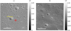 |
Fig. 7 Chang’e-5 landing site. Region of interest used in this study marked by the red rectangle in (a) shown in (b). The background image is LROC NAC frame M1114519536 centered at approximately 43.05°N and 51.95°W in (a). The larger crater to the northwest of the landing site is the Xu Guangqi crater (below the yellow label). |
4 Discussion
The bright regions of the Chang’e-5 landing site and the Reiner Gamma swirl show similar photometric behavior. Compared to the immediate surroundings, the albedo is increased, and the opposition effect is weaker in both cases. Additionally, at the landing site, the roughness is significantly reduced compared to the pre-landing surface, whereas a reduction of swirl roughness is barely discernible. The differences in opposition effect are similar for the landing site and swirl when compared to their respective surroundings, but the absolute values are excessively small at the landing site.
The strongly reduced BS 0 values at the landing site might be attributed to unsuitable standard parameters considered for the region. For example, the width, hs, of the opposition effect could be smaller at higher latitudes, but according to the maps of Sato et al. (2014), the width is almost constant within western Oceanus Procellarum (approx. 0.05 at both locations). Xu et al. (2022) found that the regolith at the landing site is more forward scattering compared to typical lunar regolith, which could also influence the estimated absolute BS 0 values. Since, for the landing site, only images at medium-to-large phase angles are available, the opposition effect is not fully constrained, as can be seen by the mean standard deviation of 0.7 over the landing site area before the landing and 0.51 after the landing, compared to 0.22 for the oval part of Reiner Gamma. The relative differences are still, however, strongly pronounced for the landing site. Importantly, the changes from the before to the after images show that a physical modification of the regolith structure has occurred.
This supports the findings of previous studies that the landing of a rocket on the lunar surface disturbs the microstructure of the regolith and leads to the destruction of the fairy castle structure, effectively making the regolith more compact (Kreslavsky & Shkuratov 2003; Clegg-Watkins et al. 2016). Xu et al. (2022) investigated a very small area around the Chang’e-5 lander and set the opposition effect and roughness parameters to constant values. Therefore, the results presented in this work are not directly comparable to Xu et al. (2020). Whether the observed behavior is due to a reduced shadow hiding opposition effect or more forward-scattering material cannot be reliably determined with NAC imagery. To effectively constrain the b and c parameters of the phase function, images acquired at phase angles well beyond 90 degrees are needed.
The presence of craters at both the landing site and the swirl coincide with higher uncertainties. The shape of the high uncertainty regions is not round as in the case of the crater but often split into two areas, one to the east and one to the west. The source of these uncertainties are shadows in large phase angle images. Considering the topography at each crater location alone, there should be light reflected even at the large phase angles. However, because of the crater topography, these regions are shadowed so that the model cannot adequately explain the large phase angle images, leading to higher uncertainties. In a qualitative analysis using only phase ratio images or in a modeling study with a classical least squares optimization, these areas would have to be carefully removed by hand, but because we are aware of the uncertainties, we can automatically omit them from the subsequent analysis.
The Reiner Gamma swirl consistently shows a reduced opposition effect strength, which is commonly interpreted to correspond to a more compact surface. At the landing site, we observed a similar behavior, and we know that the regolith has become more compact due to the rocket jet that blows away the porous top layer of the regolith. When comparing the Chang’e-5 landing site with the Reiner Gamma swirl, we find that both show a difference in compaction between the bright areas and the background. The difference found in opposition effect strength amounts to more than just the variation associated with albedo differences, suggesting that there must be a physical difference between the surface microstructure of bright and dark areas. The mean predicted roughness at the Reiner Gamma swirl shows only very weak anomalies correlated with the swirl albedo, whereas the landing site shows a more strongly reduced roughness. Shkuratov et al. (2010) theorized that the influence of multiple scattering of immature soils might counteract roughness effects. The gas pressure at the landing site is approximately 170 Pa on average in the exit plane and around 420 Pa at the nozzle wall (Zhang et al. 2022). At the swirls, Starukhina & Shkuratov (2004) calculated that a passing cometary coma creates pressures in the broad range of 40–400 Pa at the surface. Both regions exhibit pressures of a similar order of magnitude. The reduced roughness at the landing site is only visible in a small area around the lander of less than 20 m from the lander, where the pressure from the exhaust was highest. Possibly, the pressure of a cometary coma is closer to the lower end of the range and, therefore, not high enough to completely remove a regolith layer and transport it over much larger distances, but only to compact it without a significant change of the surface roughness. Additionally, the Chang’e-5 mission included an ascending stage that disturbed the surface structure of the regolith for a second time. Despite the presumably slightly higher exhaust pressure, the decrease in roughness is as small as 4 degrees (around 20%) or less at the landing site compared to before the landing.
Three mechanisms might be considered to play a role in the appearance of lunar swirls: (1) reduced or abnormal space weathering due to magnetic shielding (e.g., Trang & Lucey 2019; Blewett et al. 2021); (2) sorting of grains by electric or magnetic fields (e.g., Garrick-Bethell et al. 2011); and (3) interaction of a cometary coma with the surface (e.g., Schultz & Srnka 1980; Pinet et al. 2000; Starukhina & Shkuratov 2004; Syal & Schultz 2015; Hess et al. 2020a). The spectral characteristics of swirls can, to a large extent, be explained by abnormal space weathering. This means that swirls lack nanophase iron (npFe) particles but there is no deficiency in larger microphase iron (mpFe) particles (Trang & Lucey 2019; Blewett et al. 2021). However, this does not explain the photometric differences found between the swirl and its surroundings. Therefore, a difference in compaction or grain size should still be considered a contributing factor. The individual contributions of the various processes might be different depending on the area. The spectral significance of compaction defined by Hess et al. (2020a) is higher in the northeastern tail region of the Reiner Gamma swirl, compared to the central oval. This is also consistent with the results presented in this work, where the difference between the opposition effect strength of the swirl and the surrounding terrain is more pronounced for the tail region.
Also, the grain size strongly contributes to the observed spectral and Polarimetrie properties of the lunar regolith (e.g., Bhatt et al. 2023), but the grain size variation cannot be constrained based on photometric data alone. If the surface at swirls was enriched with finely grained feldspathic dust by electrostatic sorting as proposed by Garrick-Bethell et al. (2011), the spectral effect would be similar to higher compaction and could lead to a reduced roughness as well. However, the forces might not be strong enough to significantly alter the surface structure to have an influence on the surface roughness. While most swirls are co-located with magnetic anomalies, there is a swirl structure in the Mare Moscoviense basin that is not protected by a magnetic field (e.g., Hess et al. 2020a) that would be required to create the electric field responsible for the sorting of dust. A general swirl formation mechanism has to be able to explain these occurrences as well.
The photometric observations favor the interpretation that swirls are created by some interactions between a comet’s coma and the lunar surface (Shevchenko 1993; Pinet et al. 2000; Syal & Schultz 2015). On the one hand, this could be attributed to the effects of the coma of an impacting comet. For example, Syal & Schultz (2015) showed that such a coma could cause scouring at scales of lunar swirls and can also explain the complex shapes. On the other hand, the passing of a comet and the interaction of the inner, denser parts of the coma with the surface would cause an effect similar to a landing rocket jet (Shevchenko 1993). The parts of a coma dense enough to be able to alter the physical surface properties are less than 1000 km in radius (Syal & Schultz 2015) and could explain the extent of Reiner Gamma, which has a length of roughly 300 km and a width of 45 km at the central oval. Magnetic shielding can preserve swirls by reducing the solar wind influx so that the surface does not become mature and more porous as quickly as the unshielded surface, which would mean that the Mare Moscoviense swirl not associated with a magnetic field is younger than other swirls (Hess et al. 2020b).
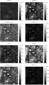 |
Fig. 8 Results for the Chang’e-5 landing site before the landing. Means of the posterior distributions (a−d) for the parameters w, |

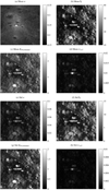 |
Fig. 9 Results for the Chang’e-5 landing site after the landing. Means of the posterior distributions (a−d) for the parameters w, |

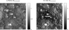 |
Fig. 10 Comparison of BS 0 corrected for the influence of albedo according to Eq. (2) between before and after the landing. |
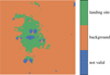 |
Fig. 11 Segmentation of the region of interest after the landing into an area strongly influenced by the rocket jet (landing site) and not as clearly influenced by the landing (background). Areas with a mean predicted albedo w above 0.22 are denoted as landing site. Areas with a mean predicted σ above 0.004 are labeled as invalid because the uncertainties are too high. Consequently, these areas are excluded from the analysis of the landing site and background regions. |
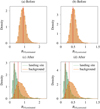 |
Fig. 12 Histograms of BS 0,estimated and BS 0,corrected for before and after the landing. For after the landing, two separate distributions for the landing site and background are shown. The modes of the histograms are indicated by the red vertical lines. |
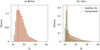 |
Fig. 13 Histograms of the roughness angle |

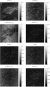 |
Fig. 14 Results for the oval region of the Reiner Gamma swirl. Means of the posterior distribution for the Hapke model parameters w, |

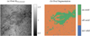 |
Fig. 15 Maps of the corrected BS 0 value to remove the dependence on albedo (a). Segmentation of the region of interest based on the mean albedo (b). Areas with an albedo larger than 0.21 are labeled as on-swirl. Areas with a mean predicted σ above 0.004 are labeled as invalid as the uncertainties are too high. |
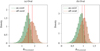 |
Fig. 16 Distribution of (a) BS 0,estimated and (b) BS 0,corrected for on-swirl and off-swirl areas according to Fig. 15b. The modes of the histograms are indicated by red vertical lines. |
5 Conclusion
We introduce a Bayesian framework to estimate the Hapke photometric parameters and their uncertainties. Depending on the available data, a suitable model can be chosen and either of the following concerns can be directly inferred: which of the parameters are reliable, what additional data are required to improve the estimation accuracy, or which parameters are difficult to estimate or are mutually interrelated. In this way, the interpretation of the results can be focused on the areas with higher confidence.
We applied this framework to the Chang’e-5 landing site and the Reiner Gamma swirl. Both regions exhibit excessively weak opposition effects and an increased albedo. The reduction of the opposition effect amplitude goes well beyond the expected value for typical lunar regolith of similar albedo, suggesting that the physical properties of the regolith are also distinct. For the landing site (which additionally exhibits clear characteristics of reduced roughness), this optical change is a direct consequence of the top regolith layer having been blown away by the descent and ascent rocket jets, leaving behind a more compact and smoother surface. At swirls, this difference between the swirl and its surroundings could be attributed to changes caused by a cometary coma acting similarly to a landing rocket jet. There appears to be a minor difference between the roughness of the swirl and the surroundings, but the difference is statistically not significant when compared to the uncertainties. This behavior might be attributed to slight differences in gas pressure between the swirl and the landing site, where the pressure was presumed to be relatively high so close to the lander. A cometary coma might not generate enough pressure to alter the surface roughness, but it could still destroy the fairy castle structure of the regolith and increase its compaction. The magnetic shielding would then serve as a preservation mechanism resulting in immature surface regolith, with a fairy castle structure building up more slowly at the swirls than in the surrounding mare.
Acknowledgements
We want to thank the LROC team and NASA/JPL for making the NAC and WAC images publicly available on the PDS.
Appendix A Hapke model
This section closely follows the parameter definitions in Sato et al. (2014). The general observation geometry is given by the emission angle, e, between the observation direction, υ, and surface normal, n. The incidence angle, i, is the angle between the vector pointing to the sun, s, and the surface normal, n. Finally, the phase angle, g, is the angle between the directions of incidence, s, and emission, υ. Hapke (2012b) formulated the isotropic multiple scattering approximation (IMSA) as follows:
![Mathematical equation: $r\left( {i,e,g} \right) = {\omega \over {4\pi }}{{{\mu _{0,e}}} \over {{\mu _e} + {\mu _{0,e}}}}\left[ {p\left( g \right){B_{S\,H}}\left( g \right) + H\left( {{\mu _e}} \right)H\left( {{\mu _{0,e}}} \right) - 1} \right]\,S\,\left( {i,e,\psi } \right),$](/articles/aa/full_html/2023/06/aa46098-23/aa46098-23-eq24.png) (A.1)
(A.1)
where w denotes the single scattering albedo, which is the main parameter of the Hapke model. The material-dependent single particle phase function p(g) defines how much incident light is scattered in a forward or backward direction. A common choice for this computation is the double Henyey-Greenstein function
 (A.2)
(A.2)
with two parameters b and c, where c is positive for more backward-scattering particles and negative for more forward-scattering particles. Parameter b describes the shapes of the scattering lobes.
Under small phase angles (or in opposition) the surface appears brighter than expected. This is due to the geometrical effect that small shadows in the microstructure of the surface disappear, but also due to coherent backscattering effects. Because shadow hiding and coherent backscatter cannot be disentangled, both opposition effects can be collected in the shadow-hiding opposition-effect term (Warell 2004):
 (A.3)
(A.3)
The incidence and emission angles mainly appear by their cosine values:
 (A.4)
(A.4)
However, to account for the effects of surface roughness, effective angles, ie and ee, and their cosine values, µ0,e and µe, must be used, and a correction term S (i, e, g) is defined. Two cases have to be distinguished. For i < e:
 (A.5)
(A.5)
 (A.6)
(A.6)
 (A.7)
(A.7)
For i ≥ e:
 (A.8)
(A.8)
 (A.9)
(A.9)
 (A.10)
The helper functions for both cases are defined as follows. The function χ is defined as
 (A.11)
and the function η as
 (A.12)
with
 (A.13)
 (A.14)
and
 (A.15)
with the azimuth angle
 (A.16)
Multiple scattering within the medium is modelled by Chandrasekhar’s H-function using the updated approximation from Hapke (2002) given by
![Mathematical equation: $H\left( x \right) = {\left[ {1 - wx\left( {{r_0} + {{1 - 2{r_0}x} \over 2}\ln \left( {{{1 + x} \over x}} \right)} \right)} \right]^{ - 1}},$](/articles/aa/full_html/2023/06/aa46098-23/aa46098-23-eq40.png) (A.17)
(A.17)
with
 (A.18)
Appendix B Probability distributions
B.1 Beta distribution
The beta distribution is limited to the interval [0, 1] and is defined as
 (B.1)
(B.1)
with
 (B.2)
(B.2)
Some example distributions are shown in Fig. B.1. For α = 1 and β = 1 the PDF is equally distributed between zero and one. If α and β are larger than one the distribution has a single mode at  . It is bimodal if α and β are both below one.
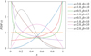 |
Fig. B.1 Examples of a beta distribution. |
B.2 Log-normal distribution
The log-normal distribution is given by:
 (B.3)
(B.3)
and is only valid for positive values of x. The mean of the distribution is at log(µ). For example, for µ = 0 the mean is 1. Some examples are shown in Fig. B.2. The variance is given by
 (B.4)
(B.4)
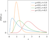 |
Fig. B.2 Examples of log-normal distributions for varying mean and standard deviation. |
B.3 Half-normal distribution
The half-normal distribution is a normal distribution with a mode at zero and all values below zero having zero probability.
It is defined as:
 (B.5)
(B.5)
An example distribution with a variance of 1 is shown in Fig. B.3.
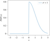 |
Fig. B.3 Example half-normal distribution. The mode is always zero but the variance is variable. |
Appendix C Data
NAC images taken before the landing of Chang’e-5.
NAC images taken after the landing of Chang’e-5.
WAC images used for analyzing the oval region of Reiner Gamma.
WAC images used for analyzing the tail region of Reiner Gamma.
Appendix D Reiner Gamma tail region
 |
Fig. D.1 Mean predicted values in the tail region of Reiner Gamma of: (a) single scattering albedo, w, (b) surface roughness, |

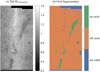 |
Fig. D.2 Corrected BS 0 to remove the influence of the albedo (a). Segmentation of the region of interest based on the mean albedo (b). Areas with an albedo larger than 0.21 are labeled as on-swirl. Areas with a mean predicted σ > 0.004 are labeled as invalid because the uncertainties are too high. |
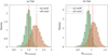 |
Fig. D.3 Distribution of (a) BS 0,estimated and (b) BS 0,corrected for on-swirl and off-swirl areas according to Fig. D.2b. The mean of BS 0,corrected is 0.87 for the on-swirl pixels and 1.08 for the off-swirl pixels. The KS-Test statistics are D = 0.725 (p = 0.000) for the estimated values and D = 0.607 (p = 0.000 for the corrected values between on-swirl and off-swirl. The modes of the histograms are indicated by the red vertical lines. |
References
- Belgacem, I., Schmidt, F., & Jonniaux, G. 2020, Icarus, 338, 113525 [NASA ADS] [CrossRef] [Google Scholar]
- Belgacem, I., Schmidt, F., & Jonniaux, G. 2021, Icarus, 369, 114631 [NASA ADS] [CrossRef] [Google Scholar]
- Bhatt, M., Wöhler, C., Rogall, J., et al. 2023, A & A, 674, A82 [NASA ADS] [CrossRef] [EDP Sciences] [Google Scholar]
- Blewett, D. T., Denevi, B. W., Cahill, J. T., & Klima, R. L. 2021, Icarus, 364, 114472 [NASA ADS] [CrossRef] [Google Scholar]
- Clegg-Watkins, R., Jolliff, B., Boyd, A., et al. 2016, Icarus, 273, 84 [NASA ADS] [CrossRef] [Google Scholar]
- Denevi, B. W., Robinson, M. S., Boyd, A. K., Blewett, D. T., & Klima, R. L. 2016, Icarus, 273, 53 [CrossRef] [Google Scholar]
- Domingue, D., Weirich, J., Chuang, F., Sickafoose, A., & Palmer, E. 2022, Geophys. Res. Lett., 49, e2021GL095285 [CrossRef] [Google Scholar]
- Fernando, J., Schmidt, F., Ceamanos, X., et al. 2013, J. Geophys. Res. Planets, 118, 534 [NASA ADS] [CrossRef] [Google Scholar]
- Fernando, J., Schmidt, F., Pilorget, C., et al. 2015, Icarus, 253, 271 [NASA ADS] [CrossRef] [Google Scholar]
- Garrick-Bethell, I., Head III, J. W., & Pieters, C. M. 2011, Icarus, 212, 480 [NASA ADS] [CrossRef] [Google Scholar]
- Glotch, T. D., Bandfield, J. L., Lucey, P. G., et al. 2015, Nat. Commun., 6, 1 [CrossRef] [Google Scholar]
- Grumpe, A., Belkhir, F., & Wöhler, C. 2014, Adv. Space Res., 53, 1735 [NASA ADS] [CrossRef] [Google Scholar]
- Grumpe, A., Wöhler, C., Berezhnoy, A. A., & Shevchenko, V. V. 2019, Icarus, 321, 486 [NASA ADS] [CrossRef] [Google Scholar]
- Hapke, B. 2002, Icarus, 157, 523 [NASA ADS] [CrossRef] [Google Scholar]
- Hapke, B. 2012a, Icarus, 221, 1079 [NASA ADS] [CrossRef] [Google Scholar]
- Hapke, B. 2012b, Theory of Reflectance and Emittance Spectroscopy (Cambridge: Cambridge University Press) [Google Scholar]
- Helfenstein, P. 1986, Lunar Planet. Sci. Conf., 17, 333 [Google Scholar]
- Hendrix, A., Greathouse, T., Retherford, K., et al. 2016, Icarus, 273, 68 [NASA ADS] [CrossRef] [Google Scholar]
- Hess, M., Wöhler, C., Bhatt, M., et al. 2020a, A & A, 639, A12 [NASA ADS] [CrossRef] [EDP Sciences] [Google Scholar]
- Hess, M., Wohlfarth, K., Wöhler, C., et al. 2020b, in Europlanet Science Congress 2020, 14 (Copernicus Meetings) [Google Scholar]
- Hoffman, M. D., & Gelman, A. 2014, J. Mach. Learn. Res., 15, 1593 [Google Scholar]
- Hood, L., & Schubert, G. 1980, Science, 208, 49 [NASA ADS] [CrossRef] [Google Scholar]
- Hood, L. & Williams, C. 1989, Lunar Planet. Sci. Conf. Proc., 19, 99 [Google Scholar]
- Kaydash, V., Kreslavsky, M., Shkuratov, Y., et al. 2009, Icarus, 202, 393 [NASA ADS] [CrossRef] [Google Scholar]
- Kramer, G. Y., Besse, S., Dhingra, D., et al. 2011, J. Geophys. Res. Planets, 116, E10 [CrossRef] [Google Scholar]
- Kreslavsky, M., & Shkuratov, Y. G. 2003, J. Geophys. Res. Planets, 108, E3 [NASA ADS] [CrossRef] [Google Scholar]
- Laura, J., Acosta, A., Addair, T., et al. 2022, https://doi.org/10.5281/zenodo.6950434 [Google Scholar]
- Li, S., & Garrick-Bethell, I. 2019, Geophys. Res. Lett., 46, 14318 [NASA ADS] [CrossRef] [Google Scholar]
- Lue, C., Futaana, Y., Barabash, S., et al. 2011, Geophys. Res. Lett., 38, 22 [Google Scholar]
- Pieters, C. M., & Noble, S. K. 2016, J. Geophys. Res. Planets, 121, 1865 [CrossRef] [Google Scholar]
- Pieters, C., Donaldson Hanna, K., Sunshine, J., & Garrick-Bethell, I. 2021, Lunar Planet. Sci. Conf., 2548, 1686 [Google Scholar]
- Pinet, P. C., Shevchenko, V. V., Chevrel, S. D., Daydou, Y., & Rosemberg, C. 2000, J. Geophys. Res. Planets, 105, 9457 [NASA ADS] [CrossRef] [Google Scholar]
- Pinet, P., Cord, A., Chevrel, S., & Daydou, Y. 2004, Lunar Planet. Sci. Conf., 35, 1660 [Google Scholar]
- Robinson, M., Brylow, S., Tschimmel, M., et al. 2010, Space Sci. Rev., 150, 81 [CrossRef] [Google Scholar]
- Salvatier, J., Wiecki, T. V., & Fonnesbeck, C. 2016, PeerJ Comput. Sci., 2, e55 [Google Scholar]
- Sato, H., Robinson, M., Hapke, B., Denevi, B., & Boyd, A. 2014, J. Geophys. Res. Planets, 119, 1775 [NASA ADS] [CrossRef] [Google Scholar]
- Sato, H., Robinson, M. S., Lawrence, S. J., et al. 2017, Icarus, 296, 216 [NASA ADS] [CrossRef] [Google Scholar]
- Schmidt, F., & Fernando, J. 2015, Icarus, 260, 73 [NASA ADS] [CrossRef] [Google Scholar]
- Scholten, F., Oberst, J., Matz, K.-D., et al. 2012, J. Geophys. Res. Planets, 117, E12 [Google Scholar]
- Schultz, P. H., & Srnka, L. J. 1980, Nature, 284, 22 [CrossRef] [Google Scholar]
- Shevchenko, V. 1993, Astron. Rep., 37, 314 [NASA ADS] [Google Scholar]
- Shevchenko, V., Pinet, P., & Chevrel, S. 1994, Sol. Syst. Res., 27, 310 [NASA ADS] [Google Scholar]
- Shkuratov, Y., Opanasenko, N., Zubko, E., et al. 2007, Icarus, 187, 406 [NASA ADS] [CrossRef] [Google Scholar]
- Shkuratov, Y., Kaydash, V., Gerasimenko, S., et al. 2010, Icarus, 208, 20 [NASA ADS] [CrossRef] [Google Scholar]
- Shkuratov, Y., Kaydash, V., Korokhin, V., et al. 2011, Planet. Space Sci., 59, 1326 [Google Scholar]
- Starukhina, L. V., & Shkuratov, Y. G. 2004, Icarus, 167, 136 [NASA ADS] [CrossRef] [Google Scholar]
- Syal, M. B., & Schultz, P. H. 2015, Icarus, 257, 194 [CrossRef] [Google Scholar]
- Trang, D., & Lucey, P. G. 2019, Icarus, 321, 307 [CrossRef] [Google Scholar]
- Tsunakawa, H., Takahashi, F., Shimizu, H., Shibuya, H., & Matsushima, M. 2015, J. Geophys. Res. Planets, 120, 1160 [NASA ADS] [CrossRef] [Google Scholar]
- Warell, J. 2004, Icarus, 167, 271 [NASA ADS] [CrossRef] [Google Scholar]
- Wieser, M., Barabash, S., Futaana, Y., et al. 2010, Geophys. Res. Lett., 37, 5 [Google Scholar]
- Xu, X., Liu, J., Liu, D., Liu, B., & Shu, R. 2020, Remote Sens., 12, 3676 [NASA ADS] [CrossRef] [Google Scholar]
- Xu, J., Wang, M., Lin, H., et al. 2022, Geophys. Res. Lett., 49, e2021GL096876 [Google Scholar]
- Zhang, H., Li, C., You, J., et al. 2022, Aerospace, 9, 358 [NASA ADS] [CrossRef] [Google Scholar]
- Zhou, C., Jia, Y., Liu, J., et al. 2022, Adv. Space Res., 69, 823 [NASA ADS] [CrossRef] [Google Scholar]
All Tables
All Figures
|
Fig. 1 Results from different processing steps for image M1147545058CE. The red rectangle marks the region of interest for the oval part of Reiner Gamma, (a) Radiance image after automos step, (b) Sub-spacecraft longitude in degrees for the odd image after the campt step in ISIS reprojected to input longitude and latitude values. The white lines represent missing data where no ground intersection can be calculated by ISIS for the odd image, (c) Phase angle after the step of angle calculation in Fig. 2. |
| In the text | |
|
Fig. 2 Pipeline to radiometrically calibrate and geo-reference WAC images. The output is an image where each pixel location is defined in the coordinate system of the global WAC mosaic and the GLD100 DTM, and the angles i, e, and g are given for each pixel are based on the SPICE kernels. Purple denotes external data input. Orange denotes steps carried out in ISIS. Yellow denotes steps implemented in MATLAB or Python. |
| In the text | |
|
Fig. 3 Pipeline to radiometrically calibrate and geo-reference NAC images. The output is an image where each pixel corresponds to the pixel in the reference image M1114519536 and the angles i, e, and g for each pixel are based on the SPICE kernels. Purple denotes external input data. Orange denotes steps carried out in ISIS. Steps shown in yellow were implemented in MATLAB or Python. |
| In the text | |
|
Fig. 4 Posterior distribution (a−f) of Hapke parameters given the reflectance values for the average angles of the observations at the central oval of Reiner Gamma with additive gaussian noise with a standard deviation of σn = 0.001. Panel (g) shows the posterior predictive values with a mean and confidence interval, which represents the standard deviation of all accepted samples. Yellow diamonds mark the theoretical input values used to generate the phase curve. |
| In the text | |
|
Fig. 5 Posterior distributions (a−d) of the Hapke parameters for the same phase curve as in Fig. 4, when the parameters b and c of the phase function are set to 0.21 and 0.619, respectively. Panel (e) shows the confidence interval of the posterior predictive values. |
| In the text | |
|
Fig. 6 Confidence interval from Fig. 4 with some exemplary reflectance phase curves. Both strongly backscattering and forward-scattering material can fit into the confidence interval and could be considered acceptable solutions given the noise level. The shape of the phase curve only changes marginally across the accessible range of phase angles. |
| In the text | |
|
Fig. 7 Chang’e-5 landing site. Region of interest used in this study marked by the red rectangle in (a) shown in (b). The background image is LROC NAC frame M1114519536 centered at approximately 43.05°N and 51.95°W in (a). The larger crater to the northwest of the landing site is the Xu Guangqi crater (below the yellow label). |
| In the text | |
|
Fig. 8 Results for the Chang’e-5 landing site before the landing. Means of the posterior distributions (a−d) for the parameters w, |
| In the text | |
|
Fig. 9 Results for the Chang’e-5 landing site after the landing. Means of the posterior distributions (a−d) for the parameters w, |
| In the text | |
|
Fig. 10 Comparison of BS 0 corrected for the influence of albedo according to Eq. (2) between before and after the landing. |
| In the text | |
|
Fig. 11 Segmentation of the region of interest after the landing into an area strongly influenced by the rocket jet (landing site) and not as clearly influenced by the landing (background). Areas with a mean predicted albedo w above 0.22 are denoted as landing site. Areas with a mean predicted σ above 0.004 are labeled as invalid because the uncertainties are too high. Consequently, these areas are excluded from the analysis of the landing site and background regions. |
| In the text | |
|
Fig. 12 Histograms of BS 0,estimated and BS 0,corrected for before and after the landing. For after the landing, two separate distributions for the landing site and background are shown. The modes of the histograms are indicated by the red vertical lines. |
| In the text | |
|
Fig. 13 Histograms of the roughness angle |
| In the text | |
|
Fig. 14 Results for the oval region of the Reiner Gamma swirl. Means of the posterior distribution for the Hapke model parameters w, |
| In the text | |
|
Fig. 15 Maps of the corrected BS 0 value to remove the dependence on albedo (a). Segmentation of the region of interest based on the mean albedo (b). Areas with an albedo larger than 0.21 are labeled as on-swirl. Areas with a mean predicted σ above 0.004 are labeled as invalid as the uncertainties are too high. |
| In the text | |
|
Fig. 16 Distribution of (a) BS 0,estimated and (b) BS 0,corrected for on-swirl and off-swirl areas according to Fig. 15b. The modes of the histograms are indicated by red vertical lines. |
| In the text | |
|
Fig. B.1 Examples of a beta distribution. |
| In the text | |
|
Fig. B.2 Examples of log-normal distributions for varying mean and standard deviation. |
| In the text | |
|
Fig. B.3 Example half-normal distribution. The mode is always zero but the variance is variable. |
| In the text | |
|
Fig. D.1 Mean predicted values in the tail region of Reiner Gamma of: (a) single scattering albedo, w, (b) surface roughness, |
| In the text | |
|
Fig. D.2 Corrected BS 0 to remove the influence of the albedo (a). Segmentation of the region of interest based on the mean albedo (b). Areas with an albedo larger than 0.21 are labeled as on-swirl. Areas with a mean predicted σ > 0.004 are labeled as invalid because the uncertainties are too high. |
| In the text | |
|
Fig. D.3 Distribution of (a) BS 0,estimated and (b) BS 0,corrected for on-swirl and off-swirl areas according to Fig. D.2b. The mean of BS 0,corrected is 0.87 for the on-swirl pixels and 1.08 for the off-swirl pixels. The KS-Test statistics are D = 0.725 (p = 0.000) for the estimated values and D = 0.607 (p = 0.000 for the corrected values between on-swirl and off-swirl. The modes of the histograms are indicated by the red vertical lines. |
| In the text | |
Current usage metrics show cumulative count of Article Views (full-text article views including HTML views, PDF and ePub downloads, according to the available data) and Abstracts Views on Vision4Press platform.
Data correspond to usage on the plateform after 2015. The current usage metrics is available 48-96 hours after online publication and is updated daily on week days.
Initial download of the metrics may take a while.