| Issue |
A&A
Volume 639, July 2020
|
|
|---|---|---|
| Article Number | A145 | |
| Number of page(s) | 10 | |
| Section | Extragalactic astronomy | |
| DOI | https://doi.org/10.1051/0004-6361/201935802 | |
| Published online | 27 July 2020 | |
Anisotropy of random motions of gas in Messier 33
1
Centro de Astronomía, Universidad de Antofagasta, Avda. U. de Antofagasta, 02800 Antofagasta, Chile
e-mail: laurent.chemin@uantof.cl, astro.chemin@gmail.com
2
Laboratoire d’Astrophysique de Bordeaux, Univ. Bordeaux, CNRS, B18N, Allée Geoffroy Saint-Hilaire, 33615 Pessac, France
3
Observatoire de Paris, LERMA, College de France, CNRS, PSL Univ., Sorbonne Univ., UPMC, Paris, France
4
Laboratoire de Physique et de Chimie de l’Environnement, Observatoire d’Astrophysique de l’Université Ouaga I Pr Joseph Ki-Zerbo (ODAUO), 03 BP 7021 Ouaga 03, Burkina Faso
5
Department of Astronomy, University of Cape Town, Private Bag X3, Rondebosch, 7701, South Africa
Received:
29
April
2019
Accepted:
19
May
2020
Context. The ellipsoid of random motions of the gaseous medium in galactic disks is often considered isotropic, as appropriate if the gas is highly collisional. However, the collisional or collisionless behavior of the gas is a subject of debate. If the gas is clumpy with a low collision rate, then the often observed asymmetries in the gas velocity dispersion could be hints of anisotropic motions in a gaseous collisionless medium.
Aims. We study the properties of anisotropic and axisymmetric velocity ellipsoids from maps of the gas velocity dispersion in nearby galaxies. This data allow us to measure the azimuthal-to-radial axis ratio of gas velocity ellipsoids, which is a useful tool to study the structure of gaseous orbits in the disk. We also present the first estimates of perturbations in gas velocity dispersion maps by applying an alternative model that considers isotropic and asymmetric random motions.
Methods. High-quality velocity dispersion maps of the atomic medium at various angular resolutions of the nearby spiral galaxy Messier 33, are used to test the anisotropic and isotropic velocity models. The velocity dispersions of hundreds of individual molecular clouds are also analyzed.
Results. The HI velocity dispersion of M 33 is systematically larger along the minor axis, and lower along the major axis. Isotropy is only possible if asymmetric motions are considered. Fourier transforms of the H I velocity dispersions reveal a bisymmetric mode which is mostly stronger than other asymmetric motions and aligned with the minor axis of the galaxy. Within the anisotropic and axisymmetric velocity model, the stronger bisymmetry is explained by a radial component that is larger than the azimuthal component of the ellipsoid of random motions, thus by gaseous orbits that are dominantly radial. The azimuthal anisotropy parameter is not strongly dependent on the choice of the vertical dispersion. The velocity anisotropy parameter of the molecular clouds is observed highly scattered.
Conclusions. Perturbations such as HI spiral-like arms could be at the origin of the gas velocity anisotropy in M 33. Further work is necessary to assess whether anisotropic velocity ellispsoids can also be invoked to explain the asymmetric gas random motions of other galaxies.
Key words: galaxies: fundamental parameters / galaxies: kinematics and dynamics / galaxies: spiral / galaxies: individual: Messier 33 (NGC 598, Triangulum)
© ESO 2020
1. Introduction
What is the structure of orbits in the interstellar medium of disk galaxies? What is the shape of the gaseous velocity dispersion ellipsoid in the mid-plane of galactic disks?
A quick look at observations of nearby galaxies is helpful to guess that orbits should not be perfectly circular, owing to the presence of large-scale perturbations like bars, spiral arms, warps, or disk lopsidedness. Rotational motions are accompanied by radial and streaming motions, and orbits become asymmetric (Kalnajs 1973; Visser 1980). In a galactic disk, the structure of orbits can be studied by means of the shape of the velocity dispersion ellipsoid σR, σϕ, and σz, which are respectively the radial, tangential, and vertical components of random motions in cylindrical coordinates. The ellipsoid is characterized by three axis ratios, one of which is the azimuthal-to-radial ratio that traces the degree of anisotropy in the mid-plane, as characterized by the azimuthal anisotropy parameter, βϕ = 1 − (σϕ/σR)2. Orbits that are biased tangentially have βϕ < 0, with βϕ → −∞ for circular orbits, whereas those biased radially have 0 < βϕ < 1 (Binney & Tremaine 2008). This parameter is appropriate to explain the orbital structure of a kinematic tracer that is collisionless (stars). We would expect to observe such values within gaseous disks of galaxies, if interstellar gas behaved partly like a collisionless medium, as shown in numerical models (Bottema 2003; Agertz et al. 2009).
Interstellar gas is a medium in which collisions and shocks coming from all directions are thought to completely “isotropize” the motions. Assuming a velocity ellipsoid that is not tilted, the line-of-sight dispersion can be written

where i is the disk inclination, ϕ the azimuthal angle in the disk plane, σT the thermal (isotropic) component, and σins the instrumental broadening. Isotropy greatly simplifies the modeling of the observed dispersion as it implies σR = σϕ = σz = σiso, reducing Eq. (1) to
Important values for galactic dynamics like the gas radial pressure support depending on σR (Dalcanton & Stilp 2010; Oh et al. 2015) or the vertical equilibrium depending on σz (Combes & Becquaert 1997; Koyama & Ostriker 2009; Bershady et al. 2010; Martinsson et al. 2013) can then be easily estimated directly from observations, without needing to deproject σlos.
The analysis of σlos is less straightforward in the hypothesis that part of the gas behaves as a collisionless medium. Equation (1) has to be modeled or inverted in order to fit or deproject (respectively) the data, and constrain the shape of the velocity ellipsoid. Moreover, Eq. (1) predicts that σlos is a function of the azimuthal angle owing to the projection of the radial and tangential components into σlos. In an axisymmetric approach of this kind, an anisotropic dispersion ellipsoid has a significant implication on σlos: it has to be asymmetric, greater near the minor (major) axis for σϕ < σR (σϕ > σR, respectively). To our knowledge, such strong prediction has never been tested. Many observed velocity dispersion fields exhibit asymmetric σlos dependent on the azimuth (Fig. 1, and Walter et al. 2008), and some of them are reminiscent of this particular anisotropic signature.
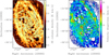 |
Fig. 1. Observational data of Messier 33. Left panel: HI column density map (VLA, 100 pc resolution, logarithmic stretch) with Spitzer/IRAC 3.6 μm stellar distribution overlaid (gray contours, showing the 0.1, 0.3, 0.5, 0.7, 0.9, 1.4, and 2.5 MJy sr−1 levels). Right panel: observed HI velocity dispersion (VLA, 100 pc resolution, not corrected for the instrumental dispersion), with HI column densities contours (1, 2, 3 × 1021 cm−2). The dashed line represents the location of the major axis of the inner unwarped disk, with position angle of 22.5°. Concentric ellipses show the projected locations of R = 2, 4, 6 kpc. |
The two competing collisional and collisionless models for the interstellar medium thus predict different shapes for the velocity dispersion ellipsoid, respectively isotropic and anisotropic, that are important to study from an observational viewpoint. At the same time, the traditional assumption of axisymmetric motions under the isotropy argument seems not suitable to asymmetric observations as it is independent of azimuth, by construction. It is therefore important to evaluate the degree of asymmetry in velocity dispersion fields as well.
We want to address these problems in this work. Our long-term objective is to determine observationally whether collisional or collisionless models are appropriate to explain the structure of gaseous velocity dispersion fields. We want to study the asymmetries in velocity dispersion maps for the atomic and/or molecular gas in nearby galaxies, and estimate the azimuthal velocity anisotropy parameter that is needed to reproduce asymmetric observations. We start this study with the Local Group spiral Messier 33 (M 33). Its proximity (D = 840 kpc) has made it possible to obtain very high-quality data in the HI and CO lines, tracing the atomic and molecular gas components (Sect. 2). Velocity dispersion maps are used to quantify asymmetries assuming an isotropic velocity model (Sect. 3), and estimate βϕ and the corresponding structure of gas orbits for the atomic and molecular gas in M 33 assuming an anistropic velocity model (Sect. 4). A short discussion on the two competing models and comparisons with numerical models and the velocity anisotropy expected in the framework of the epicycle theory of collisionless orbits is also presented (Sect. 5).
2. Atomic and molecular gas data of M 33
The HI data of M 33 come from three studies. Our main H I reference is the 25″ resolution (100 pc) Very Large Array (VLA) data from Gratier et al. (2010). We also use other recent VLA observations at 18″ resolution (70 pc) by Koch et al. (2018). Both data sets are very low noise, which is essential to calculate reliable second-moment maps (velocity width). Even though from the same telescope (the VLA), the data are from completely independent observations. We also use the low-resolution Dominion Radio Astrophysical Observatory (DRAO) data set by Kam et al. (2017, 2′, 490 pc) as a further check. Both are useful to estimate any link between resolution and the anisotropies presented here. The pixel size of the VLA velocity dispersion maps used in this study is 8″, and that of the DRAO map is 21.8″.
Velocity widths via calculation of the second moment of a spectrum are extremely subject to noise, particularly the noise in channels far from the line center. The velocity dispersion (second moment of a spectrum) is σlos, as given by  , where vcen is the central (intensity-weighted mean) velocity. The (v − vcen)2 term makes it critical to exclude noise beyond the line profile. Thus, we choose the low-noise HI data at 100 pc resolution presented in Gratier et al. (2010) to define the windows over which to calculate the moments. Over 90% of the surface of M 33 reaches a line temperature of 10 K in HI, corresponding to approximately four times the noise level in the data. We do not calculate the velocity dispersion where the line temperature does not reach 10 K because the uncertainty becomes too great, both on vcen and thus on the dispersion. The 10 K cut applies only for the 100 pc resolution data.
The integration window is defined by taking the maximum and then descending to either side (higher and lower velocities) until a channel goes below zero. In less than 1% of the disk, a double-peaked profile can be observed, but at 100 pc resolution there are no pixels for which the line temperature goes below zero between the two peaks. A mask is created for each position, containing a value for vmin and vmax, and a flag indicating whether the line temperature reaches 10 K. This is the mask used in all the second-moment calculations of the HI gas. We note that the velocity dispersions for the 70 pc and 490 pc resolution data are ∼1 km s−1 larger than those measured with the 100 pc resolution VLA data. As single-dish data have been merged to the 70 pc VLA and 490 pc DRAO interferometric data, but not to the 100 pc VLA data, combined data are more sensitive to larger scale structures that slightly widen the HI profile wings. This small difference has no impact on the results. Figure 1 shows examples of column density and velocity dispersion fields for the atomic gas (100 pc resolution VLA data).
The HI disk of M 33 is known to locally exhibit emission with anomalous velocities (Kam et al. 2017; Koch et al. 2018). This emission, which has typical characteristics of an extraplanar HI layer lagging the rotation of the disk (e.g., in the galaxy NGC 2403; Fraternali et al. 2001, 2002) with forbidden velocity gas and high-velocity components (see Sect. 3.2. of Kam et al. 2017), could participate in broadening the HI profiles. Quantifying the effect of such gas on the HI velocity dispersion models has not been attempted, however.
The CO observations are at 12″ resolution (50 pc) and were made at the 30 m telescope of the Institut de Radioastronomie Millimétrique (IRAM), as described in detail in Druard et al. (2014). The velocity dispersions for the molecular gas are not strictly derived the same way as for HI. The molecular gas of M 33 is organized into clouds. Although there is emission which appears diffuse, we do not know whether it is truly diffuse molecular gas or small clouds producing a weak but extended CO signal. Either way, the signal-to-noise ratio for the “diffuse” component is too low to try to calculate a velocity dispersion map from the IRAM datacube. Therefore, we use the positions and velocity dispersions of the 566 clouds presented in Corbelli et al. (2017) and Braine et al. (2018) rather than a continuous map of the velocity dispersion. The decomposition into clouds presented in these articles was made using CPROPS (Rosolowsky & Leroy 2006).
The instrumental dispersions of the HI and CO observations is σins ≲ 1 km s−1. In the kinematic modeling, the isotropic thermal component σT was chosen to be constant with radius. For the atomic gas, fits were performed assuming two extreme cases: HI seen as a cold or warm neutral medium (CNM and WNM, respectively with T ∼ 100 K and T ∼ 5000 K, Draine 2011). The CNM has a thermal dispersion of ∼0.9 km s−1, which is comparable to the instrumental dispersion and significantly smaller than the observed HIσlos. For simplicity, we thus set σT = 0 km s−1 for the CNM case. The WNM has a thermal dispersion of 6.4 km s−1, thus larger than the instrumental dispersion, and comparable to σlos in many disk regions. For simplicity we thus set σT = 6 km s−1 for the WNM case. Given that the majority of fits at σT = 6 km s−1 failed (see below) most of results shown hereafter are those obtained for the CNM case, unless specified. The fits to the molecular gas dispersion were made assuming only a cold medium (σT = 0 km s−1).
This work focuses only on the radial range R ≤ 7.5 kpc that is not affected by the warping of the gaseous disk (Corbelli & Schneider 1997; Corbelli et al. 2014; Kam et al. 2017). The projection of the dispersion model of Eq. (1) along the line of sight thus assumed a fixed inclination of 56°, and a fixed orientation of the major axis shown as a dashed line in Fig. 1, with a position angle of 22.5° (ϕ = 0 is chosen aligned with the semi-major axis of the approaching half to the northeast, and increases in the counterclockwise direction). The fits were performed at radii starting from R = 20″, 25″, and 120″ for the 70 pc, 100 pc, and 490 pc resolution data, respectively, with a radial bin width of 20″, 25″ and 120″. The fits were performed at radii starting from R = 60″ for the molecular gas, with a radial bin width of 120″. Fits were performed within the radial range R ≲ 1500″ for the molecular gas, using 553 from the initial 566 clouds. We also note that the sampling is different than for the VLA data, although the CO data were obtained at higher angular resolution. The smaller sampling for the discrete molecular gas clouds is necessary to have a number of degrees of freedom large enough to yield successful least-squares fits. For both components we thus excluded rings that had fewer than 10 points.
The telescope beams cover a larger area near the minor axis than on the major axis so the beam-smearing could induce a slightly higher velocity dispersion along the minor axis, and thus an apparent (but false) anisotropy (Chemin 2018). The estimation of the beam-smearing effect was performed using a high-resolution model of gas intensity and velocity of M 33 smoothed to the native resolution of observations (100 and 490 pc), following prescriptions given in Epinat et al. (2010). In particular, we used the rotation curve model given in Koch et al. (2018), and assumed a constant surface density (Kam et al. 2017) and constant velocity dispersion (σlos = 8 km s−1) within R ≤ 7.5 kpc. We found that the contamination of the VLA dispersion map by the smearing effect is completely negligible along the principal axes (≪1 km s−1). The effect is stronger at a resolution of 490 pc, but the agreement between the resolutions shows that the beam-smearing is not an issue. For simplicity we assumed that artificial changes in dispersion with azimuth caused by other mechanisms, like possible finite disk thickness (Bacchini et al. 2019), are negligible.
Finally, we add that the models presented in Sects. 3 and 4 can be applied to linear or squared velocity dispersions. In the squared velocity case, Eqs. (1) and (2) resume to simple additions which could make the analysis easier at first glance. We thus performed the modeling of both σlos and  and found no significant difference between results from the two approaches. Hereafter, the presented results are those obtained for the modeling of σlos.
3. Evidence of asymmetric line-of-sight H I velocity dispersions in M 33
Asymmetries are obvious in the HI velocity dispersion map of M 33 (Figs. 1 and 2). The variations in σlos with the azimuthal angle occur at all angular scales. There is for example a clear hint of a large angular scale variation for R > 4 kpc, with σlos lower towards the major axis of the disk and larger towards the minor axis. In that region the difference between individual pixel values σlos and the azimuthally averaged dispersion ⟨σlos⟩ϕ at the same location is easily > 25% of σlos, and can sometimes reach up to 60%. A mean axisymmetric and isotropic dispersion is thus clearly ruled out to explain the observed variations occurring on larger angular scales (see also Sect. 4). The anisotropic and isotropic models presented below attempt to capture such large angular scale variations, not those occurring on angular scales smaller than a few degrees (like the pixel-to-pixel variations).
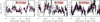 |
Fig. 2. Azimuth-velocity dispersion diagrams of atomic gas at selected radii in M 33. Each point corresponds to an individual measurement, i.e., the dispersion of each pixel within the map. Solid lines represent the results of a Fourier Transform model of the HI dispersion map (Sect. 3, assuming a cold neutral medium case). The dispersions are from the VLA 100 pc resolution data. |
To investigate the properties of the asymmetric random motions of the atomic gas, we expanded the isotropic random motions σiso of Eq. (2) with Fourier coefficients, following σiso, asym = ∑kσkcosk(ϕ − ϕk), where k is an integer. The isotropic axisymmetric component is σ0 and σk and ϕk are the amplitude and phase of the asymmetric modes in the velocity dispersion map. Both least-squares (LSQ) fits and discrete fast Fourier transforms (FFTs) were performed at the radial rings defined in Sect. 2 to cross-validate the analysis. The minor differences between fits and FFTs are that fits provide formal errors for the phases and amplitudes, and are more time consuming than FFTs. To avoid possible degeneracies, divergence, and increased computational time during minimizations, the maximum order that was fit is k = 4 (harmonics of k = 2). This maximum order is much smaller than the last order yielded by FFTs, which is the number of points in the azimuthal dimension at a given radius. The instrumental and thermal contributions were subtracted from the original maps before derivations of the kinematic harmonics.
Figure 3 shows the results of the FFT derivation for the 100 pc resolution VLA observation in the CNM case, with the amplitudes (top panel) and phases (middle panel) of the first four Fourier modes. The comparison of the bisymmetric amplitude with the first-, third-, and fourth-order terms is shown in the bottom panel of Fig. 3. Results of the LSQ fits are not shown because they are extremely similar to the FFTs.
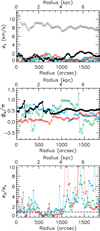 |
Fig. 3. Results of the discrete FFT of the HI velocity dispersion map of M 33 (100 pc resolution, in the CNM case). The amplitudes (upper panel) and phases (middle panel) of the Fourier modes are shown as black open circles (k = 0), green open circles (k = 1), filled circles (k = 2), blue upward filled triangles (k = 3), and red open diamonds (k = 4). The reference ϕ = 0 is chosen along the semi-major axis of the NE approaching half of M 33. Bottom panel: σ2/σk, using the same colors and symbols as above for the k = 1, 3, 4 modes. The range of ratios is chosen up to 10 for clarity, but the total range is 78 for σ2/σ1 and σ2/σ4, and 12 for σ2/σ3. |
The amplitude of the axisymmetric term is unsurprisingly similar to the azimuthally averaged velocity dispersion. The other modes are weak, with median amplitudes of σ1 = 0.6 km s−1, σ2 = 1.2 km s−1, σ3 = 0.6 km s−1, and σ4 = 0.7 km s−1. The bisymmetry is the most interesting mode. It shows the largest variation, which can reach 25% of the axisymmetric value at around R = 1500″ (6 kpc). It is stronger than σ1, σ3, and σ4 in ∼80%, 80%, and 65% of the cases, respectively. In the inner region (R < 1000″, or 4 kpc), these ratios fall to 65% for the k = 1 and k = 3 amplitudes, and to 40% for k = 4. We can thus define the locations where the bisymmetry is not stronger than other asymmetries as the locations where σ2 is weaker than at least two other modes, that is 188″ ≤ R ≤ 237″, 513″ ≤ R ≤ 687″, and 737″ ≤ R ≤ 837″. These regions are highlighted in subsequent figures. In the outer region (R > 1000″) it significantly dominates the other modes, by factors of 5, 4, and 7 on average (respectively to the k = 1, 3, 4 modes), reaching up to 78 times the k = 1 and k = 4 terms, and 12 times the k = 3 term.
The phases of the asymmetries contain a wealth of information as well. They show extended angular ranges where they remain closer or aligned with one of the principal axes of the M 33 disk, modulo half or one period of each mode. In other words, ϕ1 is consistent with the position of the minor and major axes (2.4 < R < 3.4 kpc, 4 < R < 5 kpc, R > 6 kpc) with some variation elsewhere, ϕ2 is mostly aligned with the minor axis, except for R = 0.7 and 1.5−2.5 kpc, ϕ3 remains close to 2π/3 in the inner disk half and to π/3 beyond R = 5.2 kpc (the period and half-period of the k = 3 mode, respectively), while ϕ4 shows three steps, one close to the major axis for R < 3 kpc (ϕ4 ∼ 0), one with the half-period of the k = 4 mode for 3 < R < 5.5 kpc (ϕ4 ∼ π/4) and another close to π/3 beyond 5.5 kpc. In the azimuth-dispersion diagrams drawn at selected radial rings of 0.2 kpc in width (Fig. 2), the solid lines show the results of the FFT models, highlighting the effects of the bisymmetry (all panels), the k = 1 mode (R = 3 kpc, middle panel), and the k = 4 mode (R = 1.5 kpc, left panel).
Finally, comparable results have been obtained with the 70 pc and 490 pc data. We also performed the same analysis in the WNM case for the 100 pc resolution data. The phases are comparable to the CNM case, but on average σ0 drops by 25%, while the median σ1, σ2, σ3, and σ4 rises respectively by a factor of 1.2, 1.1, 1.4, and 1.6, though it remains small. The k = 2 mode thus still dominates the asymmetric random motions in the WNM case.
4. Velocity anisotropy of gas in M 33
We now consider that gas can behave like a collisionless medium. The axisymmetric and anisotropic velocity model of Eq. (1) can be recast in
The expression with cos2ϕ therefore implies that such an anisotropic velocity dispersion model looks like a bisymmetric mode that has a null phase, i.e., aligned with the major or minor axis (depending on the sign of  ). The significant bisymmetric perturbation mostly aligned with the minor axis found in the HI velocity dispersion map of M 33 could thus be interpreted as a signature of velocity anisotropy, except maybe for the clearly identified regions of weaker k = 2 mode (see Sect. 3). The anisotropic velocity model makes it possible to constrain the two planar components and study the structure of orbits of gas in M 33 through the azimuthal anisotropy parameter βϕ. We also apply this model to observations of the molecular gas (Sect. 4.2).
Non-linear LSQ fits of Eq. (1) to σlos were performed using the program developed in Chemin (2018) for stellar disks. It fits radial, tangential, and vertical components of the random motion ellipsoid to a vector of observed dispersions at a given radius. A more developed model where the anisotropic dispersion components are asymmetric should also be considered to allow direct comparisons with Sect. 3. Yet such modeling is beyond the scope of the article. We refer to Chemin (2018) for more details of the minimization process and the validation of the methodology.
As σR, σϕ, and σz are expected to be roughly comparable, degeneracies can occur if the model is fit blindly to the observations. To make the analysis possible, we chose to hold the vertical component constant and let the radial and tangential dispersions vary freely. The value of σz can then be varied to measure its effect on the values of σR and σϕ. Fits with σz assumed constant as a function of R were performed, as well as others where σz varied with radius. In this latter case, it was fixed at the azimuthally averaged dispersion ⟨σlos⟩ϕ (dashed lines in Figs. 4, 5, and 9). In the case when σz was assumed constant, iterations in the range 4 ≤ σz ≤ 10 km s−1 were made for the atomic gas, sampled every 0.2 km s−1. This broad range of values contains the line-of-sight dispersion of ∼8 km s−1 observed in nearly face-on HI disks (Shostak & van der Kruit 1984; van der Kruit & Shostak 1984), and which is a good proxy for σz. For the molecular gas, we explored 2 ≤ σz ≤ 5 km s−1 because the velocity dispersions are lower. The resulting anisotropy parameters are not observed to be strongly dependent on the choice of σz (see also Chemin 2018). We define the quoted error on σR and σϕ at a given value of σz and at a given radius as the standard deviation of the posterior distribution of the parameters, and that for βϕ as the propagation of the σR and σϕ uncertainties.
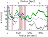 |
Fig. 4. Results of the anisotropic and axisymmetric velocity model for the atomic gas in Messier 33 (100 pc resolution data). Results are those of the one-parameter model and show the profile of σR (σϕ, respectively) as filled green circles (open diamonds), obtained assuming σϕ = σz = ⟨σlos⟩ϕ (σR = σz = ⟨σlos⟩ϕ). A dashed blue line is for ⟨σlos⟩ϕ (corrected from instrumental dispersion). Results obtained assuming a null thermal component. The shaded areas highlight the regions where the k = 2 mode was found to be weaker than other dispersion asymmetries (see Sect. 3). |
4.1. Results for the atomic neutral hydrogen
4.1.1. One-parameter model
A first goal is to assess whether isotropy is present within the model of Eq. (1). In this context, we tried to maximize the likelihood of finding isotropy by fixing σR = σz = ⟨σlos⟩ϕ, with σϕ as the only free parameter, and alternatively σϕ = σz = ⟨σlos⟩ϕ with σR as free parameter. We would indeed expect σϕ ≃ ⟨σlos⟩ϕ and σR ≃ ⟨σlos⟩ϕ, respectively, in those particular cases. The result is displayed in Fig. 4 (for the CNM case). The locations where σR or σϕ is closer to ⟨σlos⟩ϕ are R ∼ 1 kpc, and 2 ≤ R ≲ 3.5 kpc. These radii match closely those where the bisymmetry was found dominated by other asymmetries (Sect. 3). The radial (azimuthal) component is observed to be larger (smaller, respectively) than ⟨σlos⟩ϕ in most disk regions. Beyond 4 kpc, the difference with ⟨σlos⟩ϕ is important, up to 2 and 3 km s−1 for σR and σϕ (respectively), which is significant compared to the formal errors of the fits (≪1 km s−1). Comparisons between the two isotropic fits show that the model at free σR is significantly worse than the one at free σϕ, particularly in the outer disk. Indeed the assumption σϕ = ⟨σlos⟩ϕ automatically maximizes the tangential component, and in regions where the velocity dispersion map exhibits larger values near the minor axis, the model has no other choice than finding an even larger radial component than ⟨σlos⟩ϕ, hence yielding a best-fit σlos model that overestimates the bulk of the observed σlos. We also performed fits with σT = 6 km s−1 (not shown), but they failed in more than 75% of the rings. Results for a one-parameter case that most closely approaches an axisymmetric and isotropic model thus confirm the results found in Sect. 3: axisymmetry with isotropy cannot apply to the HI random velocity field of M 33.
4.1.2. Two-parameter model
Figure 5 shows the results found for σR and σϕ for the VLA 100 pc resolution map, assuming a null thermal component. The results corresponding to the warm neutral medium case are briefly discussed below. Results for σz = ⟨σlos⟩ϕ only are shown for clarity. Beyond R = 2 kpc, the azimuthal dispersion decreases by ∼6 km s−1, while the radial dispersion tends to increase slightly, although bumps are observed. In the inner kiloparsec, the overall variation of σR reaches ∼5 km s−1. For the most realistic σz values (σz < 10 km s−1) the results yield 0.5 ≤ σz/σR ≤ 0.9.
The resulting anisotropy parameter in the disk mid-plane is shown in Fig. 6 for the three resolutions of the HI data, again for σz = ⟨σlos⟩ϕ (solid lines). The result for another value, σz = 4 km s−1, for the 70 pc resolution data is also given (dotted line). It shows that the impact on βϕ of the choice of σz is negligible as differences in anisotropy parameter ≲0.15 are observed. A similar finding with stellar velocity anisotropy was presented in Chemin (2018).
The anisotropy parameters of the VLA 70 and 100 pc resolution H I data match perfectly. In the inner R = 3.5 kpc, βϕ is highly variable, sometimes corresponding to isotropic-to-radial motions (≲0.25), sometimes more radially biased (∼0.4), or showing dips down to −0.4 (R ∼ 0.7 and 2.2 kpc). Beyond R = 3.5 kpc, βϕ increases steadily reaching ∼0.8, showing that orbits become more radial at large radii.
The radially oriented orbits at large radius are also observed in the 490 pc resolution DRAO data (bottom panel of Fig. 6). The variations occurring on small angular scales are lost, however, because of the lower resolution. The dip of βϕ at R ∼ 0.7 kpc is not observed, while the second dip seems to be detected at ∼2.5 kpc, although at a lower (absolute) amplitude than at higher resolution, making the velocity ellipsoid more consistent with isotropy. Given the coincidence of the dips within or close to the regions where σ2 was measured lower, we interpret such negative values as a failure of the anisotropic velocity model at these locations.
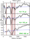 |
Fig. 6. Profiles of azimuthal velocity anisotropy βϕ of the atomic gas in M 33 at different angular resolutions. Solid lines show the anisotropy profiles obtained assuming σz = ⟨σlos⟩ϕ and a null thermal component. Short-dashed lines show the ±1 rms errors; a dotted line is an illustration of result choosing another vertical dispersion, σz = 4 km s−1 (70 pc resolution only); and a blue long-dashed line is the velocity anisotropy profile expected from the epicycle theory (Sect. 5). Shaded areas are as in Fig. 4. |
The effects of isotropic and radial orbits on σlos are shown in azimuth-dispersion diagrams of Fig. 7 (solid lines), as extracted from the 70 pc and 490 pc resolution HI observations. The widths of the radial rings were set to 0.1−0.2 kpc for the 70 pc resolution and 0.3−0.5 kpc for the 490 pc resolution. The left column illustrates locations where the anisotropic models found isotropy, the middle column is for gas orbits that are found more radial, and the right column illustrates one of the locations of a hypothetical tangentially biased orbit in the VLA data. While the model dispersion clearly varies with ϕ on a large angular scale, it does not account for the variations seen on smaller scales.
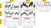 |
Fig. 7. Same as Fig. 2, but using HI data from VLA (70 pc resolution), DRAO (490 pc resolution), and CO data from IRAM 30 m antenna (50 pc resolution) to show results of the anisotropic velocity dispersion model (Sect. 4). The columns illustrate various cases of velocity anisotropy parameter found by the best-fit model: βϕ ∼ 0 (for isotropy, left ), 0 < βϕ (for radial bias, middle), βϕ < 0 (for supposedly tangential bias, right). For each resolution, the selected radii are among the best positions illustrating each case of anisotropy parameter, following Fig. 6. Solid lines represent the best-fit dispersion model at the considered radii, assuming σz = ⟨σlos⟩ϕ. |
As for the case of HI seen as a warm neutral medium (σT = 6 km s−1), βϕ is shown in Fig. 8, again assuming σz = ⟨σlos⟩ϕ. The anisotropy could not be derived for the outer disk because there is little room left for both planar components. This shows that at least some of the HI is cool in the outer region within the anisotropy assumption. The remaining velocity anisotropy is stronger than in the case σT = 0 km s−1, corresponding to even more radially biased gas orbits.
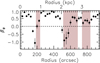 |
Fig. 8. Profile of azimuthal anisotropy βϕ of the velocity dispersion of the atomic gas in M 33 obtained using the 100 pc resolution VLA data by assuming σz = ⟨σlos⟩ϕ and HI as a warm neutral medium (thermal component of 6 km s−1). Shaded areas are as in Fig. 4. |
4.2. Results for the molecular gas
Results of the two-parameter model for the molecular gas, derived from the CO data, are shown in Fig. 9, obtained assuming σz = ⟨σlos⟩ϕ. Examples of azimuth-dispersion diagrams with the σlos models are shown in Fig. 7 (ring of 0.35 kpc in width). Similarly to the atomic gas, the variation of the molecular gas velocity anisotropy as a function of σz is negligible within the spanned range of σz. The velocity anisotropy parameter is highly scattered (⟨βϕ⟩∼0, on average, throughout the disk).
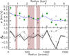 |
Fig. 9. Results for the molecular gas in Messier 33. Top: profiles of σR and σϕ of CO gas, obtained assuming σz = ⟨σlos⟩ϕ (dashed blue line, corrected for instrumental dispersion) and a null thermal component. Filled circles are for σR and open diamonds are for σϕ. Bottom: profiles of azimuthal velocity anisotropy βϕ of CO gas. The solid line shows the anisotropy obtained assuming σz = ⟨σlos⟩ϕ and a null thermal component, and dashed lines show the ±1 rms errors. For comparison, the anisotropy of the atomic gas as derived from all pixels in the 100 pc resolution velocity dispersion map is shown as a dotted line, and that derived using only the pixels at the positions of the molecular clouds as open triangles. Filled circles are values derived by masking a few deviant dispersions of CO clouds (σlos > 5 km s−1). Shaded areas are as in Fig. 4. |
We inspected the origin of the significant βϕ troughs at R = 1.7, 4.6, and 5.1 kpc and found they are caused by the presence of a few deviant observed dispersions, namely σlos ∼ 6.2 km s−1 along ϕ = 0 (R = 1.7 kpc), σlos ∼ 7.2 km s−1 along ϕ = 0 (R = 4.6 kpc), or σlos ∼ 6.4 km s−1 along ϕ = π (R = 5.1 kpc), while at these radii the other points are almost exclusively below 4.5 km s−1. The masking of such outlying points made the anisotropy parameter closer to 0 (filled circles in Fig. 9). A close inspection of σlos at R = 5.1 kpc shows no clear sine pattern that could yield βϕ < 0. Therefore, as for the HI, there is no evidence of a strong tangential bias of velocity anisotropy in the molecular gas in M 33.
The CO velocity anisotropy parameter is roughly in agreement with that of the atomic gas (dotted line) in the inner region, with the exception of R = 1.7 kpc. Interestingly, at larger radius where the HI velocity dispersion has become strongly anisotropic, the orbital structure of CO and HI in the mid-plane differ fundamentally. To verify whether these differences may be artifacts, we measured the velocity anisotropy of the atomic gas in a comparable way to that of the CO gas. This was done by using only the HI velocity dispersions at the locations of the discrete molecular clouds, instead of the whole HI dispersion map. The result shown as open triangles in Fig. 9 indicates that this HI anisotropy profile perfectly agrees with the profile inferred using the whole velocity dispersion field, including the outer regions with stronger HI radial bias. This suggests that the sparser distribution of points in the disk for the molecular gas than for the atomic gas is not the cause of the molecular-atomic difference.
In summary, we find no compelling evidence for a velocity ellipsoid of the molecular clouds being aligned systematically towards (or perpendicular to) the direction of the galactic centre of M 33. This result may indicate that the dynamics of clouds is locally dominated by the cloud gravitational potential. It also highlights the need for velocity dispersion maps of molecular gas in galaxies rather than cloud-based measurements to make the comparison with the HI gas more appropriate.
5. Discussion
This work is the first to our knowledge that examines the effects of the collisionless medium hypothesis for gas on the structure of velocity dispersions, and the implied azimuthal-to-radial axis ratio of the velocity ellipsoid in galactic disks. Therefore, no fully appropriate comparisons with other observational studies of the gas component are available.
Comparisons can be made with the stellar collisionless kinematic tracer, however. Observations of radially biased stellar random motions is not rare among nearby spiral galaxies. Taking the example of our Galaxy, the velocity anisotropy of stars in the disk of the Milky Way derived by Chemin (2018) using stellar dispersions from the Second Gaia Data Release published in Gaia Collaboration (2018) shows quite similar values to the atomic gas of M 33 inside R = 4 kpc, as well as the increase towards large radii. A possible mechanism for the origin of stellar anisotropic orbits in the Galaxy may be radial migration induced by the dynamics of spiral arms (Roškar et al. 2012; Grand et al. 2014). The similarity of the velocity anisotropy of HI gas in M 33 to that of the stars in the Milky Way may provide clues for the interpretation of the results presented here. There are clear spiral-like structures at large radius in M 33 (Fig. 1), with location and shape correlated with the bisymmetry in the velocity dispersion. Although non-axisymmetric perturbations are not necessary to have an anisotropic velocity dispersion ellipsoid, we can speculate that the spiral arms in M 33 could enhance the velocity anisotropy parameter in the outer disk regions if part of the HI gas in M 33 behaves like a collisionless medium. We also note that disks of similar stellar mass to that of M 33 show −0.1 ≲ βϕ ≲ 0.2 (Chemin 2018), thus stellar orbits in these galaxies are more isotropic.
The analysis also shows that it is not possible to strongly constrain σz given the small scatter of βϕ as a function of σz. It is nevertheless worth mentioning that under realistic hypotheses on σz, the range of σz/σR found for gas in M 33 is consistent with the value of ∼0.65 found for late-type stellar disks by Pinna et al. (2018).
Comparisons can be made with numerical simulations as well. Hydrodynamical modeling of gas in simulated spiral galaxies shows velocity dispersion components that are anisotropic (Bottema 2003; Agertz et al. 2009). In these numerical models, the tangential component is smaller than the radial dispersion. This is in agreement with most of our measurements. The simulations of Agertz et al. (2009) are interesting for our study because they are supposed to simulate a disk with similar physical properties to M 33. They showed that the planar dispersion, σP, given by the root mean squared value of σR and σϕ, is twice larger than σz. If we restrict the comparison to the radial range 4−7.5 kpc where M 33 shows a more significant anisotropy parameter in the framework of an axisymmetric and anisotropic velocity model, the simulations of Agertz et al. (2009) show σz within 3.5−7 km s−1 once the spiral-like features are well defined in the simulated density map. Our models show that σP ∼ 2σz in M 33 for σz ∼ 6 km s−1. Therefore, comparable planar and vertical dispersions are found in both the observations and simulations. More broadly, within the range of vertical dispersions that has been investigated here, we find σP from ∼10 km s−1 (σz = 10 km s−1) to ∼13 km s−1 (σz = 4 km s−1), hence σP/σz from ∼0.9−1 to ∼3−3.2, respectively. The vertical motion is thus the main driver of the ratio. For σz = ⟨σlos⟩ϕ (∼8 km s−1), σP/σz ∼1.4−1.5, which is close to the value expected for an isotropic velocity ellipsoid ( ).
).
Agertz et al. (2009) then found that σϕ/σR is roughly consistent with the expectation of the epicyclic approximation (EA) which considers collisionless orbits that only slightly deviate from circularity. The EA stipulates that σϕ/σR is related to the slope of the circular velocity vc (e.g., Binney & Tremaine 2008):
The epicycle anisotropy of M 33,  is shown as a dashed blue line in Fig. 6. It was derived using the model of the HI rotation curve of M 33 by Koch et al. (2018) as a proxy for the circular velocity. The assumption that the circular velocity can be approximated by the tangential velocity is reasonable for gas, except maybe in lower mass disks (Dalcanton & Stilp 2010). The value of βEA shows very little variation as a function of radius. Interestingly, the inner R = 4 kpc of M 33 is the range of radii where the anisotropy is mild (Fig. 6) and differs by ≲0.25 from that derived from the epicyclic approximation (except for the two outlying dips at R ∼ 0.7 and 2.1 kpc). The velocity anisotropy of gas is systematically larger than expected from the epicyclic approximation beyond R ∼ 5 kpc, however. Equation (4) cannot allow the observed strongly radial HI orbits because the rotation curve of M 33 is barely rising at these radii (βEA ∼ 0.4). We would need a decreasing rotation curve to get βEA > 0.5 compatible with the observed velocity anisotropy in the plane. Our results thus do not fully agree with those found with the numerical simulations of Agertz et al. (2009) in the disk regions of stronger radial bias. On the other hand, if the ellipsoid of velocity is isotropic, then the epicyclic approximation is violated as well because a linearly rising velocity curve with radius is strictly required for an EA–isotropy agreement. This indicates a failure of the epicycle approximation of orbits for the gas component. Interestingly, this discrepancy is reminiscent of the result found in Chemin (2018) for stellar disks where the diversity of stellar orbits could not be reproduced by the theory.
Is the HI velocity dispersion ellipsoid of Messier 33 anisotropic or isotropic? Choosing a side for this question is not an easy task as the two models both explain the major asymmetry. The Fourier analysis has the flexibility to probe a large number of modes, hence isotropic and asymmetric models are unsurprisingly more accurate in modeling σlos. An intriguing result of this work is the observation that the orientation of kinematic perturbations are often aligned with the principal disk axes (modulo half and full periods) as if a projection effect affected significantly the velocity dispersion map of M 33. Such coincidences may be fortuitous in M 33 given that asymmetries in the gas density often appear coincident with the dispersion asymmetries (Fig. 1). This also suggests that further analyses of phases of asymmetric modes inside velocity dispersion maps are promising to assess the nature of gaseous velocity ellipsoids. If the phase angles were found systematically near the principal axes, at the positions of supposedly stronger velocity anisotropy, then it would rule out isotropic velocity ellipsoids since that occurrence should occur only rarely for a random distribution of phase angles of perturbations in the isotropic scenario. Data from deep surveys like THINGS (Walter et al. 2008), HALOGAS (Heald et al. 2011), and LittleTHINGS (Hunter et al. 2012) for the neutral atomic gas, or PHANGS-ALMA (Sun et al. 2018) for the molecular gas will be helpful to study that problem.
6. Summary
Messier 33 has a non-axisymmetric distribution of observed random motions of HI gas. There is a prominent pattern that makes the HI velocity dispersion weaker near the major axis and stronger near the minor axis of the galaxy. The velocity dispersion of the R > 4 kpc disk can locally be larger by up to 60% than the azimuthally averaged value. Hypotheses allying axisymmetry and isotropy are ruled out to explain the variations of the velocity dispersion.
Among the models presented in this study a Fourier transform has shown that bisymmetric random motions having an amplitude of up to 2 km s−1 (25% of the axisymmetric value) must be invoked to explain the discrepancy while maintaining isotropy. It dominates the harmonic asymmetries in the random motions, and first-, third-, and fourth-order motions were found mostly weaker. The phase angles of the asymmetries are often seen close to the principal axes of the HI disk, and particularly the bisymmetry, which is aligned with the minor axis. The asymmetries coincide well with the non-axisymmetric spiral-like distribution of HI gas in M 33.
Another model was to consider that the velocity dispersion ellipsoid is axisymmetric but anisotropic, acting as if part of gas behaved like a collisionless medium. That led us to constrain the radial and tangential components of the ellipsoid (σR and σϕ) at fixed vertical dispersion σz, and from which the azimuthal velocity anisotropy parameter βϕ = 1 − (σϕ/σR)2 could be measured. In the framework of this axisymmetric model, βϕ is mostly positive and maximum at R ∼ 6 kpc, indicating orbits of the atomic gas that are strongly radial. The perturbed dynamics in the spiral-like structure could be responsible for the velocity anisotropy. It was also found that while anisotropic velocity dispersions could be measured when the HI gas is treated like a CNM, it is not the case in the outer regions of stronger velocity anisotropy when the gas is seen as a WNM. A high thermal component does not leaves as much room for the planar motions.
As for the CO gas traced by a collection of a few hundreds of molecular clouds, βϕ is highly scattered and did not allow us to draw firm conclusions about the shape of CO cloud orbits. Although the comparison with HI gas remains limited because cloud-based dispersions were used in this analysis, unlike HI dispersions this result is not surprising if velocity dispersions of molecular clouds are driven by local cloud dynamics.
These results were found only marginally dependent on the assumptions made for σz (chosen as representative of values observed in face-on nearby disks). In future works, we will pursue the analysis of the properties of asymmetries in gas velocity dispersions by means of a larger sample of disk galaxies via further sensitive HI and CO measurements, and investigate to what extent anisotropic velocity ellipsoids can still explain the asymmetric gas random motions.
Acknowledgments
We are very grateful to an anonymous referee for insightful propositions which improved the analysis and the content of the article. This research was supported by the Comité Mixto ESO-Chile and the DGI at University of Antofagasta, and J. Braine by the MINEDUC-UA project code ANT 1755.
References
- Agertz, O., Lake, G., Teyssier, R., et al. 2009, MNRAS, 392, 294 [NASA ADS] [CrossRef] [Google Scholar]
- Bacchini, C., Fraternali, F., Iorio, G., & Pezzulli, G. 2019, A&A, 622, A64 [NASA ADS] [CrossRef] [EDP Sciences] [Google Scholar]
- Bershady, M. A., Verheijen, M. A. W., Swaters, R. A., et al. 2010, ApJ, 716, 198 [NASA ADS] [CrossRef] [Google Scholar]
- Binney, J., & Tremaine, S. 2008, Galactic Dynamics: Second Edition (Princeton: Princeton University Press) [Google Scholar]
- Bottema, R. 2003, MNRAS, 344, 358 [NASA ADS] [CrossRef] [Google Scholar]
- Braine, J., Rosolowsky, E., Gratier, P., Corbelli, E., & Schuster, K.-F. 2018, A&A, 612, A51 [NASA ADS] [CrossRef] [EDP Sciences] [Google Scholar]
- Chemin, L. 2018, A&A, 618, A121 [CrossRef] [EDP Sciences] [Google Scholar]
- Combes, F., & Becquaert, J.-F. 1997, A&A, 326, 554 [NASA ADS] [Google Scholar]
- Corbelli, E., & Schneider, S. E. 1997, ApJ, 479, 244 [NASA ADS] [CrossRef] [Google Scholar]
- Corbelli, E., Thilker, D., Zibetti, S., Giovanardi, C., & Salucci, P. 2014, A&A, 572, A23 [NASA ADS] [CrossRef] [EDP Sciences] [Google Scholar]
- Corbelli, E., Braine, J., Bandiera, R., et al. 2017, A&A, 601, A146 [NASA ADS] [CrossRef] [EDP Sciences] [Google Scholar]
- Dalcanton, J. J., & Stilp, A. M. 2010, ApJ, 721, 547 [NASA ADS] [CrossRef] [Google Scholar]
- Draine, B. T. 2011, Physics of the Interstellar and Intergalactic Medium (Princeton: Princeton University Press) [Google Scholar]
- Druard, C., Braine, J., Schuster, K. F., et al. 2014, A&A, 567, A118 [NASA ADS] [CrossRef] [EDP Sciences] [Google Scholar]
- Epinat, B., Amram, P., Balkowski, C., & Marcelin, M. 2010, MNRAS, 401, 2113 [NASA ADS] [CrossRef] [Google Scholar]
- Fraternali, F., Oosterloo, T., Sancisi, R., & van Moorsel, G. 2001, ApJ, 562, L47 [NASA ADS] [CrossRef] [Google Scholar]
- Fraternali, F., van Moorsel, G., Sancisi, R., & Oosterloo, T. 2002, AJ, 123, 3124 [NASA ADS] [CrossRef] [Google Scholar]
- Gaia Collaboration (Katz, D., et al.) 2018, A&A, 616, A11 [NASA ADS] [CrossRef] [EDP Sciences] [Google Scholar]
- Grand, R. J. J., Kawata, D., & Cropper, M. 2014, MNRAS, 439, 623 [NASA ADS] [CrossRef] [Google Scholar]
- Gratier, P., Braine, J., Rodriguez-Fernandez, N. J., et al. 2010, A&A, 522, A3 [NASA ADS] [CrossRef] [EDP Sciences] [Google Scholar]
- Heald, G., Józsa, G., Serra, P., et al. 2011, A&A, 526, A118 [NASA ADS] [CrossRef] [EDP Sciences] [Google Scholar]
- Hunter, D. A., Ficut-Vicas, D., Ashley, T., et al. 2012, AJ, 144, 134 [NASA ADS] [CrossRef] [Google Scholar]
- Kalnajs, A. J. 1973, PASA, 2, 174 [Google Scholar]
- Kam, S. Z., Carignan, C., Chemin, L., et al. 2017, AJ, 154, 41 [NASA ADS] [CrossRef] [Google Scholar]
- Koch, E. W., Rosolowsky, E. W., Lockman, F. J., et al. 2018, MNRAS, 479, 2505 [CrossRef] [Google Scholar]
- Koyama, H., & Ostriker, E. C. 2009, ApJ, 693, 1346 [NASA ADS] [CrossRef] [Google Scholar]
- Martinsson, T. P. K., Verheijen, M. A. W., Westfall, K. B., et al. 2013, A&A, 557, A131 [NASA ADS] [CrossRef] [EDP Sciences] [Google Scholar]
- Oh, S.-H., Hunter, D. A., Brinks, E., et al. 2015, AJ, 149, 180 [NASA ADS] [CrossRef] [Google Scholar]
- Pinna, F., Falcón-Barroso, J., Martig, M., et al. 2018, MNRAS, 475, 2697 [NASA ADS] [CrossRef] [Google Scholar]
- Rosolowsky, E., & Leroy, A. 2006, PASP, 118, 590 [NASA ADS] [CrossRef] [Google Scholar]
- Roškar, R., Debattista, V. P., Quinn, T. R., & Wadsley, J. 2012, MNRAS, 426, 2089 [NASA ADS] [CrossRef] [Google Scholar]
- Shostak, G. S., & van der Kruit, P. C. 1984, A&A, 132, 20 [NASA ADS] [Google Scholar]
- Sun, J., Leroy, A. K., Schruba, A., et al. 2018, ApJ, 860, 172 [NASA ADS] [CrossRef] [Google Scholar]
- van der Kruit, P. C., & Shostak, G. S. 1984, A&A, 134, 258 [NASA ADS] [Google Scholar]
- Visser, H. C. D. 1980, A&A, 88, 149 [NASA ADS] [Google Scholar]
- Walter, F., Brinks, E., de Blok, W. J. G., et al. 2008, AJ, 136, 2563 [NASA ADS] [CrossRef] [Google Scholar]
All Figures
|
Fig. 1. Observational data of Messier 33. Left panel: HI column density map (VLA, 100 pc resolution, logarithmic stretch) with Spitzer/IRAC 3.6 μm stellar distribution overlaid (gray contours, showing the 0.1, 0.3, 0.5, 0.7, 0.9, 1.4, and 2.5 MJy sr−1 levels). Right panel: observed HI velocity dispersion (VLA, 100 pc resolution, not corrected for the instrumental dispersion), with HI column densities contours (1, 2, 3 × 1021 cm−2). The dashed line represents the location of the major axis of the inner unwarped disk, with position angle of 22.5°. Concentric ellipses show the projected locations of R = 2, 4, 6 kpc. |
| In the text | |
|
Fig. 2. Azimuth-velocity dispersion diagrams of atomic gas at selected radii in M 33. Each point corresponds to an individual measurement, i.e., the dispersion of each pixel within the map. Solid lines represent the results of a Fourier Transform model of the HI dispersion map (Sect. 3, assuming a cold neutral medium case). The dispersions are from the VLA 100 pc resolution data. |
| In the text | |
|
Fig. 3. Results of the discrete FFT of the HI velocity dispersion map of M 33 (100 pc resolution, in the CNM case). The amplitudes (upper panel) and phases (middle panel) of the Fourier modes are shown as black open circles (k = 0), green open circles (k = 1), filled circles (k = 2), blue upward filled triangles (k = 3), and red open diamonds (k = 4). The reference ϕ = 0 is chosen along the semi-major axis of the NE approaching half of M 33. Bottom panel: σ2/σk, using the same colors and symbols as above for the k = 1, 3, 4 modes. The range of ratios is chosen up to 10 for clarity, but the total range is 78 for σ2/σ1 and σ2/σ4, and 12 for σ2/σ3. |
| In the text | |
|
Fig. 4. Results of the anisotropic and axisymmetric velocity model for the atomic gas in Messier 33 (100 pc resolution data). Results are those of the one-parameter model and show the profile of σR (σϕ, respectively) as filled green circles (open diamonds), obtained assuming σϕ = σz = ⟨σlos⟩ϕ (σR = σz = ⟨σlos⟩ϕ). A dashed blue line is for ⟨σlos⟩ϕ (corrected from instrumental dispersion). Results obtained assuming a null thermal component. The shaded areas highlight the regions where the k = 2 mode was found to be weaker than other dispersion asymmetries (see Sect. 3). |
| In the text | |
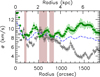 |
Fig. 5. Same as Fig. 4, but for the two-parameter model with σR and σϕ as free parameters. |
| In the text | |
|
Fig. 6. Profiles of azimuthal velocity anisotropy βϕ of the atomic gas in M 33 at different angular resolutions. Solid lines show the anisotropy profiles obtained assuming σz = ⟨σlos⟩ϕ and a null thermal component. Short-dashed lines show the ±1 rms errors; a dotted line is an illustration of result choosing another vertical dispersion, σz = 4 km s−1 (70 pc resolution only); and a blue long-dashed line is the velocity anisotropy profile expected from the epicycle theory (Sect. 5). Shaded areas are as in Fig. 4. |
| In the text | |
|
Fig. 7. Same as Fig. 2, but using HI data from VLA (70 pc resolution), DRAO (490 pc resolution), and CO data from IRAM 30 m antenna (50 pc resolution) to show results of the anisotropic velocity dispersion model (Sect. 4). The columns illustrate various cases of velocity anisotropy parameter found by the best-fit model: βϕ ∼ 0 (for isotropy, left ), 0 < βϕ (for radial bias, middle), βϕ < 0 (for supposedly tangential bias, right). For each resolution, the selected radii are among the best positions illustrating each case of anisotropy parameter, following Fig. 6. Solid lines represent the best-fit dispersion model at the considered radii, assuming σz = ⟨σlos⟩ϕ. |
| In the text | |
|
Fig. 8. Profile of azimuthal anisotropy βϕ of the velocity dispersion of the atomic gas in M 33 obtained using the 100 pc resolution VLA data by assuming σz = ⟨σlos⟩ϕ and HI as a warm neutral medium (thermal component of 6 km s−1). Shaded areas are as in Fig. 4. |
| In the text | |
|
Fig. 9. Results for the molecular gas in Messier 33. Top: profiles of σR and σϕ of CO gas, obtained assuming σz = ⟨σlos⟩ϕ (dashed blue line, corrected for instrumental dispersion) and a null thermal component. Filled circles are for σR and open diamonds are for σϕ. Bottom: profiles of azimuthal velocity anisotropy βϕ of CO gas. The solid line shows the anisotropy obtained assuming σz = ⟨σlos⟩ϕ and a null thermal component, and dashed lines show the ±1 rms errors. For comparison, the anisotropy of the atomic gas as derived from all pixels in the 100 pc resolution velocity dispersion map is shown as a dotted line, and that derived using only the pixels at the positions of the molecular clouds as open triangles. Filled circles are values derived by masking a few deviant dispersions of CO clouds (σlos > 5 km s−1). Shaded areas are as in Fig. 4. |
| In the text | |
Current usage metrics show cumulative count of Article Views (full-text article views including HTML views, PDF and ePub downloads, according to the available data) and Abstracts Views on Vision4Press platform.
Data correspond to usage on the plateform after 2015. The current usage metrics is available 48-96 hours after online publication and is updated daily on week days.
Initial download of the metrics may take a while.