| Issue |
A&A
Volume 638, June 2020
|
|
|---|---|---|
| Article Number | A68 | |
| Number of page(s) | 11 | |
| Section | The Sun and the Heliosphere | |
| DOI | https://doi.org/10.1051/0004-6361/202037613 | |
| Published online | 12 June 2020 | |
A statistical study of the long-term evolution of coronal hole properties as observed by SDO
1
University of Graz, Institute of Physics, Graz, Austria
e-mail: This email address is being protected from spambots. You need JavaScript enabled to view it.
2
Centre for Plasma Astrophysics, KU Leuven, Leuven, Belgium
3
University of Zagreb, Faculty of Geodesy, Hvar Observatory, Zagreb, Croatia
4
National Space Institute, DTU Space, Denmark
5
University of Zagreb, Faculty of Science, Department of Geophysics, Zagreb, Croatia
6
Kanzelhöhe Observatory for Solar and Environmental Research, University of Graz, Graz, Austria
Received:
29
January
2020
Accepted:
21
April
2020
Abstract
Context. Understanding the evolution of coronal holes is especially important when studying the high-speed solar wind streams that emanate from them. Slow- and high-speed stream interaction regions may deliver large amounts of energy into the Earth’s magnetosphere-ionosphere system, cause geomagnetic storms, and shape interplanetary space.
Aims. By statistically investigating the long-term evolution of well-observed coronal holes we aim to reveal processes that drive the observed changes in the coronal hole parameters. By analyzing 16 long-living coronal holes observed by the Solar Dynamic Observatory, we focus on coronal, morphological, and underlying photospheric magnetic field characteristics, and investigate the evolution of the associated high-speed streams.
Methods. We use the Collection of Analysis Tools for Coronal Holes to extract and analyze coronal holes using 193 Å EUV observations taken by the Atmospheric Imaging Assembly as well as line–of–sight magnetograms observed by the Helioseismic and Magnetic Imager. We derive changes in the coronal hole properties and look for correlations with coronal hole evolution. Further, we analyze the properties of the high–speed stream signatures near 1AU from OMNI data by manually extracting the peak bulk velocity of the solar wind plasma.
Results. We find that the area evolution of coronal holes shows a general trend of growing to a maximum followed by a decay. We did not find any correlation between the area evolution and the evolution of the signed magnetic flux or signed magnetic flux density enclosed in the projected coronal hole area. From this we conclude that the magnetic flux within the extracted coronal hole boundaries is not the main cause for its area evolution. We derive coronal hole area change rates (growth and decay) of (14.2 ± 15.0)×108 km2 per day showing a reasonable anti-correlation (ccPearson = −0.48) to the solar activity, approximated by the sunspot number. The change rates of the signed mean magnetic flux density (27.3 ± 32.2 mG day−1) and the signed magnetic flux (30.3 ± 31.5 1018 Mx day−1) were also found to be dependent on solar activity (ccPearson = 0.50 and ccPearson = 0.69 respectively) rather than on the individual coronal hole evolutions. Further we find that the relation between coronal hole area and high-speed stream peak velocity is valid for each coronal hole over its evolution, but we see significant variations in the slopes of the regression lines.
Key words: Sun: corona / Sun: evolution / Sun: activity / Sun: magnetic fields / solar-terrestrial relations / solar wind
© ESO 2020
1. Introduction
Coronal holes (CH) are stable, long-lived structures usually observed in the solar corona as regions of reduced emission in extreme ultraviolet (EUV) or X-ray. Coronal holes are characterized by an open magnetic field configuration along which ionized atoms and electrons are accelerated into interplanetary space, forming high speed solar wind streams (HSS; Krieger et al. 1973; Nolte et al. 1976; Cranmer 2009). The interaction of HSSs with the preceeding ambient slow solar wind forms stream interaction regions (SIRs) which can develop into co-rotating interaction regions (CIRs; Wilcox 1968; Tsurutani et al. 2006) if the CH persists over multiple rotations. These transient features are the main source of usually weak to medium geomagnetic storms at Earth (see, e.g., Alves et al. 2006; Verbanac et al. 2011a; Vršnak et al. 2017; Yermolaev et al. 2018; Richardson 2018). Since the Skylab era, recurrent geomagnetic effects of CIRs have been associated with large-scale coronal signatures, the CHs. Nolte et al. (1976) first found an empirical relationship between the CH area and the peak bulk velocity of the solar wind. The linear CH area–HSS speed relation is supported by many studies, although different slopes of the regression lines are found (e.g., Nolte et al. 1978a; Vršnak et al. 2007; Tokumaru et al. 2017; Heinemann et al. 2018a; Hofmeister et al. 2018).
The long-term evolution of recurrent CH structures and the associated HSSs has rarely been investigated. Most studies focus on a snap-shot of the CH during its lifetime in the form of a case study (e.g., Gibson et al. 1999; Gopalswamy et al. 1999; Zhang et al. 2007; Yang et al. 2009) or statistical studies that do not separate the evolution of individual CHs (e.g., Harvey et al. 1982; Lowder et al. 2017; Hofmeister et al. 2017; Heinemann et al. 2019). In the Skylab era, Bohlin (1977) and Bohlin & Sheeley (1978) proposed that the area and the mean magnetic flux density of a CH are dependent on its age and Nolte et al. (1978a,b) used X-ray observations to show that CHs primarily evolve by sudden, large-scale shifts in the position of the boundaries. A change in the underlying photospheric magnetic field is believed to influence the appearance of the CHs in the corona (Wang & Sheeley 1990; Gosling 1996). In a more recent study, Ikhsanov & Tavastsherna (2015) showed that there are two magnetic field systems (large-scale high-latitude and small-scale low-latitude magnetic field systems) that play major roles in the evolution of the solar magnetic cycle and whose effects can be seen in the appearance of CHs. Wang & Sheeley (1990) showed in their current-free coronal model, that the long-term evolution of CHs and the associated wind streams is related to flux emergence in active regions and the subsequent flux transport processes. Coronal holes themselves seem to form in response to local (low-latitudes) or global (polar, high-latitudes) changes in the magnetic field topology. At low-latitudes, small-scale magnetic systems may manifest themselves as localized CHs that are the result of decaying local sunspot groups (Petrie & Haislmaier 2013) or are generated by other mechanisms that enable to “open” the magnetic field, such as coronal mass ejections (CMEs)/filament eruptions, flux accumulation, or flux emergence (e.g., Webb et al. 1978; Heinemann et al. 2018b). Heinemann et al. (2018a,b) provide an in-depth view of the evolution of one particular CH in 2012 from which they identified a clear evolutionary pattern in combination with a correlation to the underlying magnetic field.
To statistically obtain the evolutionary aspects of individual CHs in the photosphere and corona the current study investigates the evolution of 16 long-lived individual CHs in detail. The observational CH data cover most of the Solar Dynamics Observatory (SDO; Pesnell et al. 2012) era so far, starting from September 2010 until April 2019. This enables us to obtain a more general insight into the evolutionary processes of CHs by analyzing coronal and magnetic properties as well as the rates at which they change. Additionally, we investigate how changes in the observed CH on-disk characteristics affect the in-situ measured HSS parameters near Earth, and check whether or not the well-established CH area–HSS peak velocity relation holds over individual CH evolutions. For this we used data from the Global Geospace Science Wind satellite (Acuña et al. 1995) and the Advanced Composition Explorer (ACE; Stone et al. 1998).
2. Methods
2.1. Dataset
For this study, we focus on the long-term evolution of CHs and its properties. In order to derive significant correlations or trends, we properly chose the dataset applying the following constraints:
– We aim to analyze not only the intensity and morphological parameters of the CH evolution but also the change in the underlying photospheric magnetic field and enclosed magnetic flux. We are therefore limited to observations for which remote sensing magnetic field data are available. For this reason, data from the Atmospheric Imaging Assembly (AIA; Lemen et al. 2012) and the Helioseismic and Magnetic Imager (HMI; Schou et al. 2012; Couvidat et al. 2016) on board SDO were chosen for the analysis. SDO was preferred over the Solar and Heliospheric Observatory (SOHO; Domingo et al. 1995) due to the significantly lower noise in the line-of-sight (LoS) magnetograms of HMI, which is very relevant for regions of low magnetic field strength such as CHs.
– To analyze the long-term evolution of CHs, only CHs that showed a clear coronal signature for at least five consecutive solar disk passages were considered.
– The last condition was that the CH did not originate as or from a polar CH. This was considered due to high uncertainties in determining the CH area in polar regions due to projection and line–of–sight effects. Additionally the magnetic field observations of these areas are highly unreliable.
By considering the stated constraints, we extracted 16 CHs fulfilling those requirements over most of the operational life-time of SDO from 2010 to 2019.
2.2. Coronal hole detection and extraction
To identify and extract CHs we use the 193 Å filter of the AIA instrument onboard SDO as CHs can be well observed in the emission of highly ionized iron (especially Fe XII: 193/195 Å). The high contrast with the surrounding quiet Sun enables a good extraction of boundaries. To capture the long-term evolution, we extract each CH and its characteristics at each solar disk passage near the central meridian. Heinemann et al. (2018a,b) showed in a case study that one data point per rotation depicts the evolutionary trend sufficiently. We use the Collection of Analysis Tools for Coronal Holes (CATCH; Heinemann et al. 2019). CATCH uses a supervised threshold-based extraction that is modulated by the intensity gradient perpendicular to the CH boundary. For illustrative purposes we show in the right panel of Fig. 1 the extraction of a CH from May 29, 2013. In analogy to the right panel of Fig. 1, in Fig. A.1 we show a representative EUV image for every CH.
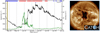 |
Fig. 1. Example of an in-situ signature of the solar wind data provided by the OMNI database (left), as a CH under study was observed near the center of the solar disk by SDO on May 29, 2013, at 18 UT (right). The black line shows the solar wind bulk velocity and green line represents the plasma density. The purple triangle represents the peak velocity and the horizontal bar the average interval to show the plateau speed. The colored bar on the top represents the in-situ polarity calculated after Neugebauer et al. (2002), with red being positive and blue negative polarity. Right panel: snapshot of the CH that is associated with this HSS, and the time of the SDO observation corresponds to the yellow vertical line in the left panel. The red line is the extracted CH boundary (using CATCH) and the yellow x represents the center of mass of the CH. |
The CHs were extracted from point spread function (PSF) deconvoluted, limb-brightening-corrected (Verbeeck et al. 2014) AIA 193 Å EUV images that were rebinned to a pixel resolution 1024 × 1024, corresponding to a plate scale of 2.4 arcsec per pixel. Reducing the size increases processing speed and has only negligible effects on the boundary extraction (e.g., see Heinemann et al. 2019). Furthermore, the boundaries were smoothed using morphological operators with a kernel of 2 × 2 pixel size.
To account for LoS, projection, and limb effects as well as for unreliable magnetograms near the poles, we only consider pixels at latitudes |λ|< 60° in our calculations, i.e. all pixels above 60° latitude were disregarded.
The properties of the photospheric magnetic field underlying the extracted CH boundary were derived from de-projected 720 s LoS HMI magnetograms which were chosen over its 45 s equivalent due to the lower photon noise of ≈3 Gauss near the disk center (Couvidat et al. 2016). The higher signal-to-noise ratio gives more reliable results for low magnetic field densities. The extracted CH boundaries were overlaid on the magnetograms to calculate the properties.
2.3. Coronal hole properties
All properties were derived using CATCH, which includes morphological properties like the CH area, shape, and position (center of mass), and properties of the underlying photospheric magnetic field like the signed mean magnetic flux density and magnetic flux. For more details about the extraction and calculation of the parameters and uncertainties, we refer to Heinemann et al. (2019) and references therein.
In this study we focus on the evolution of the primary parameters of the CH: the CH area (A), the signed mean magnetic flux density (Bs), and the signed magnetic flux (Φs). The signed magnetic flux density is a good indicator of the magnetic fine structure of a CH as it is directly correlated to the abundance and coverage of strong unipolar magnetic elements within CHs. It has been found that they are the main contributors to the signed CH flux (Hofmeister et al. 2019; Heinemann et al. 2019).
The average parameters over the evolution of a CH, denoted by an asterisk, are derived by calculating the mean over the evolution of a CH considering the uncertainties given by:
 (1)
(1)
 (2)
(2)
where Pi represents a CH property for every rotation (i) and σPi its uncertainty. The spread of the values over the whole evolution, σ*, is calculated by adding the mean uncertainty (first term) and the standard deviation of the mean (second term). The change rates of CH properties were calculated as follows:
 (3)
(3)
with P again representing a CH property (i.e., A, Bs, Φs) and t being the time of observation.
2.4. In-situ data
To make a more complete interpretation of the evolutionary effects of CHs on the in-situ measured signatures, we investigated the associated HSSs near 1 AU using five-minute plasma and magnetic field data provided by the OMNI1 database. OMNI in-situ measurements are propagated to the Earth’s bow shock nose.
HSSs signatures were classified using the criteria given by Jian et al. (2006, 2009) and cross-checked with ready HSS lists (maintained by S. Vennerstroem for 2010−2019). Identified HSS structures were associated to extracted CHs in two ways: first, by comparing the dominant polarity of the HSS (as given in Neugebauer et al. 2002) with the dominant polarity of the CH – small-scale turbulences (as reported in the Parker Solar Probe results by Bale et al. 2019) were neglected –; and second by considering the travel time of the HSS according to its speed (e.g., Vršnak et al. 2007). Time ranges covering ICME signatures were removed using ready-catalogs maintained by Richardson and Cane2 for ACE (see Richardson & Cane 2010, for a description of the catalog). Coronal holes that could not be associated with a HSS signature were excluded from the HSS analysis.
For each CH, we derive, if possible, the associated HSS speed peak and the plasma density and magnetic field at the same time, for each solar disk passage. From the peak, we define the plateau speed as the averaged peak speed of the HSS within an interval of [ − 2, +6] hours around the identified peak. The asymmetrical averaging interval was chosen to consider the asymmetry in the speed profile of HSSs and to avoid contribution from the stream interaction region. The plasma density and magnetic field magnitude for the identical time interval were also calculated in the same way.
Here, the aim was to verify whether or not and how the CH area–HSS speed relation (Nolte et al. 1976; Vršnak et al. 2007; Rotter et al. 2012; Tokumaru et al. 2017; Hofmeister et al. 2018) relates to the CH evolution. It has been found that there is a latitudinal dependence in CH area–HSS speed relation, and because we are interested in the CH area that affects Earth, that is, the geoeffective CH area, we correct for it. The geoeffective CH area can be calculated using the relation derived by Hofmeister et al. (2018):
 (4)
(4)
with φco being the latitudinal separation angle between the center of mass of the CH and the observing spacecraft. According to this statistical relation, there is no contribution to the HSS from CHs above a latitude of ≈60°, which seems to be valid in a first-order approximation (Vršnak et al. 2007). Consequently, we consider CH areas below 60°.
2.5. Correlations
The analysis of different parameters, for example using correlation coefficients, was done using a bootstrapping method (Efron 1979; Efron & Tibshirani 1993) to derive errors that take into account the low sample size within each evolution (between 5 and 18).
3. Results
By examining a sample of 16 long-lived CHs throughout the SDO era and its associated HSSs we obtained the following results.
3.1. Lifetime
We define the life-time of a CH as the time between its first observed central meridian passage and its last. This gives a lower boundary of the lifetime of the analyzed CHs. The accurate time of birth and death of a CH is generally a rarely observed phenomenon, mostly due to the limited coverage of the solar surface. Figure 2 depicts the 16 recurrent CHs studied here. The length of the bar represents the lifetime, the position gives the date, and the number gives the count of rotations during which the CH was observable. The profile depicts the individual CH area evolution. The background shows the smoothed sunspot number provided by WDC-SILSO3, which is a proxy for the solar activity.
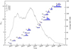 |
Fig. 2. Temporal evolution of all the CHs under study. The length of the bars represents the lifetime from the first to the last observation near the central meridian. The profile displays the area evolution (scale in the left corner of the figure). The red triangle marks the peak in the CH area. If no clear central peak was detected, the mark was omitted. The number in front of the bars shows how many times the CH was observed passing the central meridian. The solar activity, approximated by the smoothed sunspot number (Source: WDC-SILSO, Royal Observatory of Belgium, Brussels), is shown in the background. |
CHs with a lifetime from 5 to 18 rotations were observed. The two CHs with the longest lifetimes (17 and 18 rotations) were observed during the solar minimum (2017−2019) but this is obviously not a general trend. We note that this only regards CHs already considered long-living and in a sample where polar CHs are excluded. We almost continuously observe long-living CHs throughout the solar cycle with only one notable exception near the maximum in the solar activity (between 2014 and 2015).
3.2. Coronal hole evolution in A, Bs, and Φs
By examining a sample of 16 long-lived CHs throughout the SDO era, we found that 13 show a steady change in area, which is characterized by an approximately monotonic increase in the area followed by a roughly monotonic decrease (with scatter). Such a general trend is often visible, but the relative position of the peak, the maximum and minimum area, and the lifetime vary significantly. This demonstrates the individuality in the evolution of each CH. Figure 3 shows the evolution of the CH area (black-red) of all 16 studied CHs. The blue line represents the evolution of the photospheric magnetic flux density within the projected CH area. We note that large jumps in the area might be caused by merging or splitting with or into CHs, connection to polar CHs, or nearby filament eruptions that abruptly open additional field lines.
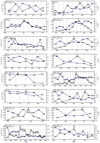 |
Fig. 3. Evolution of the area (black–red) and magnetic flux density (blue) of all CHs under study. The error bars represent the uncertainties. The vertical dashed guidelines represent the first day of each month and the yellow pin marks the peak in the observed CH area (if a clear peak was associated). |
CHs are usually considered to be large-scale structures that are defined by their magnetic field topology, the predominantly open field configuration. Therefore, we analyze the photospheric magnetic field underlying the extracted boundary to investigate the relation between magnetic field evolution and area evolution. As shown in Fig. 3, the evolution of the mean signed magnetic flux density of different CHs does not follow a uniform trend but displays various kinds of behavior. We find CHs that seem to have a visual correlation of area and flux density evolution as well as some with a supposed anti-correlation and ones without noticeable correlation. We quantify these correlations and anticorrelations below.
Figure 4 shows the average properties over each CHs evolution. We find only mild variations in the mean parameters (A*,Bs*,Φs*), represented by the mid-point of each vertical bar. However, the variations over each evolution may strongly vary. The CH areas over the entire CH evolution may vary slightly (∼2−3 × 10¹⁰ km2) or strongly (> 10 × 1010 km2) around the mean. We find magnetic flux densities ranging from ∼1 G up to ∼9 G with usual variations over the lifetime of a CH of about ±(1−2) G around the mean. The value of the mean magnetic flux of a CH over its evolution seems to be similar for all CHs, but the variation of the mean magnetic flux throughout individual the evolution seems to be on the order of the mean.
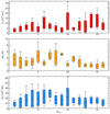 |
Fig. 4. Average properties over the evolution of each CH. The middle represents the average property (A*, Bs*, Φs*), the colored bar the 1σ range, and the whiskers show the full range of values of the parameter observed over the evolution. Top, middle, and bottom panels: CH area, CH flux density, and signed flux, respectively. |
3.3. Change rates
In addition to the evolutionary profile in the CH properties, we investigated the average rates at which CH properties change (a) in order to evaluate whether CHs evolve at similar rates or differ significantly from each other and (b) to gather important information on how the open magnetic field changes, as CHs are a major contributor of open magnetic flux (in regards to the open flux problem). Figure 5 shows the average change rates of the individual CH evolutions separated into growth rates (positive change rates, red) and decay rates (negative change rates, blue). Averaged over all CH evolutions, we find an area change rate (Fig. 5, top panel) of (14.2 ± 15.0)×108 km2 day−1 that can be divided into an area growth rate of (15.4 ± 18.5)×108 km2 day−1 and a similar area decay rate of (13.2 ± 12.6)×108 km2 day−1. This suggests that, on average, the CH grows and decays at a similar rate. We observe a possible solar cycle dependence of the area change rates, as in and near the solar maximum (2012−2014) we find change rates of (10.7 ± 8.9)×108 km2 day−1. During the descending phase and solar minimum (2016−2019) the average area change rates are higher at around (17.5 ± 18.7)×108 km2 day−1.
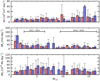 |
Fig. 5. Average change rates (growth: red; decay: blue) for each CH evolution individually. Top panel: average CH area change rates, middle: CH flux density change rates, and bottom panel: change rates of the signed flux. The purple triangles mark values calculated from only 1 or 2 measurement points, making them less reliable. |
The second panel in Fig. 5 shows the change rates for the mean signed magnetic flux density. We find similar rates for both growth and decay in each CHs evolution, on average 27.3 ± 32.2 mG day−1. We again observe a difference in the rates between CHs near solar maximum (2012−2014) and CHs near the solar minimum (2016−2019). During the former, the flux density increases at an average rate of 24.5 ± 25.1 mG day−1 and decreases at a similar rate of 30.9 ± 34.5 mG day−1. During the later interval, the change rates drop by up to a factor of two to 17.8 ± 18.8 mG day−1 for growth and 17.6 ± 16.8 mG day−1 for decay.
From the bottom panel of Fig. 5 we can deduce that the magnetic flux of a CH evolves at an average rate of (30.3 ± 31.5)×1018 Mx day−1. Interestingly, we find that for most CHs the average negative flux change rate is 20−30% higher than the average positive change rate. It is not clear whether this an effect dominated by the area evolution of a CH or by magnetic field evolution. All change rates of CH area, mean signed magnetic flux density, and magnetic flux are listed in Table 1.
Average change rates throughout the CH evolution. “max” denotes the time interval 2012−2014 and “min” the interval 2016−2019.
3.4. Correlations
After deriving various evolutionary CH parameters, we investigated possible correlations. Figure 6 shows the three primary CH properties (averaged over the CH lifetime), namely area (top, red), flux density (middle, orange) and flux (bottom, blue), and their change rates as a function of CH lifetime. We find moderate correlations between the average CH area (ccPearson = 0.52) and the average flux density (ccPearson = −0.46), albeit strongly influenced by the two very large and long-living CHs during solar minimum (two data points on the far right). No correlation with the CH lifetime is visible in the change rates or in the average magnetic flux.
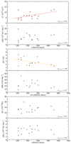 |
Fig. 6. Scatterplot of the average evolutionary CH properties and their absolute change rates against the CH lifetime. Top panel (red): CH area (A*, |dA|), middle panel (orange): mean signed magnetic flux density (Bs*, |dBs|), and bottom panel (blue): signed magnetic flux (Φs*, |dΦs|). |
Figure 7 investigates a possible dependence of average CH parameters and change rates on solar activity. The average sunspot number was used as a proxy for the solar activity. We define the average sunspot number in the evolution of a CH as the mean SIDC sunspot number over the time interval in which the CH was observed. We find weak (anti-)correlations between average CH area, flux density, and their change rates to solar activity. Parameters that show the highest correlation with solar activity are the average magnetic flux (ccPearson = 0.50) and the flux change rate (ccPearson = 0.69).
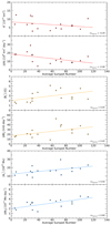 |
Fig. 7. Scatterplot of the average evolutionary CH properties and their absolute change rates against the average sunspot number as a proxy for solar activity. Top panel (red): CH area (A*, |dA|), middle panel (orange): mean signed magnetic flux density (Bs*, |dBs|), and bottom panel (blue): signed magnetic flux (Φs*, |dΦs|). |
Figure 8 shows CH area versus flux density. We find a weak anti-correlation for the whole sample (ccPearson = −0.33) and a strong anti-correlation for the averages (ccPearson = −0.70). We note that the strong anti-correlation between the average CH area and the mean magnetic flux density is attributable to a smoothing effect of the whole sample and is not a causal relation. Also, we find CHs in which the evolutionary profile of the area appears to be quite strongly correlated with the flux density evolution (3/16), some that show no correlation at all (6/16), and a significant proportion that show a weak to strong anti-correlation (7/16). We note here that the slopes of the regression line of some CH evolutions are very low due to an only slightly changing magnetic flux density throughout the lifetime. This can artificially enhance the Pearson correlation coefficient without a causal relation being present. All CHs retain the same polarity over their evolution. The change rates of CH area and flux density (Fig. 8, bottom panel) do not seem to be correlated (average over all evolutions: ccmean = −0.15).
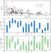 |
Fig. 8. Scatterplot of the absolute value of the signed mean magnetic flux density of CHs as a function of the CH area. Top panel: all observations (in red the average values over each evolution). Middle panel: evolution of each CH individually. Bottom panel: correlation between change in area and change in magnetic flux density for each CH evolution individually. Middle and bottom panels: the median of the bootstrapped sample for each evolution is represented by the horizontal line in the bar, the green and blue bars represent the 80% percentiles, and the whiskers the 90% percentiles. The dotted line gives the mean of the median values. |
3.5. High speed stream velocity evolution
Here we investigate whether or not the well-established CH area–HSS peak velocity relation is visible over individual CH evolutions. Using the geoeffective CH area calculated from Eq. (4), we derive a Pearson correlation coefficient of ccPearson = 0.46 with a 90% confidence interval of [0.36, 0.55] for the full sample. When considering each evolution individually, we find a large range of correlation coefficients between medium and strong correlations (see Fig. 9). Possible reasons for this are discussed below. The mean correlation coefficient of all 16 individual evolution correlation coefficients comes to ccmean = 0.59 ± 0.26. The slopes of the individual regression lines vary significantly around (3−44)×10−10 km−1 s−1 with accordingly different y-intercepts. For large CHs (A > 10 × 1010 km2) we find a saturation effect in the peak velocity. For “patchy” CHs (large fragmented CHs with weakly defined boundaries), the maximum peak velocity seems to be lower than one would expect for CHs with an area of this size. We investigated in-situ measured plasma density and magnetic field magnitude at the position of the velocity plateau and did not find any correlations to the CH area or magnetic field properties.
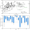 |
Fig. 9. Correlation plot of the CH area vs. the plateau bulk velocity of the associated HSS. Top panel: all observations and bottom panel: evolution of each individual CH. The green circle marks the “patchy” CHs that have large uncertainties in their area. Bottom panel: the median of the bootstrapped sample for each evolution is represented by the horizontal line in the bar, the green and blue bars represent the 80% percentiles, and the whiskers the 90% percentiles. The dotted line gives the mean values. |
4. Discussion
Using EUV full-disk observations by AIA and HMI magnetograms throughout most of the operational lifetime of SDO between 2010 and 2019 we studied the evolution of a sample of 16 long-living CHs and their associated HSSs.
We find that 13 out of 16 CHs follow a visible trend in the area evolution covering roughly one growing phase until a clear maximum is reached followed by a decay phase. Only 3 CHs show erratic behavior, for example revealing multiple peaks in the area or a maximum area at the birth or decay. From this we deduce that the majority of CHs (> 80%) undergo an area evolution that follows a pattern of growth and decay. However, we note that due to the small sample size we cannot comment on the significance of this finding. The proposed three-phase evolution (Heinemann et al. 2018a) might be rather the exception as it was only clearly observed for one CH.
We find a moderate correlation between the average CH area and flux density, but the correlation is not significant. Also, the change rates seem independent of the lifetime.
We find a correlation between solar activity and the average CH properties and their change rates. In particular, the change rate of the magnetic flux in CHs is strongly correlated with the average sunspot number during the CH life-time. We suspect that the open field of CHs is only able to expand in response to the magnetic activity (magnetic pressure) in quiet Sun areas and active regions in the vicinity.
Specifically, we found that near and during solar maximum (2012−2014), the area change rate was found to be (10.7 ± 8.9)×108 km2 day−1 (similar for both growth and decay rates) and during solar minimum the rate was around 60% larger at (17.5 ± 18.7)×108 km2 day−1. Our results for the solar maximum match the area change rates found by Bohlin (1977) of (13.0 ± 3.5)×108 km2 day−1 relatively well. Nolte et al. (1978a) used Skylab X-ray observations of long-living coronal holes during the descending phase of solar cycle 20 and derived rates of (7.3 ± 1.4)×108 km2 day−1, which is lower than the values found in the present study. Large deviations between the rates from previous studies can be primarily found in the CH evolutions during low solar activity where much larger average rates were derived. The growth and decay rates were found to be relatively stable across long-living CHs observed during times of similar solar activity. The consistent average rates suggest that discrete events that may cause sudden large-scale changes in the CHs, like filament eruptions that permanently open magnetic field lines (e.g., Kahler & Moses 1990), are rare events and that CHs evolve more gradually. This might explain the discrepancy between Nolte et al. (1978a), who claimed that most of the area evolution of a CH can be explained by discrete boundary changes of sizes larger than 2.7 × 10⁸ km2, and Kahler & Moses (1990) who found no such sudden large-scale changes. When comparing the average rate at which CHs evolve with results from flux transport calculations by Leighton (1964) we are in good agreement during the solar maximum but are not in agreement during low solar activity.
A similar picture can be deduced from the change rates of the mean signed magnetic flux density enclosed within the projected CH boundary. For evolutions of individual CHs, the rate at which the flux density changes stays at similar values but the percentage scatter is larger than in the area change rates. We show that the change rates of the flux density are higher during enhanced solar activity; for the time range of 2012−2014 (near and at solar maximum) we derive rates of (28 ± 30 mG day−1) and over 30% lower rates of 18 ± 17 mG day−1 near solar minimum (2016−2019). This hints towards a small imbalance between flux appearance and flux removal rates as well as low rates in general. Gošić et al. (2016) found average net flux density change rates of 5.0 ± 5.8 G day−1 in internetwork elements of two supergranular cells in the quiet Sun using 38 h of continuous HINODE observations. Smitha et al. (2017) report values about a factor of ten larger using SUNRISE data. We note that comparison should be treated cautiously as the rates derived by both Gošić et al. (2016) and Smitha et al. (2017) are from internetwork elements and the ones in this study are from the total extracted CH area. Also, HINODE and SUNRISE obtain their magnetograms at a much higher resolution and sensitivity than HMI/SDO which might explain the difference between the results gathered in this study and those found by the latter two mentioned authors.
Zhang et al. (2007) found that in a decaying CH a decrease of flux is caused by the emergence of opposite polarity flux within the CH boundaries and also that almost no flux transport is observed across the CH boundary. According to this, changes in the magnetic flux density in CHs are caused by processes within the CH boundaries, such as for example changes in flux emergence rate. The average CH area and average flux density over the CH evolutions seem to be correlated, however this is simply a smoothing effect and does not imply a causal correlation (see Fig. 8). From the statistical distribution of small unipolar magnetic elements within CHs that have been found to define the magnetic topology of a CH, it can be simply deduced that only smaller CHs might have higher flux densities (but also can have small flux density). Alternatively, in large CHs the flux density tends to converge to a mean flux density of about 1−3 G (see Heinemann et al. 2018b, 2019; Hofmeister et al. 2019). As such, the derived anti-correlation is not an evolutionary effect. Larger statistical studies of CH properties show no correlation between the CH area and its magnetic flux density (Hofmeister et al. 2017; Heinemann et al. 2019).
As such, the evolution of the magnetic flux density and magnetic flux cannot explain the evolutionary behavior of the CH area. We propose that the area evolution of CHs is not primarily caused by the evolution of the mean signed magnetic flux density within the projected CH boundary as extracted from EUV observations. Possible processes that might play a role in the area evolution include interchange reconnection (see Shelke & Pande 1984; Wang & Sheeley 2004; Madjarska et al. 2004; Fisk 2005; Madjarska & Wiegelmann 2009; Edmondson et al. 2010; Krista et al. 2011; Yang et al. 2011; Ma et al. 2014; Kong et al. 2018) and/or the change in the global and local magnetic field configuration outside the CH.
In addition to the evolutionary trend derived from remote sensing data, we investigated the evolution of the in-situ measured peak velocity of the associated HSS. Using the geoeffective CH area, we derive a mean correlation coefficient of the individual CH evolutions of ccPearson, mean = 0.59 ± 0.26, which is in the range of previous statistical studies of the CH area–HSS peak velocity relation (Karachik & Pevtsov 2011: ccPearson = 0.41 to 0.65; Vršnak et al. 2007; Abramenko et al. 2009; Verbanac et al. 2011a,b; Rotter et al. 2012; Tokumaru et al. 2017; Hofmeister et al. 2018: ccPearson = 0.62 to 0.80). Our results are also in good agreement with those of Heinemann et al. (2018a), who found a correlation coefficient of ccPearson = 0.77 in their case study of a long-living CH. We find a saturation effect in the peak velocity–CH area relation, where the peak velocity of large CHs does not follow a linear trend but rather converges to a speed of roughly 700 km s−1. This might be related to the longitudinal saturation found by Garton et al. (2018).
We conclude that the CH area–HSS peak velocity relation is clearly visible within the evolution of each CH, but the slopes of the linear regression lines vary significantly. We identify three possible causes for the varying slopes: (1) The in-situ measured bulk velocity depends not only on the CH but also on the preconditioning of the interplanetary space (e.g., Temmer et al. 2017). HSS or CMEs near or before the arrival of the HSS under study can significantly influence the measured speeds. This may lead to enhanced scatter in the relations. (2) The relation between CH area and HSS peak velocity is individual for each CH. (3) It might be possible that the CH area and the HSS peak velocity are not directly causally related. It is known that the geometry of CHs plays an important role in defining the 3D shape of the HSS (e.g., Garton et al. 2018).
5. Conclusions
In this statistical study, we investigate the evolution of 16 long-living CHs between 2010 and 2019 and the associated evolution of the HSS peak velocity at 1AU. Our major findings can be summarized as follows.
-
We find that the general CH area evolution (> 80% of the studied cases) exhibits a rough evolutionary profile showing a rise to a clear peak in the observed CH area followed by a decay.
-
The strength and evolution of the photospheric magnetic flux and flux density enclosed in the projected CH boundary is found to be largely independent of the evolution of the CH area. This suggests that the mean signed flux density of CHs is not the main cause for the observed evolution in the CH area.
-
Area growth and decay rates within CHs over their evolution seem to only vary over the solar cycle, with higher rates during lower solar activity. The calculated rates for the high solar activity match flux transport rates derived by Leighton (1964). Sudden large-scale changes in the area seem to be rare events.
-
The rates at which the magnetic flux and flux density change seem to be related to the activity of the Sun. We find higher rates during enhanced solar activity than during periods of low solar activity as approximated by the sunspot number.
-
We find no correlation between the CH area and the rate of change in magnetic flux density, suggesting that the rate at which the magnetic flux density of a CH evolves is independent of the area evolution of the CH and we suspect that this is caused by changes in the signed flux within the projected CH boundary (e.g., flux accumulation and cancellation due to flux emergence).
-
The well-known CH area–HSS relation is shown to persist over each individual CH evolution with varying correlation coefficients and varying slopes of the linear regression line.
Although an evolutionary trend was revealed in the general CH area evolution, the underlying magnetic mechanisms are still unclear. It can be deduced that an interplay of the magnetic configuration within and outside of the CH boundaries must play a major role. Future research on the 3D magnetic structure surrounding CHs might shed more light on this.
Royal Observatory of Belgium, Brussels: http://www.sidc.be/silso/
Acknowledgments
The SDO image data and the ACE in-situ data is available by courtesy of NASA and the respective science teams. S.G.H., M.T. and A.M.V. acknowledge funding by the Austrian Space Applications Programme of the Austrian Research Promotion Agency FFG (859729, SWAMI). V.J. acknowledges support from University of Zagreb, Croatia, Erasmus+ program. M.D. acknowledges support by the Croatian Science Foundation under the project 7549 (MSOC). S.J.H. thanks the OEAD for supporting this research by a Mariett-Blau-fellowship. S.G.H. would like to thank A.H.-P. for his endless supply of coffee, great motivation and helpful discussions.
References
- Abramenko, V., Yurchyshyn, V., & Watanabe, H. 2009, Sol. Phys., 260, 43 [NASA ADS] [CrossRef] [Google Scholar]
- Acuña, M. H., Ogilvie, K. W., Baker, D. N., et al. 1995, Space Sci. Rev., 71, 5 [NASA ADS] [CrossRef] [Google Scholar]
- Alves, M. V., Echer, E., & Gonzalez, W. D. 2006, J. Geophys. Res. (Space Phys.), 111, A07S05 [CrossRef] [Google Scholar]
- Bale, S., Badman, S., Bonnell, J., et al. 2019, Nature, 576, 237 [NASA ADS] [CrossRef] [Google Scholar]
- Bohlin, J. D. 1977, Sol. Phys., 51, 377 [NASA ADS] [CrossRef] [Google Scholar]
- Bohlin, J. D., & Sheeley, N. R., Jr. 1978, Sol. Phys., 56, 125 [CrossRef] [Google Scholar]
- Couvidat, S., Schou, J., Hoeksema, J. T., et al. 2016, Sol. Phys., 291, 1887 [Google Scholar]
- Cranmer, S. R. 2009, Liv. Rev. Sol. Phys., 6, 3 [Google Scholar]
- Domingo, V., Fleck, B., & Poland, A. I. 1995, Sol. Phys., 162, 1 [NASA ADS] [CrossRef] [Google Scholar]
- Edmondson, J. K., Antiochos, S. K., DeVore, C. R., Lynch, B. J., & Zurbuchen, T. H. 2010, ApJ, 714, 517 [NASA ADS] [CrossRef] [Google Scholar]
- Efron, B. 1979, Ann. Stat., 7, 1 [Google Scholar]
- Efron, B., & Tibshirani, R. J. 1993, An Introduction to the Bootstrap (New York: Chapman & Hall) [Google Scholar]
- Fisk, L. A. 2005, ApJ, 626, 563 [Google Scholar]
- Garton, T. M., Gallagher, P. T., & Murray, S. A. 2018, J. Space Weather Space Clim., 8, A02 [CrossRef] [EDP Sciences] [Google Scholar]
- Gibson, S. E., Biesecker, D., Guhathakurta, M., et al. 1999, ApJ, 520, 871 [NASA ADS] [CrossRef] [Google Scholar]
- Gopalswamy, N., Shibasaki, K., Thompson, B. J., Gurman, J., & DeForest, C. 1999, J. Geophys. Res., 104, 9767 [NASA ADS] [CrossRef] [Google Scholar]
- Gosling, J. T. 1996, ARA&A, 34, 35 [NASA ADS] [CrossRef] [Google Scholar]
- Gošić, M., Bellot Rubio, L. R., del Toro Iniesta, J. C., Orozco Suárez, D., & Katsukawa, Y. 2016, ApJ, 820, 35 [NASA ADS] [CrossRef] [Google Scholar]
- Harvey, K. L., Sheeley, N. R., Jr., & Harvey, J. W. 1982, Sol. Phys., 79, 149 [NASA ADS] [CrossRef] [Google Scholar]
- Heinemann, S. G., Temmer, M., Hofmeister, S. J., Veronig, A. M., & Vennerstrøm, S. 2018a, ApJ, 861, 151 [NASA ADS] [CrossRef] [Google Scholar]
- Heinemann, S. G., Hofmeister, S. J., Veronig, A. M., & Temmer, M. 2018b, ApJ, 863, 29 [NASA ADS] [CrossRef] [Google Scholar]
- Heinemann, S. G., Temmer, M., Heinemann, N., et al. 2019, Sol. Phys., 294, 144 [CrossRef] [Google Scholar]
- Hofmeister, S. J., Veronig, A., Reiss, M. A., et al. 2017, ApJ, 835, 268 [NASA ADS] [CrossRef] [Google Scholar]
- Hofmeister, S. J., Veronig, A., Temmer, M., et al. 2018, J. Geophys. Res. (Space Phys.), 123, 1738 [NASA ADS] [Google Scholar]
- Hofmeister, S. J., Utz, D., Heinemann, S. G., Veronig, A. M., & Temmer, M. 2019, A&A, 629, A22 [CrossRef] [EDP Sciences] [Google Scholar]
- Ikhsanov, R. N., & Tavastsherna, K. S. 2015, Geomagn. Aerono., 55, 877 [NASA ADS] [CrossRef] [Google Scholar]
- Jian, L., Russell, C. T., Luhmann, J. G., & Skoug, R. M. 2006, Sol. Phys., 239, 337 [NASA ADS] [CrossRef] [Google Scholar]
- Jian, L. K., Russell, C. T., Luhmann, J. G., Galvin, A. B., & MacNeice, P. J. 2009, Sol. Phys., 259, 345 [NASA ADS] [CrossRef] [Google Scholar]
- Kahler, S. W., & Moses, D. 1990, ApJ, 362, 728 [NASA ADS] [CrossRef] [Google Scholar]
- Karachik, N. V., & Pevtsov, A. A. 2011, ApJ, 735, 47 [CrossRef] [Google Scholar]
- Kong, D. F., Pan, G. M., Yan, X. L., Wang, J. C., & Li, Q. L. 2018, ApJ, 863, L22 [CrossRef] [Google Scholar]
- Krieger, A. S., Timothy, A. F., & Roelof, E. C. 1973, Sol. Phys., 29, 505 [NASA ADS] [CrossRef] [Google Scholar]
- Krista, L. D., Gallagher, P. T., & Bloomfield, D. S. 2011, ApJ, 731, L26 [NASA ADS] [CrossRef] [Google Scholar]
- Leighton, R. B. 1964, ApJ, 140, 1547 [Google Scholar]
- Lemen, J. R., Title, A. M., Akin, D. J., et al. 2012, Sol. Phys., 275, 17 [NASA ADS] [CrossRef] [Google Scholar]
- Lowder, C., Qiu, J., & Leamon, R. 2017, Sol. Phys., 292, 18 [NASA ADS] [CrossRef] [Google Scholar]
- Ma, L., Qu, Z.-Q., Yan, X.-L., & Xue, Z.-K. 2014, Res. Astron. Astrophys., 14, 221 [CrossRef] [Google Scholar]
- Madjarska, M. S., & Wiegelmann, T. 2009, A&A, 503, 991 [NASA ADS] [CrossRef] [EDP Sciences] [Google Scholar]
- Madjarska, M. S., Doyle, J. G., & van Driel-Gesztelyi, L. 2004, ApJ, 603, L57 [NASA ADS] [CrossRef] [Google Scholar]
- Neugebauer, M., Liewer, P. C., Smith, E. J., Skoug, R. M., & Zurbuchen, T. H. 2002, J. Geophys. Res. (Space Phys.), 107, 1488 [Google Scholar]
- Nolte, J. T., Krieger, A. S., Timothy, A. F., et al. 1976, Sol. Phys., 46, 303 [NASA ADS] [CrossRef] [Google Scholar]
- Nolte, J. T., Gerassimenko, M., Krieger, A. S., & Solodyna, C. V. 1978a, Sol. Phys., 56, 153 [NASA ADS] [CrossRef] [Google Scholar]
- Nolte, J. T., Krieger, A. S., & Solodyna, C. V. 1978b, Sol. Phys., 57, 129 [NASA ADS] [CrossRef] [Google Scholar]
- Pesnell, W. D., Thompson, B. J., & Chamberlin, P. C. 2012, Sol. Phys., 275, 3 [NASA ADS] [CrossRef] [Google Scholar]
- Petrie, G. J. D., & Haislmaier, K. J. 2013, ApJ, 775, 100 [NASA ADS] [CrossRef] [Google Scholar]
- Richardson, I. G. 2018, Liv. Rev. Sol. Phys., 15, 1 [Google Scholar]
- Richardson, I. G., & Cane, H. V. 2010, Sol. Phys., 264, 189 [NASA ADS] [CrossRef] [Google Scholar]
- Rotter, T., Veronig, A. M., Temmer, M., & Vršnak, B. 2012, Sol. Phys., 281, 793 [NASA ADS] [CrossRef] [Google Scholar]
- Schou, J., Scherrer, P. H., Bush, R. I., et al. 2012, Sol. Phys., 275, 229 [Google Scholar]
- Shelke, R. N., & Pande, M. C. 1984, Bull. Astron. Soc. India, 12, 404 [NASA ADS] [Google Scholar]
- Smitha, H. N., Anusha, L. S., Solanki, S. K., & Riethmüller, T. L. 2017, ApJS, 229, 17 [NASA ADS] [CrossRef] [EDP Sciences] [Google Scholar]
- Stone, E. C., Frandsen, A. M., Mewaldt, R. A., et al. 1998, Space Sci. Rev., 86, 1 [Google Scholar]
- Temmer, M., Reiss, M. A., Nikolic, L., Hofmeister, S. J., & Veronig, A. M. 2017, ApJ, 835, 141 [Google Scholar]
- Tokumaru, M., Satonaka, D., Fujiki, K., Hayashi, K., & Hakamada, K. 2017, Sol. Phys., 292, 41 [Google Scholar]
- Tsurutani, B. T., Gonzalez, W. D., Gonzalez, A. L. C., et al. 2006, J. Geophys. Res. (Space Phys.), 111, A07S01 [NASA ADS] [Google Scholar]
- Verbanac, G., Vršnak, B., Živković, S., et al. 2011a, A&A, 533, A49 [NASA ADS] [CrossRef] [EDP Sciences] [Google Scholar]
- Verbanac, G., Vršnak, B., Veronig, A., & Temmer, M. 2011b, A&A, 526, A20 [Google Scholar]
- Verbeeck, C., Delouille, V., Mampaey, B., & De Visscher, R. 2014, A&A, 561, A29 [NASA ADS] [CrossRef] [EDP Sciences] [Google Scholar]
- Vršnak, B., Temmer, M., & Veronig, A. M. 2007, Sol. Phys., 240, 315 [Google Scholar]
- Vršnak, B., Dumbović, M., Čalogović, J., Verbanac, G., & Poljančić Beljan, I. 2017, Sol. Phys., 292, 140 [Google Scholar]
- Wang, Y.-M., & Sheeley, N. R., Jr. 1990, ApJ, 355, 726 [Google Scholar]
- Wang, Y. M., & Sheeley, N. R., Jr. 2004, ApJ, 612, 1196 [NASA ADS] [CrossRef] [Google Scholar]
- Webb, D. F., Nolte, J. T., Solodyna, C. V., & McIntosh, P. S. 1978, Sol. Phys., 58, 389 [NASA ADS] [CrossRef] [Google Scholar]
- Wilcox, J. M. 1968, Space Sci. Rev., 8, 258 [Google Scholar]
- Yang, S., Zhang, J., & Borrero, J. M. 2009, ApJ, 703, 1012 [NASA ADS] [CrossRef] [Google Scholar]
- Yang, S., Zhang, J., Li, T., & Liu, Y. 2011, ApJ, 732, L7 [NASA ADS] [CrossRef] [Google Scholar]
- Yermolaev, Y. I., Lodkina, I. G., Nikolaeva, N. S., et al. 2018, J. Atmos. Sol.-Terr. Phys., 180, 52 [NASA ADS] [CrossRef] [Google Scholar]
- Zhang, J., Zhou, G., Wang, J., & Wang, H. 2007, ApJ, 655, L113 [NASA ADS] [CrossRef] [Google Scholar]
Appendix A: Snapshot of coronal holes under study
Figure A.1 shows a snapshot of every coronal hole analyzed in this study. The red line represents the extracted CH boundary using CATCH and the yellow x is the center of mass.
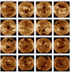 |
Fig. A.1. Example snapshot of CH under study. The extracted CH boundary is given by the red line and the center of mass is represented by the yellow x. The blue shaded areas represent the uncertainties as calculated by CATCH. |
All Tables
Average change rates throughout the CH evolution. “max” denotes the time interval 2012−2014 and “min” the interval 2016−2019.
All Figures
|
Fig. 1. Example of an in-situ signature of the solar wind data provided by the OMNI database (left), as a CH under study was observed near the center of the solar disk by SDO on May 29, 2013, at 18 UT (right). The black line shows the solar wind bulk velocity and green line represents the plasma density. The purple triangle represents the peak velocity and the horizontal bar the average interval to show the plateau speed. The colored bar on the top represents the in-situ polarity calculated after Neugebauer et al. (2002), with red being positive and blue negative polarity. Right panel: snapshot of the CH that is associated with this HSS, and the time of the SDO observation corresponds to the yellow vertical line in the left panel. The red line is the extracted CH boundary (using CATCH) and the yellow x represents the center of mass of the CH. |
| In the text | |
|
Fig. 2. Temporal evolution of all the CHs under study. The length of the bars represents the lifetime from the first to the last observation near the central meridian. The profile displays the area evolution (scale in the left corner of the figure). The red triangle marks the peak in the CH area. If no clear central peak was detected, the mark was omitted. The number in front of the bars shows how many times the CH was observed passing the central meridian. The solar activity, approximated by the smoothed sunspot number (Source: WDC-SILSO, Royal Observatory of Belgium, Brussels), is shown in the background. |
| In the text | |
|
Fig. 3. Evolution of the area (black–red) and magnetic flux density (blue) of all CHs under study. The error bars represent the uncertainties. The vertical dashed guidelines represent the first day of each month and the yellow pin marks the peak in the observed CH area (if a clear peak was associated). |
| In the text | |
|
Fig. 4. Average properties over the evolution of each CH. The middle represents the average property (A*, Bs*, Φs*), the colored bar the 1σ range, and the whiskers show the full range of values of the parameter observed over the evolution. Top, middle, and bottom panels: CH area, CH flux density, and signed flux, respectively. |
| In the text | |
|
Fig. 5. Average change rates (growth: red; decay: blue) for each CH evolution individually. Top panel: average CH area change rates, middle: CH flux density change rates, and bottom panel: change rates of the signed flux. The purple triangles mark values calculated from only 1 or 2 measurement points, making them less reliable. |
| In the text | |
|
Fig. 6. Scatterplot of the average evolutionary CH properties and their absolute change rates against the CH lifetime. Top panel (red): CH area (A*, |dA|), middle panel (orange): mean signed magnetic flux density (Bs*, |dBs|), and bottom panel (blue): signed magnetic flux (Φs*, |dΦs|). |
| In the text | |
|
Fig. 7. Scatterplot of the average evolutionary CH properties and their absolute change rates against the average sunspot number as a proxy for solar activity. Top panel (red): CH area (A*, |dA|), middle panel (orange): mean signed magnetic flux density (Bs*, |dBs|), and bottom panel (blue): signed magnetic flux (Φs*, |dΦs|). |
| In the text | |
|
Fig. 8. Scatterplot of the absolute value of the signed mean magnetic flux density of CHs as a function of the CH area. Top panel: all observations (in red the average values over each evolution). Middle panel: evolution of each CH individually. Bottom panel: correlation between change in area and change in magnetic flux density for each CH evolution individually. Middle and bottom panels: the median of the bootstrapped sample for each evolution is represented by the horizontal line in the bar, the green and blue bars represent the 80% percentiles, and the whiskers the 90% percentiles. The dotted line gives the mean of the median values. |
| In the text | |
|
Fig. 9. Correlation plot of the CH area vs. the plateau bulk velocity of the associated HSS. Top panel: all observations and bottom panel: evolution of each individual CH. The green circle marks the “patchy” CHs that have large uncertainties in their area. Bottom panel: the median of the bootstrapped sample for each evolution is represented by the horizontal line in the bar, the green and blue bars represent the 80% percentiles, and the whiskers the 90% percentiles. The dotted line gives the mean values. |
| In the text | |
|
Fig. A.1. Example snapshot of CH under study. The extracted CH boundary is given by the red line and the center of mass is represented by the yellow x. The blue shaded areas represent the uncertainties as calculated by CATCH. |
| In the text | |
Current usage metrics show cumulative count of Article Views (full-text article views including HTML views, PDF and ePub downloads, according to the available data) and Abstracts Views on Vision4Press platform.
Data correspond to usage on the plateform after 2015. The current usage metrics is available 48-96 hours after online publication and is updated daily on week days.
Initial download of the metrics may take a while.