| Issue |
A&A
Volume 638, June 2020
|
|
|---|---|---|
| Article Number | A105 | |
| Number of page(s) | 26 | |
| Section | Interstellar and circumstellar matter | |
| DOI | https://doi.org/10.1051/0004-6361/201936118 | |
| Published online | 23 June 2020 | |
Probing the initial conditions of high-mass star formation
IV. Gas dynamics and NH2D chemistry in high-mass precluster and protocluster clumps★
1
National Astronomical Observatories, Chinese Academy of Sciences,
100101
Beijing,
PR China
e-mail: cpzhang@nao.cas.cn
2
CAS Key Laboratory of FAST, National Astronomical Observatories, Chinese Academy of Sciences,
100101
Beijing,
PR China
3
Max-Planck-Institut für Astronomie,
Königstuhl 17,
69117
Heidelberg,
Germany
4
South-Western Institute for Astronomy Research, Yunnan University,
Kunming,
650500
Yunnan,
PR China
5
Institute for Astrophysical Research, 725 Commonwealth Ave, Boston University,
Boston,
MA
02215,
USA
6
Max-Planck-Institut für Radioastronomie,
Auf dem Hügel 69,
53121
Bonn,
Germany
7
Istituto di Fisica dello Spazio Interplanetario – INAF,
Via Fosso del Cavaliere 100,
00133
Roma,
Italy
Received:
17
June
2019
Accepted:
29
April
2020
Context. The initial stage of star formation is a complex area of study because of the high densities (nH2 > 106 cm−3) and low temperatures (Tdust < 18 K) involved. Under such conditions, many molecules become depleted from the gas phase by freezing out onto dust grains. However, the deuterated species could remain gaseous under these extreme conditions, which would indicate that they may serve as ideal tracers.
Aims. We investigate the gas dynamics and NH2D chemistry in eight massive precluster and protocluster clumps (G18.17, G18.21, G23.97N, G23.98, G23.44, G23.97S, G25.38, and G25.71).
Methods. We present NH2D 111–101 (at 85.926 GHz), NH3 (1, 1), and (2, 2) observations in the eight clumps using the PdBI and the VLA, respectively. We used 3D GAUSSCLUMPS to extract NH2D cores and provide a statistical view of their deuterium chemistry. We used NH3 (1, 1) and (2, 2) data to investigate the temperature and dynamics of dense and cold objects.
Results. We find that the distribution between deuterium fractionation and kinetic temperature shows a number density peak at around Tkin = 16.1 K and the NH2D cores are mainly located at a temperature range of 13.0 to 22.0 K. The 3.5 mm continuum cores have a kinetic temperature with a median width of 22.1 ± 4.3 K, which is obviously higher than the temperature in NH2D cores. We detected seven instances of extremely high deuterium fractionation of 1.0 ≤ Dfrac ≤ 1.41. We find that the NH2D emission does not appear to coincide exactly with either dust continuum or NH3 peak positions, but it often surrounds the star-formation active regions. This suggests that the NH2D has been destroyed by the central young stellar object (YSO) due to heating. The detected NH2D lines are very narrow with a median width of 0.98 ± 0.02 km s−1, which is dominated by non-thermal broadening. The extracted NH2D cores are gravitationally bound (αvir < 1), they are likely to be prestellar or starless, and can potentially form intermediate-mass or high-mass stars in future. Using NH3 (1, 1) as a dynamical tracer, we find evidence of very complicated dynamical movement in all the eight clumps, which can be explained by a combined process with outflow, rotation, convergent flow, collision, large velocity gradient, and rotating toroids.
Conclusions. High deuterium fractionation strongly depends on the temperature condition. Tracing NH2D is a poor evolutionary indicator of high-mass star formation in evolved stages, but it is a useful tracer in starless and prestellar cores.
Key words: stars: formation / techniques: interferometric / ISM: clouds / methods: observational
The reduced datacubes are only available at the CDS via anonymous ftp to cdsarc.u-strasbg.fr (130.79.128.5) or via http://cdsarc.u-strasbg.fr/viz-bin/cat/J/A+A/638/A105
© ESO 2020
1 Introduction
High-mass (≥ 8 M⊙) stars dominate the Galactic environment and its evolution but many aspects of their formation are still unclear (Shu et al. 1987; Churchwell 2002; Fuller et al. 2005; Bergin & Tafalla 2007; Zinnecker & Yorke 2007; Zhang et al. 2018). Firstly, the short time scales of high-mass protostellar objects and their large distances make it difficult to characterize their evolutionary stages. Secondly, star formation in the early stage takes place at the densest and coldest clumps (Pillai et al. 2007, 2011). At high densities ( 106 cm−3) and low temperatures (Tdust < 18 K), characteristic of the interiors of star-forming cores, many molecules are depleted from the gas phase by freezing out onto dust grain surfaces (Walmsley et al. 2004; Bergin & Tafalla 2007). Fortunately, the deuterium fractionation of the remaining gas-phase species increases dramatically above the cosmic [D/H] abundance ratio of ~1.5 × 10⁻⁵ (Oliveira et al. 2003) due to increased production of H2 D+ through the reaction of H
 with HD in places where CO is depleted (Roberts & Millar 2000). Deuterated molecules, particularly of N-bearing species, can thus serve as selective tracers of the coldest, densest gas in molecular clouds and star-forming cores (Friesen et al. 2018). Therefore, using deuterated species as tracers to probe the initial conditions of high-mass star formation is very useful.
Ammonia and its deuterated isotopologues are formed on grain surfaces through H/D-atom addition reactions to N atoms (Brown & Millar 1989a,b; Fedoseev et al. 2015a) and in the gas phase by reactions with deuterated ions convert part of NH3 to NH2 D, NHD2, and ND3 (Rodgers & Charnley 2001; Pillai et al. 2007). Substantial deuteration in both phases occurs after the disappearance of CO from the gas phase. It is likely that the relative abundances of the mentioned molecules could give us an idea of the evolutionary stage of a dense core, for example [N2 D+]/[N2H+], [NH2 D]/[NH3], and [ND3 ]/[NHD2] (Crapsi et al. 2005; Roueff et al. 2005; Flower et al. 2006; Pillai et al. 2007; Pagani et al. 2009; Daniel et al. 2016a). Harju et al. (2017) presented principal reactions forming and destroying NH2 D at the deuteration peak. The abundance of NH2D starts to increase gradually, first through the deuteron transfer to ammonia, primarily by HCND+ or DCNH+. The depletion of CO boosts the abundance of H , which, in turn, is efficiently deuterated to H2 D+, D2 H+, and D
 in successive reactions with HD. This stage is characterized by a rapid increase of N-bearing deuterated isotopologues. A detailed deuteration reaction network has been presented in more detail in Sipilä et al. (2015a,b).
Global organized bulk motions are ubiquitously observed in many star-forming regions with different evolutionary stages, for example, stellar wind in an infrared dust bubble (Zhang et al. 2013, 2016, 2019b) and supernova remnant (Zhou et al. 2016a,b), outflow driven by a powerful jet, large scale flow along a filament (Peretto et al. 2014; Lu et al. 2018; Yuan et al. 2018), and cloud–cloud collisions (Gong et al. 2017; Fukui et al. 2018). This suggests that the large-scale (≳ 1 pc) dynamics associated with massive star formation could shape the molecular structure. Additionally, the small-scales (≲ 1 pc) motion could be identified by rotation, inflow, and flow in fiber (Keto 2007; Galván-Madrid et al. 2009; Csengeri et al. 2011a,b; Zhang et al. 2014). The complicated dynamical processes in different scales are linked to the formation of morphological structure and final mass of central star. Therefore, the gas dynamics associated with star formation warrants further study.
In this work, we mainly report gas dynamics using NH3 (1, 1) and (2, 2), and we study o-NH2D 111 –101 chemistry in eight high-mass star-forming regions (G18.17, G18.21, G23.97N, G23.98, G23.44, G23.97S, G25.38, and G25.71). Four sources are infrared quiet and in a relatively early evolutionary stage, and the other four sources belong to evolved objects with embedded H II regions. The sample selection and source properties are listed in Table 1 (see also details in Zhang et al. 2019a). In followed Sect. 2, we describe the Plateau de Bure Interferometer (PdBI) and the Very Large Array (VLA) observations and data reduction. In Sect. 3, we show observational results of NH3 and NH2 D lines. In Sect. 4, source extraction, optical depth, kinetic temperature, density, velocity dispersion, mass, and virial stability are presented and analyzed. In Sect. 5, we discuss gas dynamics and deuterium chemistry. In Sect. 6, we give a summary.
Properties of selected sample.
2 Observations and data reduction
The IRAM1 PdBI and NRAO2 VLA observations at 1.3, 3.5, and 1.3 cm continuum have been described and presented in Zhang et al. (2019a). Here we expand on the spectral observations and data.
2.1 PdBI observations
The spectra in the PdBI observations were observed simultaneously along with the continuum in Mar. 25–Apr. 12, 2005 and Feb. 27–Mar. 17, 2006 (see details in Zhang et al. 2019a), but in separated correlator windows. Receiver 1 for covering the 111 –101 lines of o-NH2D at 85.926 GHz was tuned to 40 MHz bandwidth with 460 channels, leading to a velocity resolution of around 0.27 km s−1 per channel. The rms noise of spectra was around 23 mJy beam−1 for NH2D in the C+D configuration observations in sources G18.17, G18.21, G23.97N, G23.98, and G25.71, and around 12 mJy beam−1 for NH2D in the B+C+D configuration observations in sources G23.44, G23.97S, and G25.38 (see also Table 2).
The IRAM software package GILDAS3 was used for the data reduction. The continuum contributions were subtracted from the spectral uv-table data sets, which were then cleaned with natural weighting, and imaged to obtain spectral images and maps. The region of a twice primary beam size was searched for cleaning components. No polygon was introduced to avoid any biased cleaning. The primary beam was around 58.5″ at 86.086 GHz. The data have been corrected for primary beam attenuation. The detailed observations, data calibration and reduction have been presented in Zhang et al. (2019a).
Parameters of the PdBI and VLA observations: phase center, beam, and rms.
2.2 VLA observations
The spectra (J, K) = (1, 1) and (2, 2) transitions of NH3 were simultaneously covered in the eight clumps, using the 2-IF spectral line mode of the correlator with NRAO2 VLA D-configuration on November 2005 (project ID AW0669). The bandwidth was 6.25 MHz, with 127 channels of around 49 kHz (~0.617 km s−1) each. The NH3 (1, 1) and (2, 2) transitions have five and three hyperfine structure (HfS) lines, respectively, and the frequencies of the strongest HfS lines are at 23.6945 and 23.7263 GHz, respectively. Due to a narrow bandwidth of 6.25 MHz at around 23.7 GHz, it can just cover, at most, four HfS lines in five NH3 (1, 1). The primary beam was about 2′, and the typical synthesized beam size was about 3.0″ × 2.5″ at 1.3 cm. The raw data from the observations was exported to MIRIAD4 and GILDAS by AIPS5 for calibration and imaging. The spectra and continuum were calibrated with primary beam correction. The rms noise of the spectra was between 2.5 and 3.5 mJy beam−1 for NH3 (1, 1) and (2, 2) data (see also Table 2). The detailed observations, data calibration, and reduction can be found in Zhang et al. (2019a).
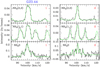 |
Fig. 1 Spectra NH2D, NH3 (1, 1) and (2,2) overlaid with their HfS fits for the first two NH2D cores (see Table A.2). The spectra are derived by averaging the lines within each NH2D core scale. Other sources and spectra are presented in Fig A.1. |
Parameters of o-NH2D HfS lines.
3 Observational results
3.1 NH2D
The 111 –101 transitions of o-NH2D at around 85.926 GHz have six HfS lines (Tiné et al. 2000; Müller et al. 2005; Daniel et al. 2016b). However, two of them blend into one at current spectral resolution (see Fig. 1). Therefore, we can only distinguish its five emission lines. Table 3 lists their frequencies, relative velocities, and relative intensities in theoretical calculations (Tiné et al. 2000).
The NH2D cores are extracted with 3D GAUSSCLUMPS algorithm (see Sect. 4.1). The core positions and sizes are indicated using green ellipses with core numbers in Fig. 2. The NH2D spectra of only the first two cores are shown in Fig. 1 for source G23.44 (other sources are shown in Fig. A.1), but the whole corresponding parameters are listed in Table A.2 including velocity, line width, brightness temperature, and opacity6. We also present the integrated-intensity contours of NH2D superimposed on the 3.5 mm continuum emission image in Fig. 2, and on the NH3 (1, 1) integrated-intensity maps in Fig. 3. The integrated velocity range covers all the six HfS lines of the NH2D (Tiné et al. 2000). We find thatthe NH2D peak positions are often not consistent with the 3.5 mm emission, and there exist obvious offsets between them. In Figs. 4 and 5, the integrated-intensity contours of the NH2D are also overlaid on line-center velocity and line-width maps of the NH3 (1, 1) for further investigating their dynamics.
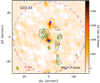 |
Fig. 2 NH2D integrated-intensity contours overlaid on a 3.5 mm continuum with velocity range covering all the six HfS lines. The contour levels start at − 3σ in steps of 3σ for NH2D with σ = 33.6 mJy beam−1km s−1. The green ellipses with red numbers indicate the positions of extracted NH2D cores. The symbols “▴”, “■”, and “⋆” indicate the positions of masers, H II regions, and infrared sources, respectively. The synthesized beam sizes are indicated at the bottom-left corner. The dashed circle indicates the primary beam of the PdBI observations at 3.5 mm. Other sources are presented in Fig. A.2. |
3.2 NH3 (1, 1) and (2, 2)
In Fig. 1, we also present the spectra of NH3 (1, 1) and (2, 2) from each corresponding NH2D core (see Sect. 4.1). These spectra were derived from the average within a corresponding core size. In Table A.2, we list their line width and brightness temperature by spectral Gaussian fitting derived in assumption of local thermodynamic equilibrium (LTE) conditions. In our previous work, Zhang et al. (2019a), we present the integrated-intensity contours of NH3 (1, 1) and (2, 2) overlaying on a 3.5 mm emission image, respectively. The NH3 peak positions are almost consistent with the 3.5 mm emission, but the NH3 (1, 1) and (2, 2) have much more extended structure than the 3.5 mm emission distribution. This is mainly because, independent of observations7, the 3.5 mm continuum might be more compact because of the internal heating sources, and NH3 is also optically thick, as we show in Table 2, which also means it is possible to see more extended NH3 emission.
In Fig. 4, we present velocity distributions (moment 1) of NH3 (1, 1) superimposed on NH2D emission. It is very obvious that there is a steep velocity gradient in the eight molecular clumps, such as G18.17 and 23.97N in east-west direction, G23.44, G25.38, and G25.71 in north-south direction, and the other sources (G23.98 and G23.97S) having two velocity components crossing into together. In Fig. 5, we present line width distribution (moment 2) of NH3 (1, 1) line overlaid with integrated-intensity contours (moment 0) of NH2D line. We can see that three high-mass star forming regions (G23.44, G23.97S, and G25.38) have clearly NH2D emission offset from the largest line broadening, indicating that the NH2D emission is often devoid of the dynamically dominated and active regions. Figures 6 and A.6 show the spectra NH3 (1, 1) and (2, 2) at the peak position of 3.5 mm continuum distribution for each source. The NH3 (1, 1) and (2, 2) lines present high velocity (wings) emission. The integrated-intensity maps of the blue- and red-shifted spectral wings of NH3 (1, 1) are shown in Figs. 7 and A.7, where the background is 3.5 mm emission. To judge the possibility of outflow or rotation movements, Figs. 8 and A.8 show their position-velocity diagrams using the main HfS line of NH3 (1, 1) along the position-velocity slice indicated with the solid and dashed lines in Figs. 7 and A.7, respectively.
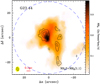 |
Fig. 3 NH2D integrated-intensity contours overlaid on an NH3 (1, 1) integrated-intensity image with velocity range covering all the six HfS lines. The contour levels start at − 3σ in steps of 3σ for NH2D with σ = 33.6 mJy beam−1km s−1. The synthesized beam sizes are indicated at the bottom-left corner. The dashed circle indicates the primary beam of the PdBI observations at 3.5 mm. Other sources are presented in Fig. A.3. |
4 Analysis
4.1 NH2D core extraction
Assuming that the flux density of each NH2D core can be approximated by a Gaussian distribution, the three dimensional (3D) GAUSSCLUMPS procedure (Stutzki & Guesten 1990; Kramer et al. 1996, 1998) in the GILDAS software package was used to characterize them. This methodology has been described in detail and successfully applied in Kramer et al. (1996, 1998). We consider the sources with line intensity above 5σ (see σ in Table 2) before primary beam correction and line width more than three channels, and fit a Gaussian shaped 3D core with Gaussian size larger than beam size to the surrounding region. For sources G18.17, G18.21, G23.97N, G23.98, and G25.71, we identify NH2D cores using CD configuration observations, and for sources G23.44, G23.97S, and G25.38, we identify them using BCD configuration observations. The identified cores are overlaid onto 2D integrated intensity maps (see Figs. 2 and A.2). The velocity, line width, brightness temperature, and opacity are derived from the spectral average within the measured Gaussian size of each core by fitting the HfS lines of NH2D and NH3. The detailed extraction steps are also presented in Zhang et al. (2019a). The core parameters are listed in Tables A.2 and A.3.
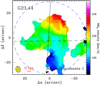 |
Fig. 4 Velocity distribution (moment 1) of NH3 (1, 1) line overlaid with integrated-intensity contours (moment 0) of NH2D line with velocity range covering all the six HfS lines. The contour levels start at − 3σ in steps of 3σ for NH2D with σ = 84.1 mJy beam−1km s−1. The synthesized beam sizes are indicated at the bottom-left corner. The dashed circle indicates the primary beam of the PdBI observations at 3.5 mm. The lines with arrows show the position-velocity cutting direction in Fig. 8. Other sources are presented in Fig. A.4. |
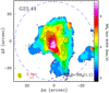 |
Fig. 5 Line width distribution (moment 2) of NH3 (1, 1) line overlaid with integrated-intensity contours (moment 0) of NH2D line with velocity range covering all the six HfS lines. The contour levels start at − 3σ in steps of 3σ for NH2D with σ = 84.1 mJy beam−1km s−1. The synthesized beam sizes are indicated at the bottom-left corner. The dashed circle indicates the primary beam of the PdBI observations at 3.5 mm. Other sources are presented in Fig. A.5. |
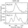 |
Fig. 6 Spectra NH3 (1, 1) and (2, 2) obtained toward a single and the brightest pixel at 3.5 mm continuum. The coordinates of the spectra are indicated at the lower panel of Fig. 8. Other sources are presented in Fig. A.6. |
4.2 HfS fitting
The transitions of NH3 (1, 1) and (2, 2) at around 23.6945 and 23.7263 GHz have five and three groups of HfS lines (Kukolich 1967; Ho 1977), respectively. This allows for the investigation of spectral profiles and the estimation of line parameters. The outer pair of HfS lines of the NH3 (2, 2) are too weak to be identified (see Fig. 1) with the current sensitivity. We thus do not fit the HfS of NH3 (2, 2), but fit the HfS of NH3 (1, 1) to obtain the optical depth and a single component Gaussian profile for the NH3 (2, 2) main line. We use command “METHOD NH3 (1, 1)” in the CLASS module of the GILDAS package to do Gaussian fitting for the HfS lines assuming in LTE condition. We also estimate the line parameters of the NH2D, by fitting its six HfS lines assuming in LTE condition (see their relative intensities in Table 3).
Some spectra of NH3 (1, 1) shown in Figs. 1 and A.1 display anomalies in the inner satellite lines on the blue side (e.g., G18.17 Nos. 1 and 2, G23.97N No. 1, G23.98 No. 1) and in the outer satellite lines on the red side (e.g., G18.21 Nos. 1–8), which may indicate a non-LTE condition. While the “METHOD NH3 (1, 1)” in CLASS assumes an LTE condition, these anomalies cannot be fitted with the current method. The anomalies of one of the inner satellites could be explained due to systematic motions (Park 2001). On the other hand, the anomaly with the outer satellites being brighter is indicative of non-LTE condition due to HfS selective photon trapping (see, e.g., Stutzki & Winnewisser 1985). Some spectra of NH2D also display such anomalies (e.g., G18.17 No. 1 and 9, G23.97N No. 1). This also could be explained by systematic motions or HfS selective photon trapping.
4.3 Optical depth
The optical depths of NH2D and NH3 (1, 1) are derived by HfS fitting and listed in Table A.2. Figure 9 displays the optical depth τ distribution between NH2D and NH3 (1, 1). The distribution does not follow any linear relation. The optical depths of the NH3 (1, 1) range from 1.0 to 9.1 with a median width of 4.05 ± 0.04, indicating that the NH3 (1, 1) is often optically thick in the cores. The optical depths in the NH2D cores range from 0.2 to 8.4 with a median width of 3.22 ± 0.10, most of which have  . Therefore, both NH3 and NH2D are usually optically thick in the dense sources.
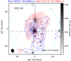 |
Fig. 7 Blueshifted and redshifted NH3 (1, 1) integrated-intensity contours overlaid on a 3.5 mm continuum. The blue and red contours are the blueshifted and redshifted velocity components, respectively. The blue contour levels start at − 3σ in steps of 3σ for NH3 (1, 1) with σ = 7.2 mJy beam−1km s−1, and the red ones with σ = 4.8 mJy beam−1km s−1. The black numbers indicate the positions of extracted NH2D cores. The synthesized beam sizes are indicated at the bottom-left corner. The dashed circle indicates the primary beam of the PdBI observations at 3.5 mm. The lines with arrows show the position-velocity cutting direction in Fig. 8. Other sources are presented in Fig. A.7. |
4.4 Excitation temperature
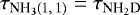
Figure 10 presents the relation between excitation temperatures Tex of NH2D and NH3 (1, 1) main groups for all NH2D cores. The excitation temperatures of the NH3 (1, 1) range from 7.0 to 13.0 K with a median width of 10.21 ± 0.28 K, while the excitation temperatures in the NH2D cores range from 3.9 to 10.0 Kwith a median width of 4.92 ± 0.09 K. Therefore, the NH2D have lower excitation temperature than the NH3 in the cores.
4.5 Kinetic temperature
Temperature in the dense core is vital in determining the chemical reaction rate of deuteration (Millar et al. 1989; Roberts & Millar 2000). Ammonia rotational lines NH3 (1, 1) and (2, 2) belong to the most useful tracers of the dense cores of molecular clouds, owing to the excitation and chemical properties (Ho & Townes 1983; Benson & Myers 1989; Tafalla et al. 2002; Friesen et al. 2009). They can remain gaseous in and nearby the cold, dense interior parts of starless and prestellar cores. They can thus be used as a precise tracer in probing the dust temperature (≲ 30 K) of dense and cold clumps, and in detecting the dynamical motions including outflow and rotation.
The kinetic temperature Tkin can be estimated from the rotational temperature Trot by using NH3 (1, 1) and (2, 2) transitions (Ott et al. 2011), assuming that the NH2D cores have the same temperature condition as the NH3 location. The calculation procedure of the kinetic temperature for each NH2D core is the same as the estimation for the continuum cores in Zhang et al. (2019a). The derived kinetic temperatures are listed in Table A.3 and presented in Figs. 11 and 12. It is quite evident that the NH2D cores have a colder condition than the continuum cores. Most NH2D cores have a temperature ranging from 13.5 to 18.5 K with a median width of 16.1 ± 0.5 K. Few NH2D cores have kinetic temperatures above 20 K. These cores with temperature above 20 K are always close to the central protostellar cores (see the right panel in Fig. 16), traced by strong 3.5 mm and 1.3 cm continuum. The statistics shows that the number of NH2D cores becomes small in a condition of relatively high temperature, for example these close to the central hot protostellar cores. It is possible that the NH2D excitation have been inhibited to some extent in such condition. Furthermore, the protostellar cores have a kinetic temperature ranging from around 10 to 40 K, and the median width is 22.1 ± 4.3 K, which is obviously higher than the kinetic temperature in the NH2D cores.
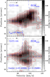 |
Fig. 8 Position–velocity diagrams of the main line of NH3 (1, 1) HfS along the position–velocity slice indicated with solid and dashed lines in Fig. 4 (see also Fig. 7). The arrows show the position–velocity cutting direction. Contour levels start at 3σ level and increase in steps of 3σ with σ = 3.3 mJy beam−1 for source G23.44. Blue dashed lines show a possible rotating toroids curve. The central mass, the central position, and the systemic velocity are indicated in the panel. Other sources are presented in Fig. A.8. |
4.6 Density and mass
We adopted the analysis routine described in Appendix of Pillai et al. (2007) to estimate the NH2D column density (see Table A.3). The derivation of NH3 column density (see Table A.3) follows the standard formulation in Bachiller et al. (1987). The H2 densities of continuum cores are discussed in Zhang et al. (2019a).
Due to the fact that there is no reliable abundance ratio available between NH2D and molecular hydrogen H2, we use the measured continuum flux within the Gaussian size of each NH2D core to derive a corresponding H2 column density and core mass (see Table A.3). If the continuum flux is lower than 3σ, we use the 3σ as an upper limit. The H2 volume density is estimated by assumingthe NH2D cores are in a spherical structure. The derived densities are listed in Table A.3. The derived H2 volume density for the NH2D cores ranges from 1.8 × 10⁵ to 2.4 × 106 cm−3 with a median width of (5.3 ± 1.4) × 105 cm−3, while that for the continuum cores ranges from 1.5 × 10⁵ to 4.6 × 106 cm−3 with a median width of (1.4 ± 0.1) × 106 cm−3. Therefore, the NH2D emission distributions are in a relatively less dense condition than the continuum cores.
The masses of NH2D cores are also estimated with a corresponding 3.5 mm continuum emission within the Gaussian size of each NH2D core. We calculate the mass of NH2D cores, using 3.5 mm dust opacity 0.002 cm2g−1 (Ossenkopf & Henning 1994), dust emissivity 1.7, and gas-to-dust mass ratio 100, and the derived kinetic temperature. The calculation processes have been shown in Sect. 4.4 of Zhang et al. (2019a). The derived parameters are listed in Table A.3. Figure 14 shows  -Reff distributions of all continuum and NH2D cores for comparisons. According to Kauffmann & Pillai (2010),[23.6pc] we also plot a threshold between high-mass and low-mass star candidates in Fig. 14, as it can be used to determine whether the NH2D cores are high-mass star formation candidates. The statistics shows that masses of the NH2D cores at a scale of Reff ≈ 0.05 pc range from 5.9 to 54.0 M⊙ with a median width of 13.8 ± 0.6 M⊙. This indicates that some of the NH2D cores may be intermediate- or high-mass candidates unless they further fragment.
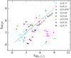 |
Fig. 9 Relation between optical depths τ of NH2D and NH3 (1, 1) main groups for all NH2D cores. The dashed line corresponds to |
 |
Fig. 10 Relation between excitation temperatures Tex
of NH2D and NH3
(1, 1) main groups for all NH2D cores. The dashed line corresponds to |
4.7 Deuterium fractionation
Deuterium fractionation is defined as ![$D_{\textrm{frac}} = N_{\textrm{NH}_2\textrm{D}}/N_{\textrm{NH}_3}={[\textrm{NH}_2\textrm{D}]/[\textrm{NH}_3]}$](/articles/aa/full_html/2020/06/aa36118-19/aa36118-19-eq7.png) (see calculations for NH3 and NH2D column densities in Sect. 4.6). We follow the analytical method of spectra NH3 and NH2D in Pillai et al. (2007) to estimate the deuterium fractionation for our detected NH2D cores. The derived results are listed in Table A.3. The deuterium fractionation range in 0.03≤ Dfrac ≤ 1.41 with a median width of 0.48 ± 0.01. Seven of these cores have Dfrac > 1.0.
(see calculations for NH3 and NH2D column densities in Sect. 4.6). We follow the analytical method of spectra NH3 and NH2D in Pillai et al. (2007) to estimate the deuterium fractionation for our detected NH2D cores. The derived results are listed in Table A.3. The deuterium fractionation range in 0.03≤ Dfrac ≤ 1.41 with a median width of 0.48 ± 0.01. Seven of these cores have Dfrac > 1.0.
4.8 Thermal and non-thermal velocities
In a gas at kinetic temperature Tkin, individual atoms will have random motions away from or towards the observer, leading to red- or blue-wards frequency shifts. The thermal σther and non-thermalσnth one-dimensional velocity dispersion in each source arising from a Maxwellian velocity distribution is:
 (1)
(1)
 (2)
(2)
where k is the Boltzmann constant,  is the molecular mass of the deuterated ammonia, and
  is the Gaussian line width FWHM of the NH2D.
The NH2D cores have quite narrow line widths with a median width of 0.98 ± 0.02 km s−1. Based on Eqs. (1) and (2), the thermal and non-thermal velocity dispersion have a median width of 0.09 ± 0.01 and 0.41 ± 0.01 km s−1, respectively (see also Fig. 11), indicating that only a very small part of thermal velocity contribute into the NH2D line width. Therefore, the non-thermal line broadening takes much higher weighting than the thermal velocity contribution. Comparing the line widths of the NH2D cores with the extracted 3.5 mm continuum cores in Zhang et al. (2019a), it is obvious that the 3.5 mm continuum cores have larger velocity dispersion than the NH2D cores within a similar source size. Therefore the NH2D cores are less turbulent than the 3.5 mm continuum cores.
4.9 Position-velocity diagrams
In Fig. 8, we present position–velocity diagrams in two different directions along the position-velocity slice indicated with the solid and dashed lines in Fig. 7, respectively. We also present possible Keplerian rotation curves in Fig. 8 via
 (3)
(3)
where vkep is the Keplerian velocity, G is the gravitational constant, Mcore is the continuum core mass, and r is the radiusfrom the central continuum peak position. In this work, the possible central mass within Keplerian orbit is up to 80 M⊙. The Pexistence of circumstellar disks (>30 M⊙) has remained elusive up to now. This observational result is likely to prove unsettling in the areas of theory and simulations. Therefore, the rotating structures are referred to as toroids (Beltrán & de Wit 2016), so as to distinguish them clearly from accretion disks in Keplerian rotation.
The diagrams in Figs. 8 and A.8 show what are obviously dynamical features of rotating toroids (Beltrán & de Wit 2016), such as G23.44, G23.97S, G25.38, and G25.71. We also present NH3 (1, 1) and (2, 2) lines at the peak position of 3.5 mm continuum distributions in Figs. 6 and A.6. The spectra show broadening line widths with somewhat blueshifted profiles, such as G23.44, G23.97S, G25.38, andG25.71. The characteristics shown in Figs. 6, A.6, 8, and A.8 indicate that such sources are dynamically active and that their envelopes (traced by NH3) may be rotating and infalling into the central dense cores (traced by 3.5 mm). It is likely that the central dense cores are boosting their massesby accretion to form a high-mass star in future. For the other four sources (G18.17, G18.21, G23.97N, and G23.98), however, their dynamical motions are relatively quiescent with a little narrower line width than the other four sources (see Fig. A.6). We also present their possible rotating toroids structure in Fig. A.8. It seems that the G18.21 shows some dynamical features of rotating toroids. Although the massive gas clumps (e.g., G23.97N and G23.98) do not have any embedded protostellar source down to Herschel far-infrared detection limits, the fragmentation and dynamical properties of the gas and dust are consistent with early collapse motion and clustered star formation, which was also argued by Beuther et al. (2013). Additionally, the central continuum cores in G18.17, G18.21, G23.97N, and G23.98 have relatively quiescent dynamical movements, but their large-scale gas distributions beyond the core size show a large velocity gradient (see Figs. A.4 and A.8).
The possible central mass within Keplerian orbit velocity for each source is roughly estimated and indicated in Fig. A.8. The sources G23.44, G23.97S, G25.38, and G25.71 have relatively large central mass with around 80 M⊙, while the masses in sources G18.17, G18.21, G23.97N, and G23.98 range from 10 to 30 M⊙. The evidence in Fig. A.8 may suggest that the accretion has started in prestellar core stage (e.g., G23.97N and G23.98), and the accretion rate continues to increase in protostellar stages (e.g., G23.44 and G23.97S).
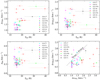 |
Fig. 11 Relation between velocity line widths Δv and kinetic temperatures Tkin for all NH2D cores. Lower right panel: the dashed line corresponds to |
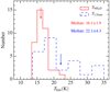 |
Fig. 12 Histogram of the kinetic temperatures Tkin estimated with lines NH3 (1, 1) and (2,2) for NH2D and 3.5 mm cores, respectively. The two downwards arrows show the corresponding median width. |
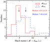 |
Fig. 13 Histogram for the ratio (Mach number |
4.10 Virial parameter
The virial theorem can be used to test whether one NH2D core is in a stable state. We assume a simple spherical fragment with a density distribution of ρ ∝ r−2, where r is the radius of spherical fragment. If ignoring magnetic fields, bulk motions, and external pressure of the gas, the virial mass of a fragment can be estimated with the formula (MacLaren et al. 1988; Evans 1999):
 (4)
(4)
where Reff is the source effective radius in pc and Δvnth is the non-thermal line width for NH2D main line (see also Eq. (2)). A similar derivation for virial mass can be found in Zhang et al. (2019a). However, one exception is that the velocity dispersion in this work was estimated with NH2D non-thermal velocity rather than NH3. The corresponding parameters are listed in Table A.3.
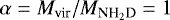
Comparing the virial mass Mvir with the NH2D core  , if the virial parameter
  , the dense source is gravitationally bound, potentially unstable, and to collapse; if αvir > 1, the source is not gravitationally bound, in a stable or expanding state. In Fig. 15, we show Mvir-
 distributions of all NH2D cores. The statistics shows that the virial parameters range from 0.11 to 3.48 with a median width of 0.55 ± 0.02. This indicates that the NH2D cores are mostly gravitationally bound.
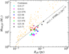 |
Fig. 14
|

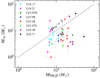 |
Fig. 15 Mvir- |

5 Discussion
5.1 Complex gas dynamics
NH3 (1, 1) is a good tracer of relatively dense gas and extended molecular clouds, and often used as dynamical tracer (e.g., Galván-Madrid et al. 2009; Zhang et al. 2014). To investigate the dynamical structure of the molecular clumps, we present the velocity distributions (moment 1) of NH3 (1, 1) in Fig. 4, which shows large velocity gradient and complicated distribution. Steep velocity gradient clearly exists in theeight molecular clumps, such as G18.17 and 23.97N in east-west direction, G23.44, G25.38, and G25.71 in north-south direction, and the other sources (G23.98 and G23.97S) having two velocity components crossing into together. The integrated-intensity maps in Fig. 7 show multiple emission peaks, even the blue- and red-shifted components present crossed distributions. It seems to be common to observe this dynamical phenomenon not only in the prestellar stage (e.g., G23.98) but in the protostellar stage as well (e.g., G23.97S). Csengeri et al. (2011a,b) explained this movement as a convergent flow. It is also likely that the molecular clumps are colliding with each other or simply overlapping in the plane of the sky but still physically separated in the third spatial dimension. In clumps G18.21, G23.98, G23.44, and G23.97S, the interaction regions of the possible convergent or colliding flows show relatively broad line width with no evidence of elevated gas temperatures (see Figs. 5 and A.5), while in clump G23.97S, we find a relatively high temperature as evidence of convergent or colliding flows (see the temperature distribution in Figs. 4 and D.10 of Zhang et al. 2019a). Furthermore, Figs. 8 and A.8 show possible rotating toroids signatures in all the eight sample. Thus, the convergent flow, the colliding flow, and the rotating toroids are coexistent in the clumps in a complicated way.
In Figs. 1 and A.1, the hyperfine lines of NH3 (1, 1) in some cores exhibit anomalous intensity ratios. For example, G18.17 Nos. 1, 2, and 6, G23.97N No. 1, G23.98 Nos. 1 and 4, G23.44 Nos. 1, 3, 5, 6, G23.97S No. 1, G25.38 No. 3, and G25.71 No. 1 show obviously stronger inner satellites on the blue side than on the red side, while G18.21 Nos. 1–9 have stronger outer satellites on the red side. The anomaly is only partially attributable to a non-LTE effect on the hyperfine transitions (Park 2001; Stutzki & Winnewisser 1985). It was suggested by Park (2001) that the hyperfine line intensity ratios could be tracing a systematic motion inside the dense cores. Park (2001) also found that expansion (outward motion) can strengthen the inner as well as outer satellite lines on the red (blue) side, while suppressing those (inward motion) on the other side, and that the line anomaly becomes prominent as the gas density increases. The anomalies further suggest complicated dynamical motions in the dense cores.
Since the detected NH2D lines are very narrow (<1.0 km s−1), and just cover several channels, it is really difficult to discuss the dynamics of the NH2D lines. We tried to use the blue- and red-shifted wings of the NH2D line to check whether one can find evidence of flow motions, but nothing was found. For the NH2D cores, the Mach number (the ratio of the non-thermal velocity dispersion σnth to the sound speed cs in Fig. 13) traced by NH2D has a median width of 4.83 ± 0.29, which is 1.5 times smaller than the Mach number traced by NH3. Therefore, the NH2D cores have a much more quiescent dynamics than the NH3 cores (see also the Mach number in Fig. 13). This suggests that the NH2D distributions have a very small velocity gradient. Figures 5 and A.5 also shows that the NH2D cores are often located at dynamically quiescent regions, relatively, for example in sources G23.44, G23.97S, and G25.38. In Fig. 7, the blue- and red-shifted spectral wing emission seems to be correlated with each 3.5 mm source separately, such as G18.17, G18.21, G23.44, and G25.71. It is likely that such individual sources have multiple velocity components. For clumps G23.97N, G23.97S, and G25.38, we find that the central continuum cores are located at the shearing positions of blue- and red-shifted components. It is likely that the central continuum cores are the power sources, which produce a large velocity dispersion of about 5 km s−1 probably derived by outflow motions.
5.2 Offset between NH2D cores and continuum peak
Seen from low-angular resolution of single-dish observations, deuterated species often have a good positional association with the cold cores in early stage. However, Roueff et al. (2005) found that deuterated species do not peak in protostars themselves, but at offset positions, and suggested that protostellar activity decreases deuteration built in the prestellar phase. Pillai et al. (2012) reported that the H2D+ peak is notassociated with either a dust continuum or N2 D+ peak. Friesen et al. (2014) revealed that there exists offset between H2D+ core and continuum peak positions, probably due to heating from undetected, young, low luminosity protostellar source or first hydrostatic core, or HD depletion in the cold center of the condensation in their opinion. As has also been argued by Pillai et al. (2011), the cold (< 20 K) and dense (> 106 cm−3) situations are two necessary conditions for producing a high NH2D abundance.
In Figs. 2 and 3, we overlaid NH2D integrated intensity contours on NH3 integrated intensity and 3.5 mm continuum images, respectively. Figure 16 displays the relation of the deuterium fractionation and kinetic temperature versus the projected offset distance to 3.5 mm continuum peak position for each NH2D core. We find that the NH2D peak positions are often not associated with either dust continuum or NH3 emission peak positions. Clumps G18.17, G18.21, G23.97N, and G23.98 have very weak infrared and millimeter emission, but strong and extended NH2D emission distributions. For clumps G23.44, G23.97S, and G25.38, the NH2D distributions are extended and surrounding the 3.5 mm continuum peak positions, and their minimum projected offset distances to the continuum peak nearby are 0.13, 0.12, and 0.17 pc, respectively (see also Fig. 16). In Fig. 2, for source G25.71, we only detected two weak NH2D emission. One core is located at the continuum peak position, another is far away from the continuum peak. Considering that G25.71 is an evolved source with an embedded protostellar core, it is really strange that the NH2D core (No. 1) has almost no projected offset from the peaked bright continuum core, which has a relatively high dust temperature of 28.8 ± 6.7 K. It may be possible that this NH2D core is just located in line of sight toward the continuum core. It is also likely that the 3.5 mm core in G25.71 has a very cold and thick NH2D envelope covering the hot dust insides. Generally, large projected offsets exist between the NH2D core and continuum peak positions, and the projected offsets are larger in evolved objects (e.g., G23.44, G23.97S, and G25.38) than those in the earlier evolutionary stages, (e.g., G23.97N and G23.98).
By measuring the kinetic temperatures of NH2D cores (see Fig. 12), we find a suitable condition for producing a high-level abundance of NH2D: dust temperature between 13.0 and 22.0 K (see also Sect. 5.3), and the corresponding column density derived from 3.5 mm continuum ranges from 4.0 × 10²² to 36.0 × 1022 cm−2. The NH2D distributions are also devoid of a bright infrared emission (see their infrared distributions in Zhang et al. 2019a), masers, and H II regions (see Figs. 2 and A.2). Based on the analysis above, we suggest that the NH2D emission close to the central bright continuum core (protostellar core) has been destroyed by an embedded young stellar object (YSO) due to its heating. The detected NH2D cores may be just the fragments of the cold and dense envelope associated with high-mass star-forming core insides. It is also very likely that the NH2D cores are massive starless seeds, some of which are possible to form future high-mass stars (see Fig. 14).
5.3 Very high deuterium fractionation
Deuterium fractionation is believed to be a fossil of cold chemistry in the early cold evolutionary phase (Parise et al. 2009; Pillai et al. 2012). Using single-dish observations, Pillai et al. (2007) found that 65% of the observed sample have strong NH2D emission with a high deuterium fractionation of 0.1 ≤ Dfrac ≤ 0.7. Toward G29.96e and G35.20w with interferometer, Pillai et al. (2011) obtained another deuterium fractionation of 0.06≤ Dfrac ≤ 0.37. Recently, Busquet et al. (2010) reported a high value of Dfrac ~ 0.8 in a pre-protostellar core close to high-mass star-forming region IRAS 20293+3952. By modeling the observed spectra, Harju et al. (2017) derived the fractionation ratios with Dfrac ~ 0.4.
High deuteration is mainly produced by two pathways: gas-phase ion-molecule chemistry and ice-grain surface chemistry (e.g., Rodgers & Charnley 2001; Millar 2002, 2003; Hatchell 2003; Roueff et al. 2005; Pillai et al. 2007). The root ion-neutral fractionation reaction is:
 (5)
(5)
which dominates at a temperature of <20 K, generally (e.g., Millar et al. 1989; Ceccarelli et al. 2014; Harju et al. 2017; De Simone et al. 2018). Neutral molecules like CO can destroy H2D+, thereby lowering the deuterium enhancement. Roberts & Millar (2000) suggested that at around 10 K, accretion of neutrals onto the dust grains, especially CO, leads to the formation of doubly deuterated molecules. Based on the above, we expect to see a correlation between the deuteration fractionation Dfrac and temperature Tkin. Figure 17 displays deuterium fractionation versus kinetic temperature for all the extracted NH2D cores. We find that the distribution between deuterium fractionation and kinetic temperature8 shows a number density peak at around Tkin = 16.1 K and Dfrac ~ 0.4, and the NH2D cores are mainly located at a temperature range of 13.0–22.0 K (see also the histogram of the kinetic temperatures in Fig. 12).
Figure 17 also displays a gas phase model predictions from Roueff et al. (2005) for comparison. Most of our sample have much higher deuterium fractionation than the model. Therefore, current models of gas phase reaction even under conditions of high depletion are not capable of explaining the high fractionation observed in this work. The gas-grain chemical reactions are expected to explain the production of the high deuterium fractionation. However, few corresponding gas-grain chemical models are currently available. Additionally, deuterium fractionation Dfrac > 1.0 warrant closer scrutiny. We attribute such anomalous values to missing short spacing information in our data. However, comparing with single-dish observations in Pillai et al. (2007), the deuterium fractionation has been up to 0.7 in clump G18.17. Therefore, it is reasonable for the three higher deuterium fractionations (e.g., Dfrac ~ 1.06 for NH2D core No. 1, Dfrac ~ 1.37 for No. 4, and Dfrac ~ 1.26 for No. 6 in clump G18.17) with higher spatial resolution from interferometer observations.
As seen from the diagram between the deuterium fractionation and kinetic temperature in Fig. 17, these data points are just scattering from 13.0 to 22.0 K, and the median value is around 16.1 K. Therefore, the suitable condition for NH2D production mainly ranges from 13.0 to 22.0 K, and the deuterium fractionations will reach up to the maximum at 16.1 K. For these higher than 22.0 K, the activity of NH2D production is likely inhibited, and maybe they have been dissociated (e.g., Rodgers & Charnley 2001; Millar 2002, 2003; Roueff et al. 2005). When it is less than 13.0 K, it is possible that NH2D also tends to be frozen out onto dust grain (Brown & Millar 1989a,b; Fedoseev et al. 2015a). However, we also should not ignore that the tracer of kinetic temperature, NH3, may have been seriously frozen onto the dust grain before NH2D has (Fedoseev et al. 2015b). Therefore, it may be not suitable to use NH3 and NH2D as tracers to study dense gas at a temperature condition of Tkin < 13.0 K.
In Fig. 16, we plot the relation in the deuterium fractionation and kinetic temperature versus the projected offset distance to 3.5 mm continuum peak position for each NH2D core. We find that the NH2D cores are located within a projected radius region between 0.02 and 0.5 pc. It seems that the deuterium fractionation or kinetic temperature distribution does not vary significantly with the changes of the projected offset distances between between 0.02 and 0.5 pc. In other projected offset areas, we detected few NH2D cores. This diverges from what has been suggested by Friesen et al. (2018). It is possible that the cold dust envelopes are extremely thick enough, leading to that most of heating from the central hot source has been cooled down by the envelopes.
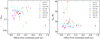 |
Fig. 16 Deuterium fractionation Dfrac and kinetic temperature Tkin versus the projected offset distance to 3.5 mm continuum peak position for each NH2D core. |
5.4 Deuteration is a poor evolutionary indicator of star formation in evolved stage
Many previous works (e.g., Fontani et al. 2011; Brünken et al. 2014; Ceccarelli et al. 2014) argued that the deuteration can be used as an evolutionary indicator of star formation in a wide range of evolutionary stages, for example, from high-mass starless core candidates (HMSCs) to high-mass protostellar objects (HMPOs) and ultracompact (UC) H II regions (for a definition of these stages see e.g. Beuther et al. 2007). Busquet et al. (2010) found that in a high-mass star-forming region (harbouring an UC H II region), the deuterium fractionation increases until the onset of star formation and decreases afterwards. The method is to check the changes of deuterium abundance in different evolutionary stages. Since the evolved sources often have high dust temperature (> 30 K), the growth of deuterium fractionation will be inhibited easily (see Sect. 5.3). So, what is the nature of the deuterium emission that still can be detected even in evolved objects (e.g., HMPOs and UC H II regions)? We think that previous observationsmainly focused on using single-dish telescopes or interferometers with relatively low spatial resolution. They were not able to resolve the distributions of deuterium species from central bright sources, for example HMSCs, HMPOs, and UC H II regions.
In our PdBI NH2D observations, we find that thepositions detected with NH2D emission areoften offset far away from the protostellar cores, traced by bright 3.5 mm and 1.3 cm continuum (see Sect. 5.2). Fontani et al. (2006) proposed two scenarios: in the first one, the cold gas is distributed in an external shell not yet heated up by the high-mass protostellar object, a remnant of the parental massive starless core, due to heavily thick envelope of high-mass star formation; in the second one, the cold gas is located in cold and dense cores close to the high-mass protostellar cores but not associated with them. We also argue that the NH2D that we detected does not emit from the evolved objects indeed. Considering that the high-mass stars often form in clusters (Tutukov 1978; Kurtz et al. 2000), the detected NH2D cores may be just some cold and dense fragments of the neighbouring evolved objects. Basically, the detected NH2D cores belongto prestellar or starless objects (see Sect. 5.2). Therefore, these deuterium production should have few correlation with the HMPOs and UC H II regions.
In this work, we do not see much discrepancy (see Fig. 17) in deuteration fractionation between the early evolutionary stage of sources (e.g., G18.17, G18.21) and the evolved objects (e.g., G23.44, G23.97S). This further suggests that the habitat conditions where NH2D remains gaseous have no direct correlation with different evolutionary stages but, rather, they depend mainly on the temperature conditions between 13.0 and 22.0 K and the density condition of around 5.3 × 105 cm−3. The HMPOs and UC H II regions often have high dust temperature of > 30 K, which is too high for significant deuterium fractionation. It is for this reason that, in principle, the observed cold and dense gas responsible for the NH2D emission may be not associated with the high-mass evolved objects. Therefore, NH2D is a poor evolutionary indicator of high-mass star formation in evolved stages, but a useful tracer in the starless and prestellar cores.
 |
Fig. 17 Deuterium fractionation Dfrac versus kinetic temperature Tkin for all NH2D cores. The solid line is the latest gas phase model predictions from Roueff et al. (2005). The contours show the number density distribution of the cores. The data points with error bars are derived from this work. |
6 Summary
At the early stages (e.g., prestellar or starless core stages) of star formation, most species tend to be frozen out onto dust grains, except deuterium molecules and ions. Using the PdBI and the VLA, we presented o-NH2D 111 –101 and NH3 (1, 1), (2, 2) observations in eight massive precluster protocluster clumps including G18.17, G18.21, G23.97N, G23.98, G23.44, G23.97S, G25.38, and G25.71. We used 3D GAUSSCLUMPS to extract NH2D cores and provided a statistical view of their deuterium chemistry.
We detected seven instances of extremely high deuterium fractionation of 1.0 ≤ Dfrac ≤ 1.41 in the NH2D cores. Current gas phase models have difficulty for explaining the high fractionation observed in this work. The gas-grain chemical reactions are needed to explain the production of the high deuterium fractionation. In addition, we found that the distribution between deuterium fractionation and kinetic temperature shows a number density peak at around Tkin = 16.1 K, and the NH2D cores are mainly located at a temperature range of 13.0–22.0 K. The 3.5 mm continuum cores have a kinetic temperature with the median width of 22.1 ± 4.3 K, which is obviously higher than the temperature in NH2D cores. This suggests that the high deuterium fractionation strongly depends on the temperature condition.
We found that the NH2D emission is often not associated with either a dust continuum or NH3 emission peak positions. For the protocluster clumps G23.44, G23.97S, and G25.38, the NH2D distributions are extended and surrounding the 3.5 mm continuum peak positions, and their minimum projected offset distances to the continuum peak nearby are 0.13, 0.12, and 0.17 pc, respectively. We also found that large projected offsets exist between the NH2D core and continuum peak positions, and the projected offsets are larger in the more evolved objects, for example G23.44, G23.97S, and G25.38 in protostellar core stage than those in the earlier evolutionary stages, for example G23.97N and G23.98 in prestellar core stage.
We found that the NH3 and NH2D are often optically thick in these clumps with a median width of 4.05 ± 0.04 and 3.22 ± 0.10, respectively. The masses of the NH2D cores at a scale of Reff ≈ 0.05 pc range from 5.9 to 54.0 M⊙ with a median width of 13.8 ± 0.6 M⊙. The NH2D cores are mostly gravitationally bound (αvir < 1), are likely prestellar or starless, and can potentially form intermediate-mass or high-mass stars in future.
The derived volume density of the NH2D cores is between 1.8 × 10⁵ and 2.4 × 106 cm−3 with a median width of (5.3 ± 1.4) × 105 cm−3, while that ofcontinuum cores ranges from 1.5 × 10⁵ to 4.6 × 106 cm−3 with a median width of (1.4 ± 0.1) × 106 cm−3. Therefore, the NH2D distributions are in a relatively less dense condition than the continuum cores.
The detected NH2D line widths are very narrow with a median width of 0.98 ± 0.02 km s−1, where the thermal and non-thermal velocity dispersion have a median width of 0.09 ± 0.01 and 0.41 ± 0.01 km s−1 in the NH2D cores, respectively. Therefore, non-thermal motions still contribute significantly to the line width of NH2D.
We found that the detected NH2D cores belong to prestellar or starless object stages. The association between the NH2D cores and the evolved objects is not significant. The remaining of NH2D mainly depends on the suitable temperature of around 13.0 to 22.0 K and the density of ~5.3 × 105 cm−3. Therefore, we suggest that the NH2D is a useful tracer in prestellar or starless cores, but cannot be used as a precise indicator in other evolved stages.
Using NH3 (1, 1) as a dynamical tracer, we found evidence of very complicated dynamical movement in all the eight clumps, either outflow and rotation or convergent flow and colliding each other, not only in earlier stage of clumps but also in evolved objects. The velocity signatures that indicate to rotating toroids are also identified. The sample partly present obvious dynamical characteristic of rotating toroids, suggesting that accretion has started and continues to increase gradually from the prestellar core stage (e.g., G23.97N and G23.98) to the protostellar stage (e.g., G23.44 and G23.97S). Additionally, the central continuum cores in G18.17, G18.21, G23.97N, and G23.98 have relatively quiescent dynamical movements, but their large-scale gas distributions beyond the core size show a large velocity gradient.
Acknowledgements
We thank the anonymous referees for constructive comments that improved the manuscript. This work is supported by the National Natural Science Foundation of China No. 11703040, and the National Key Basic Research Program of China (973 Program) No. 2015CB857101. C.-P.Z. acknowledges support by the NAOC Nebula Talents Program and the China Scholarship Council in Germany as a postdoctoral researcher (No. 201704910137).
Appendix A Additional tables and figures
Coordinates of infrared sources, H II regions, and masers.
Parameters of the identified NH2D cores: position, velocity, line width, brightness temperature, optical depth and excitation temperature.
Parameters of the identified NH2D cores: size, temperature, mass, density, and deuterium fractionation.
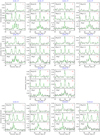 |
Fig. A.1 Spectra NH2D, NH3 (1, 1) and (2,2) overlaid with their HfS fits for all NH2D cores (see Table A.2). The spectra are derived by averaging the lines within each NH2D core scale. |
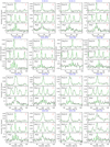 |
Fig. A.1 continued. |
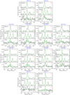 |
Fig. A.1 continued. |
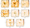 |
Fig. A.2 NH2D integrated-intensity contours overlaid on a 3.5 mm continuum with velocity range covering all the six HfS lines. The contour levels start at − 3σ in steps of 3σ for NH2D with σ(a)-(h) = 60.4, 60.9, 51.1, 53.2, 33.6, 23.4, 26.9, 50.4 mJy beam−1km s−1. The green ellipses with red numbers indicate the positions of extracted NH2D cores. The symbols “▴”, “■”, and “⋆” indicate thepositions of masers, H II regions, and infrared sources, respectively. The synthesized beam sizes of each subfigure are indicated at the bottom-left corner. The dashed circle indicates the primary beam of the PdBI observations at 3.5 mm. |
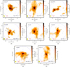 |
Fig. A.3 NH2D integrated-intensity contours overlaid on an NH3 (1, 1) integrated-intensity image with velocity range covering all the six HfS lines. The contour levels start at − 3σ in steps of 3σ for NH2D with σ(a)-(h) = 60.4, 60.9, 51.1, 53.2, 33.6, 23.4, 26.9, 50.4 mJy beam−1km s−1. The red numbers indicate the positions of extracted NH2D cores. The synthesized beam sizes of each subfigure are indicated at the bottom-left corner. The dashed circle indicates the primary beam of the PdBI observations at 3.5 mm. |
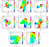 |
Fig. A.4 Velocity distribution (moment 1) of NH3 (1, 1) line overlaid with integrated-intensity contours (moment 0) of NH2D line with velocity range covering all the six HfS lines. The contour levels start at − 3σ in steps of 3σ for NH2D with σ(a)-(h) = 60.3, 60.9, 51.1, 53.2, 84.1, 48.3, 49.0, 50.4 mJy beam−1km s−1. The synthesized beam sizes of each subfigure are indicated at the bottom-left corner. The dashed circle indicates the primary beam of the PdBI observations at 3.5 mm. The lines with arrows show the cutting direction in Fig. A.8. |
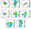 |
Fig. A.5 Line width distribution (moment 2) of NH3 (1, 1) line overlaid with integrated-intensity contours (moment 0) of NH2D line with velocity range covering all the six HfS lines. The contour levels start at − 3σ in steps of 3σ for NH2D with σ(a)-(h) = 60.3, 60.9, 51.1, 53.2, 84.1, 48.3, 49.0, 50.4 mJy beam−1km s−1. The synthesized beam sizes of each subfigure are indicated at the bottom-left corner. The dashed circle indicates the primary beam of the PdBI observations at 3.5 mm. |
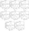 |
Fig. A.6 Spectra of NH3 (1, 1) and (2, 2) obtained toward a single and the brightest pixel at 3.5 mm continuum. The coordinates of the spectra are indicated at each corresponding lower panel of Fig. A.8. |
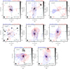 |
Fig. A.7 Blueshifted and redshifted NH3 (1, 1) integrated-intensity contours overlaid on a 3.5 mm continuum. The blue and red contours are the blueshifted and redshifted velocity components, respectively. The blue contour levels start at − 3σ in steps of 3σ for NH3 (1, 1) with σ(a)-(h) = 5.0, 6.8, 3.2, 4.9, 7.2, 5.5, 5.3, 5.6 mJy beam−1km s−1, and the red ones with σ(a)-(h) = 5.7, 9.1, 4.5, 3.7, 4.8, 4.8, 5.2, 5.0 mJy beam−1km s−1. The black numbers indicate the positions of extracted NH2D cores. The synthesized beam sizes of each subfigure are indicated at the bottom-left corner. The dashed circle indicates the primary beam of the PdBI observations at 3.5 mm. The lines with arrows show the position-velocity cutting direction in Fig. A.8. |
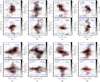 |
Fig. A.8 Position–velocity diagrams of the main line of NH3 (1, 1) HfS along the position-velocity slice indicated with solid and dashed lines in Fig. A.4 (see also Fig. A.7). The arrows show the position–velocity cutting direction. Contour levels start at 3σ level and increase in steps of 3σ with σ(a)-(h) = ~3.4, ~4.4, ~2.5, ~2.5, ~3.3, ~3.4, ~2.7, and ~2.8 mJy beam−1 for source G18.17, G18.21,..., G25.71, respectively. Blue dashed lines show a possible rotating toroids curve. The central mass, the central position, and the systemic velocity are indicated in each subfigure. |
References
- Ai, M., Zhu, M., Xiao, L., & Su, H.-Q. 2013, Res. Astron. Astrophys., 13, 935 [NASA ADS] [CrossRef] [Google Scholar]
- Anderson, L. D., & Bania, T. M. 2009, ApJ, 690, 706 [NASA ADS] [CrossRef] [Google Scholar]
- Bachiller, R., Guilloteau, S., & Kahane, C. 1987, A&A, 173, 324 [NASA ADS] [Google Scholar]
- Beltrán, M. T., & de Wit, W. J. 2016, A&ARv, 24, 6 [NASA ADS] [CrossRef] [Google Scholar]
- Benson, P. J., & Myers, P. C. 1989, ApJS, 71, 89 [NASA ADS] [CrossRef] [Google Scholar]
- Bergin, E. A., & Tafalla, M. 2007, ARA&A, 45, 339 [NASA ADS] [CrossRef] [Google Scholar]
- Beuther, H., Churchwell, E. B., McKee, C. F., & Tan, J. C. 2007, Protostars and Planets V (Tucson, AX: University of Arizona Press), 165 [Google Scholar]
- Beuther, H., Linz, H., Tackenberg, J., et al. 2013, A&A, 553, A115 [NASA ADS] [CrossRef] [EDP Sciences] [Google Scholar]
- Breen, S. L., Fuller, G. A., Caswell, J. L., et al. 2015, MNRAS, 450, 4109 [NASA ADS] [CrossRef] [Google Scholar]
- Brown, P. D., & Millar, T. J. 1989a, MNRAS, 240, 25 [NASA ADS] [CrossRef] [EDP Sciences] [Google Scholar]
- Brown, P. D., & Millar, T. J. 1989b, MNRAS, 237, 661 [NASA ADS] [Google Scholar]
- Brünken, S., Sipilä, O., Chambers, E. T., et al. 2014, Nature, 516, 219 [NASA ADS] [CrossRef] [PubMed] [Google Scholar]
- Brunthaler, A., Reid, M. J., Menten, K. M., et al. 2009, ApJ, 693, 424 [NASA ADS] [CrossRef] [Google Scholar]
- Busquet, G., Palau, A., Estalella, R., et al. 2010, A&A, 517, L6 [NASA ADS] [CrossRef] [EDP Sciences] [Google Scholar]
- Ceccarelli, C., Caselli, P., Bockelée-Morvan, D., et al. 2014, Protostars and Planets VI (Tucson, AZ: University of Arizona Press), 859 [Google Scholar]
- Churchwell, E. 2002, ARA&A, 40, 27 [Google Scholar]
- Crapsi, A., Caselli, P., Walmsley, C. M., et al. 2005, ApJ, 619, 379 [Google Scholar]
- Csengeri, T., Bontemps, S., Schneider, N., Motte, F., & Dib, S. 2011a, A&A, 527, A135 [NASA ADS] [CrossRef] [EDP Sciences] [Google Scholar]
- Csengeri, T., Bontemps, S., Schneider, N., et al. 2011b, ApJ, 740, L5 [NASA ADS] [CrossRef] [Google Scholar]
- Cyganowski, C. J., Whitney, B. A., Holden, E., et al. 2008, AJ, 136, 2391 [NASA ADS] [CrossRef] [Google Scholar]
- Daniel, F., Rist, C., Faure, A., et al. 2016a, MNRAS, 457, 1535 [NASA ADS] [CrossRef] [EDP Sciences] [Google Scholar]
- Daniel, F., Coudert, L. H., Punanova, A., et al. 2016b, A&A, 586, L4 [NASA ADS] [CrossRef] [EDP Sciences] [Google Scholar]
- De Simone, M., Fontani, F., Codella, C., et al. 2018, MNRAS, 476, 1982 [NASA ADS] [CrossRef] [Google Scholar]
- de Villiers, H. M., Chrysostomou, A., Thompson, M. A., et al. 2014, MNRAS, 444, 566 [NASA ADS] [CrossRef] [Google Scholar]
- Evans, II, N. J. 1999, ARA&A, 37, 311 [NASA ADS] [CrossRef] [Google Scholar]
- Fedoseev, G., Ioppolo, S., & Linnartz, H. 2015a, MNRAS, 446, 449 [NASA ADS] [CrossRef] [Google Scholar]
- Fedoseev, G., Ioppolo, S., Zhao, D., Lamberts, T., & Linnartz, H. 2015b, MNRAS, 446, 439 [NASA ADS] [CrossRef] [Google Scholar]
- Flower, D. R., Pineau Des Forêts, G., & Walmsley, C. M. 2006, A&A, 449, 621 [NASA ADS] [CrossRef] [EDP Sciences] [Google Scholar]
- Fontani, F., Caselli, P., Crapsi, A., et al. 2006, A&A, 460, 709 [NASA ADS] [CrossRef] [EDP Sciences] [Google Scholar]
- Fontani, F., Palau, A., Caselli, P., et al. 2011, A&A, 529, L7 [NASA ADS] [CrossRef] [EDP Sciences] [Google Scholar]
- Friesen, R. K., Di Francesco, J., Shirley, Y. L., & Myers, P. C. 2009, ApJ, 697, 1457 [NASA ADS] [CrossRef] [Google Scholar]
- Friesen, R. K., Di Francesco, J., Bourke, T. L., et al. 2014, ApJ, 797, 27 [NASA ADS] [CrossRef] [Google Scholar]
- Friesen, R. K., Beltrán, M. T., Caselli, P., & Garrod, R. T. 2018, ASP Conf. Ser., 517, 381 [NASA ADS] [Google Scholar]
- Fukui, Y., Torii, K., Hattori, Y., et al. 2018, ApJ, 859, 166 [NASA ADS] [CrossRef] [Google Scholar]
- Fuller, G. A., Williams, S. J., & Sridharan, T. K. 2005, A&A, 442, 949 [NASA ADS] [CrossRef] [EDP Sciences] [Google Scholar]
- Galván-Madrid, R., Keto, E., Zhang, Q., et al. 2009, ApJ, 706, 1036 [NASA ADS] [CrossRef] [Google Scholar]
- Gong, Y., Fang, M., Mao, R., et al. 2017, ApJ, 835, L14 [NASA ADS] [CrossRef] [Google Scholar]
- Green, J. A., Caswell, J. L., Fuller, G. A., et al. 2010, MNRAS, 409, 913 [NASA ADS] [CrossRef] [Google Scholar]
- Harju, J., Daniel, F., Sipilä, O., et al. 2017, A&A, 600, A61 [NASA ADS] [CrossRef] [EDP Sciences] [Google Scholar]
- Hatchell, J. 2003, A&A, 403, L25 [NASA ADS] [CrossRef] [EDP Sciences] [Google Scholar]
- Ho, P. T. P. 1977, PhD thesis, Massachusetts Institute of Technology, USA [Google Scholar]
- Ho, P. T. P., & Townes, C. H. 1983, ARA&A, 21, 239 [NASA ADS] [CrossRef] [Google Scholar]
- Kauffmann, J., & Pillai, T. 2010, ApJ, 723, L7 [NASA ADS] [CrossRef] [Google Scholar]
- Keto, E. 2007, ApJ, 666, 976 [NASA ADS] [CrossRef] [Google Scholar]
- Kramer, C., Stutzki, J., & Winnewisser, G. 1996, A&A, 307, 915 [Google Scholar]
- Kramer, C., Stutzki, J., Rohrig, R., & Corneliussen, U. 1998, A&A, 329, 249 [NASA ADS] [Google Scholar]
- Kukolich, S. G. 1967, Phys. Rev., 156, 83 [NASA ADS] [CrossRef] [Google Scholar]
- Kurtz, S., Cesaroni, R., Churchwell, E., Hofner, P., & Walmsley, C. M. 2000, Protostars and Planets IV (Tucson, AZ: University of Arizona Press), 299 [Google Scholar]
- Liu, T., Wu, Y., Zhang, Q., et al. 2011, ApJ, 728, 91 [NASA ADS] [CrossRef] [Google Scholar]
- Lockman, F. J. 1989, ApJS, 71, 469 [NASA ADS] [CrossRef] [Google Scholar]
- Lu, X., Zhang, Q., Liu, H. B., et al. 2018, ApJ, 855, 9 [NASA ADS] [CrossRef] [Google Scholar]
- MacLaren, I., Richardson, K. M., & Wolfendale, A. W. 1988, ApJ, 333, 821 [NASA ADS] [CrossRef] [Google Scholar]
- Millar, T. J. 2002, Planet. Space Sci., 50, 1189 [CrossRef] [Google Scholar]
- Millar, T. J. 2003, Space Sci. Rev., 106, 73 [NASA ADS] [CrossRef] [Google Scholar]
- Millar, T. J., Bennett, A., & Herbst, E. 1989, ApJ, 340, 906 [NASA ADS] [CrossRef] [Google Scholar]
- Motte, F., Bontemps, S., Schilke, P., et al. 2007, A&A, 476, 1243 [NASA ADS] [CrossRef] [EDP Sciences] [Google Scholar]
- Müller, H. S. P., Schlöder, F., Stutzki, J., & Winnewisser, G. 2005, J. Mol. Struct., 742, 215 [NASA ADS] [CrossRef] [Google Scholar]
- Oliveira, C. M., Hébrard, G., Howk, J. C., et al. 2003, ApJ, 587, 235 [NASA ADS] [CrossRef] [Google Scholar]
- Ossenkopf, V., & Henning, T. 1994, A&A, 291, 943 [NASA ADS] [Google Scholar]
- Ott, J., Henkel, C., Braatz, J. A., & Weiß, A. 2011, ApJ, 742, 95 [NASA ADS] [CrossRef] [Google Scholar]
- Pagani, L., Daniel, F., & Dubernet, M.-L. 2009, A&A, 494, 719 [NASA ADS] [CrossRef] [EDP Sciences] [Google Scholar]
- Parise, B., Leurini, S., Schilke, P., et al. 2009, A&A, 508, 737 [NASA ADS] [CrossRef] [EDP Sciences] [Google Scholar]
- Park, Y. S. 2001, A&A, 376, 348 [NASA ADS] [CrossRef] [EDP Sciences] [Google Scholar]
- Peretto, N., Fuller, G. A., André, P., et al. 2014, A&A, 561, A83 [NASA ADS] [CrossRef] [EDP Sciences] [Google Scholar]
- Pillai, T., Wyrowski, F., Hatchell, J., Gibb, A. G., & Thompson, M. A. 2007, A&A, 467, 207 [NASA ADS] [CrossRef] [EDP Sciences] [Google Scholar]
- Pillai, T., Kauffmann, J., Wyrowski, F., et al. 2011, A&A, 530, A118 [NASA ADS] [CrossRef] [EDP Sciences] [Google Scholar]
- Pillai, T., Caselli, P., Kauffmann, J., et al. 2012, ApJ, 751, 135 [NASA ADS] [CrossRef] [Google Scholar]
- Reid, M. J., Menten, K. M., Zheng, X. W., et al. 2009, ApJ, 700, 137 [NASA ADS] [CrossRef] [Google Scholar]
- Ren, J. Z., Liu, T., Wu, Y., & Li, L. 2011, MNRAS, 415, L49 [NASA ADS] [CrossRef] [Google Scholar]
- Roberts, H., & Millar, T. J. 2000, A&A, 361, 388 [NASA ADS] [Google Scholar]
- Rodgers, S. D., & Charnley, S. B. 2001, ApJ, 553, 613 [NASA ADS] [CrossRef] [EDP Sciences] [Google Scholar]
- Roueff, E., Lis, D. C., van der Tak, F. F. S., Gerin, M., & Goldsmith, P. F. 2005, A&A, 438, 585 [NASA ADS] [CrossRef] [EDP Sciences] [Google Scholar]
- Shu, F. H., Adams, F. C., & Lizano, S. 1987, ARA&A, 25, 23 [Google Scholar]
- Sipilä, O., Caselli, P., & Harju, J. 2015a, A&A, 578, A55 [NASA ADS] [CrossRef] [EDP Sciences] [Google Scholar]
- Sipilä, O., Harju, J., Caselli, P., & Schlemmer, S. 2015b, A&A, 581, A122 [NASA ADS] [CrossRef] [EDP Sciences] [Google Scholar]
- Stutzki, J., & Guesten, R. 1990, ApJ, 356, 513 [NASA ADS] [CrossRef] [Google Scholar]
- Stutzki, J., & Winnewisser, G. 1985, A&A, 144, 13 [NASA ADS] [Google Scholar]
- Tafalla, M., Myers, P. C., Caselli, P., Walmsley, C. M., & Comito, C. 2002, ApJ, 569, 815 [NASA ADS] [CrossRef] [Google Scholar]
- Tiné, S., Roueff, E., Falgarone, E., Gerin, M., & Pineau des Forêts, G. 2000, A&A, 356, 1039 [NASA ADS] [Google Scholar]
- Tutukov, A. V. 1978, A&A, 70, 57 [NASA ADS] [Google Scholar]
- Urquhart, J. S., Thompson, M. A., Moore, T. J. T., et al. 2013, MNRAS, 435, 400 [NASA ADS] [CrossRef] [Google Scholar]
- Walmsley, C. M., Flower, D. R., & Pineau des Forêts, G. 2004, A&A, 418, 1035 [NASA ADS] [CrossRef] [EDP Sciences] [Google Scholar]
- Wienen, M., Wyrowski, F., Schuller, F., et al. 2012, A&A, 544, A146 [NASA ADS] [CrossRef] [EDP Sciences] [Google Scholar]
- Yuan, J., Li, J.-Z., Wu, Y., et al. 2018, ApJ, 852, 12 [NASA ADS] [CrossRef] [Google Scholar]
- Zhang, C.-P., Wang, J.-J., & Xu, J.-L. 2013, A&A, 550, A117 [NASA ADS] [CrossRef] [EDP Sciences] [Google Scholar]
- Zhang, C.-P., Wang, J.-J., Xu, J.-L., Wyrowski, F., & Menten, K. M. 2014, ApJ, 784, 107 [NASA ADS] [CrossRef] [Google Scholar]
- Zhang, C.-P., Li, G.-X., Wyrowski, F., et al. 2016, A&A, 585, A117 [NASA ADS] [CrossRef] [EDP Sciences] [Google Scholar]
- Zhang, C.-P., Liu, T., Yuan, J., et al. 2018, ApJS, 236, 49 [NASA ADS] [CrossRef] [Google Scholar]
- Zhang, C.-P., Csengeri, T., Wyrowski, F., et al. 2019a, A&A, 627, A85 [NASA ADS] [CrossRef] [EDP Sciences] [Google Scholar]
- Zhang, C.-P., Li, G.-X., Zhou, C., Yuan, L., & Zhu, M. 2019b, A&A, 631, A110 [NASA ADS] [CrossRef] [EDP Sciences] [Google Scholar]
- Zhou, P., Chen, Y., Safi-Harb, S., et al. 2016a, ApJ, 831, 192 [Google Scholar]
- Zhou, P., Chen, Y., Zhang, Z.-Y., et al. 2016b, ApJ, 826, 34 [NASA ADS] [CrossRef] [Google Scholar]
- Zhu, M., Davis, C. J., Wu, Y., et al. 2011, ApJ, 739, 53 [CrossRef] [Google Scholar]
- Zinnecker, H., & Yorke, H. W. 2007, ARA&A, 45, 481 [NASA ADS] [CrossRef] [Google Scholar]
In Fig. A.1, some main HfS lines in NH2D show multi-velocity components (e.g., G18.17 No. 2, G18.17 No. 5, and G23.44 Nos, 1, 3, 7, 8). For comparison, we only consider the strongest velocity components associated with the corresponding NH3 line. This could bring some error into the line width.
However, we have to note that the NH2D excitation temperature is smaller than the NH3 excitation temperature (see also Fig. 10). Then by using the NH3 temperatures the NH2D column density will be overestimated and in turn the deuterium fractionation.
All Tables
Parameters of the identified NH2D cores: position, velocity, line width, brightness temperature, optical depth and excitation temperature.
Parameters of the identified NH2D cores: size, temperature, mass, density, and deuterium fractionation.
All Figures
|
Fig. 1 Spectra NH2D, NH3 (1, 1) and (2,2) overlaid with their HfS fits for the first two NH2D cores (see Table A.2). The spectra are derived by averaging the lines within each NH2D core scale. Other sources and spectra are presented in Fig A.1. |
| In the text | |
|
Fig. 2 NH2D integrated-intensity contours overlaid on a 3.5 mm continuum with velocity range covering all the six HfS lines. The contour levels start at − 3σ in steps of 3σ for NH2D with σ = 33.6 mJy beam−1km s−1. The green ellipses with red numbers indicate the positions of extracted NH2D cores. The symbols “▴”, “■”, and “⋆” indicate the positions of masers, H II regions, and infrared sources, respectively. The synthesized beam sizes are indicated at the bottom-left corner. The dashed circle indicates the primary beam of the PdBI observations at 3.5 mm. Other sources are presented in Fig. A.2. |
| In the text | |
|
Fig. 3 NH2D integrated-intensity contours overlaid on an NH3 (1, 1) integrated-intensity image with velocity range covering all the six HfS lines. The contour levels start at − 3σ in steps of 3σ for NH2D with σ = 33.6 mJy beam−1km s−1. The synthesized beam sizes are indicated at the bottom-left corner. The dashed circle indicates the primary beam of the PdBI observations at 3.5 mm. Other sources are presented in Fig. A.3. |
| In the text | |
|
Fig. 4 Velocity distribution (moment 1) of NH3 (1, 1) line overlaid with integrated-intensity contours (moment 0) of NH2D line with velocity range covering all the six HfS lines. The contour levels start at − 3σ in steps of 3σ for NH2D with σ = 84.1 mJy beam−1km s−1. The synthesized beam sizes are indicated at the bottom-left corner. The dashed circle indicates the primary beam of the PdBI observations at 3.5 mm. The lines with arrows show the position-velocity cutting direction in Fig. 8. Other sources are presented in Fig. A.4. |
| In the text | |
|
Fig. 5 Line width distribution (moment 2) of NH3 (1, 1) line overlaid with integrated-intensity contours (moment 0) of NH2D line with velocity range covering all the six HfS lines. The contour levels start at − 3σ in steps of 3σ for NH2D with σ = 84.1 mJy beam−1km s−1. The synthesized beam sizes are indicated at the bottom-left corner. The dashed circle indicates the primary beam of the PdBI observations at 3.5 mm. Other sources are presented in Fig. A.5. |
| In the text | |
|
Fig. 6 Spectra NH3 (1, 1) and (2, 2) obtained toward a single and the brightest pixel at 3.5 mm continuum. The coordinates of the spectra are indicated at the lower panel of Fig. 8. Other sources are presented in Fig. A.6. |
| In the text | |
|
Fig. 7 Blueshifted and redshifted NH3 (1, 1) integrated-intensity contours overlaid on a 3.5 mm continuum. The blue and red contours are the blueshifted and redshifted velocity components, respectively. The blue contour levels start at − 3σ in steps of 3σ for NH3 (1, 1) with σ = 7.2 mJy beam−1km s−1, and the red ones with σ = 4.8 mJy beam−1km s−1. The black numbers indicate the positions of extracted NH2D cores. The synthesized beam sizes are indicated at the bottom-left corner. The dashed circle indicates the primary beam of the PdBI observations at 3.5 mm. The lines with arrows show the position-velocity cutting direction in Fig. 8. Other sources are presented in Fig. A.7. |
| In the text | |
|
Fig. 8 Position–velocity diagrams of the main line of NH3 (1, 1) HfS along the position–velocity slice indicated with solid and dashed lines in Fig. 4 (see also Fig. 7). The arrows show the position–velocity cutting direction. Contour levels start at 3σ level and increase in steps of 3σ with σ = 3.3 mJy beam−1 for source G23.44. Blue dashed lines show a possible rotating toroids curve. The central mass, the central position, and the systemic velocity are indicated in the panel. Other sources are presented in Fig. A.8. |
| In the text | |
|
Fig. 9 Relation between optical depths τ of NH2D and NH3 (1, 1) main groups for all NH2D cores. The dashed line corresponds to |
| In the text | |
|
Fig. 10 Relation between excitation temperatures Tex
of NH2D and NH3
(1, 1) main groups for all NH2D cores. The dashed line corresponds to |
| In the text | |
|
Fig. 11 Relation between velocity line widths Δv and kinetic temperatures Tkin for all NH2D cores. Lower right panel: the dashed line corresponds to |
| In the text | |
|
Fig. 12 Histogram of the kinetic temperatures Tkin estimated with lines NH3 (1, 1) and (2,2) for NH2D and 3.5 mm cores, respectively. The two downwards arrows show the corresponding median width. |
| In the text | |
|
Fig. 13 Histogram for the ratio (Mach number |
| In the text | |
|
Fig. 14
|
| In the text | |
|
Fig. 15 Mvir- |
| In the text | |
|
Fig. 16 Deuterium fractionation Dfrac and kinetic temperature Tkin versus the projected offset distance to 3.5 mm continuum peak position for each NH2D core. |
| In the text | |
|
Fig. 17 Deuterium fractionation Dfrac versus kinetic temperature Tkin for all NH2D cores. The solid line is the latest gas phase model predictions from Roueff et al. (2005). The contours show the number density distribution of the cores. The data points with error bars are derived from this work. |
| In the text | |
|
Fig. A.1 Spectra NH2D, NH3 (1, 1) and (2,2) overlaid with their HfS fits for all NH2D cores (see Table A.2). The spectra are derived by averaging the lines within each NH2D core scale. |
| In the text | |
|
Fig. A.1 continued. |
| In the text | |
|
Fig. A.1 continued. |
| In the text | |
|
Fig. A.2 NH2D integrated-intensity contours overlaid on a 3.5 mm continuum with velocity range covering all the six HfS lines. The contour levels start at − 3σ in steps of 3σ for NH2D with σ(a)-(h) = 60.4, 60.9, 51.1, 53.2, 33.6, 23.4, 26.9, 50.4 mJy beam−1km s−1. The green ellipses with red numbers indicate the positions of extracted NH2D cores. The symbols “▴”, “■”, and “⋆” indicate thepositions of masers, H II regions, and infrared sources, respectively. The synthesized beam sizes of each subfigure are indicated at the bottom-left corner. The dashed circle indicates the primary beam of the PdBI observations at 3.5 mm. |
| In the text | |
|
Fig. A.3 NH2D integrated-intensity contours overlaid on an NH3 (1, 1) integrated-intensity image with velocity range covering all the six HfS lines. The contour levels start at − 3σ in steps of 3σ for NH2D with σ(a)-(h) = 60.4, 60.9, 51.1, 53.2, 33.6, 23.4, 26.9, 50.4 mJy beam−1km s−1. The red numbers indicate the positions of extracted NH2D cores. The synthesized beam sizes of each subfigure are indicated at the bottom-left corner. The dashed circle indicates the primary beam of the PdBI observations at 3.5 mm. |
| In the text | |
|
Fig. A.4 Velocity distribution (moment 1) of NH3 (1, 1) line overlaid with integrated-intensity contours (moment 0) of NH2D line with velocity range covering all the six HfS lines. The contour levels start at − 3σ in steps of 3σ for NH2D with σ(a)-(h) = 60.3, 60.9, 51.1, 53.2, 84.1, 48.3, 49.0, 50.4 mJy beam−1km s−1. The synthesized beam sizes of each subfigure are indicated at the bottom-left corner. The dashed circle indicates the primary beam of the PdBI observations at 3.5 mm. The lines with arrows show the cutting direction in Fig. A.8. |
| In the text | |
|
Fig. A.5 Line width distribution (moment 2) of NH3 (1, 1) line overlaid with integrated-intensity contours (moment 0) of NH2D line with velocity range covering all the six HfS lines. The contour levels start at − 3σ in steps of 3σ for NH2D with σ(a)-(h) = 60.3, 60.9, 51.1, 53.2, 84.1, 48.3, 49.0, 50.4 mJy beam−1km s−1. The synthesized beam sizes of each subfigure are indicated at the bottom-left corner. The dashed circle indicates the primary beam of the PdBI observations at 3.5 mm. |
| In the text | |
|
Fig. A.6 Spectra of NH3 (1, 1) and (2, 2) obtained toward a single and the brightest pixel at 3.5 mm continuum. The coordinates of the spectra are indicated at each corresponding lower panel of Fig. A.8. |
| In the text | |
|
Fig. A.7 Blueshifted and redshifted NH3 (1, 1) integrated-intensity contours overlaid on a 3.5 mm continuum. The blue and red contours are the blueshifted and redshifted velocity components, respectively. The blue contour levels start at − 3σ in steps of 3σ for NH3 (1, 1) with σ(a)-(h) = 5.0, 6.8, 3.2, 4.9, 7.2, 5.5, 5.3, 5.6 mJy beam−1km s−1, and the red ones with σ(a)-(h) = 5.7, 9.1, 4.5, 3.7, 4.8, 4.8, 5.2, 5.0 mJy beam−1km s−1. The black numbers indicate the positions of extracted NH2D cores. The synthesized beam sizes of each subfigure are indicated at the bottom-left corner. The dashed circle indicates the primary beam of the PdBI observations at 3.5 mm. The lines with arrows show the position-velocity cutting direction in Fig. A.8. |
| In the text | |
|
Fig. A.8 Position–velocity diagrams of the main line of NH3 (1, 1) HfS along the position-velocity slice indicated with solid and dashed lines in Fig. A.4 (see also Fig. A.7). The arrows show the position–velocity cutting direction. Contour levels start at 3σ level and increase in steps of 3σ with σ(a)-(h) = ~3.4, ~4.4, ~2.5, ~2.5, ~3.3, ~3.4, ~2.7, and ~2.8 mJy beam−1 for source G18.17, G18.21,..., G25.71, respectively. Blue dashed lines show a possible rotating toroids curve. The central mass, the central position, and the systemic velocity are indicated in each subfigure. |
| In the text | |
Current usage metrics show cumulative count of Article Views (full-text article views including HTML views, PDF and ePub downloads, according to the available data) and Abstracts Views on Vision4Press platform.
Data correspond to usage on the plateform after 2015. The current usage metrics is available 48-96 hours after online publication and is updated daily on week days.
Initial download of the metrics may take a while.