| Issue |
A&A
Volume 638, June 2020
|
|
|---|---|---|
| Article Number | A38 | |
| Number of page(s) | 16 | |
| Section | Interstellar and circumstellar matter | |
| DOI | https://doi.org/10.1051/0004-6361/201834537 | |
| Published online | 09 June 2020 | |
Constraining the radial drift of millimeter-sized grains in the protoplanetary disks in Lupus
1
Leiden Observatory, Leiden University,
Niels Bohrweg 2,
2333 CA
Leiden,
The Netherlands
e-mail: trapman@strw.leidenuniv.nl
2
CIPS, University of California,
Berkely,
501 Campbell Hall,
CA,
USA
3
Center for Computational Mathematics & Center for Computational Astrophysics, Flatiron Institute,
162 Fifth Ave.,
New York,
NY, USA
4
Anton Pannekoek Institute for Astronomy, University of Amsterdam,
Science Park 904,
1090 GE
Amsterdam, The Netherlands
5
Max-Planck-institute für Extraterrestrische Physik,
Giessenbachstraße,
85748
Garching,
Germany
6
European Southern Observatory,
Karl-Schwarzschild-Str. 2,
85748
Garching bei München,
Germany
7
Institute for Astronomy, University of Hawai’i at Mānoa,
2680 Woodlawn Dr.,
Honolulu,
HI,
USA
Received:
30
October
2018
Accepted:
3
April
2020
Context. Recent ALMA surveys of protoplanetary disks have shown that for most disks the extent of the gas emission is greater than the extent of the thermal emission of millimeter-sized dust. Both line optical depth and the combined effect of radially dependent grain growth and radial drift may contribute to this observed effect. To determine whether or not radial drift is common across the disk population, quantitative estimates of the effect of line optical depth are required.
Aims. For a sample of ten disks from the Lupus survey we investigate how well dust-based models without radial dust evolution reproduce the observed 12CO outer radius, and determine whether radial dust evolution is required to match the observed gas–dust size difference.
Methods. Based on surface density profiles derived from continuum observations we used the thermochemical code DALI to obtain 12CO synthetic emission maps. Gas and dust outer radii of the models were calculated using the same methods as applied to the observations. The gas and dust outer radii (RCO, Rmm) calculated using only line optical depth were compared to observations on a source-by-source basis.
Results. For five disks, we find RCO, obs∕Rmm, obs > RCO, mdl∕Rmm, mdl. For these disks we need both dust evolution and optical depth effects to explain the observed gas–dust size difference. For the other five disks, the observed RCO∕Rmm lies within the uncertainties on RCO, mdl∕Rmm, mdl due to noise. For these disks the observed gas–dust size difference can be explained using only line optical depth effects. We also identify six disks not included in our initial sample but part of a survey of the same star-forming region that show significant signal-to-noise ratio (S∕N ≥ 3) 12CO J = 2−1 emission beyond 4 × Rmm. These disks, for which no RCO is available, likely have RCO∕Rmm ≫ 4 and are difficult to explain without substantial dust evolution.
Conclusions. Most of the disks in our sample of predominantly bright disks are consistent with radial drift and grain growth. We also find six faint disks where the observed gas–dust size difference hints at considerable radial drift and grain growth, suggesting that these are common features among both bright and faint disks. The effects of radial drift and grain growth can be observed in disks where the dust and gas radii are significantly different, while more detailed models and deeper observations are needed to see this effect in disks with smaller differences.
Key words: protoplanetary disks / astrochemistry / accretion, accretion disks / molecular processes / radiative transfer / line: formation
© ESO 2020
1 Introduction
Over recent years the number of detected exoplanet systems has exploded, with several thousand exoplanets found around a wide range of stars. The link between these exoplanet systems and the protoplanetary disks from which they formed is still not fully understood (see e.g., Benz et al. 2014; Morton et al. 2016).
The behavior of the dust in protoplanetary disks is an important piece in this puzzle. In order for planets to form, dust grains have to grow from the micron sized particles in the interstellar medium to millimeter sized grains, centimeter sized pebbles, meter sized boulders, and kilometer sized planetary embryos. The rate of growth of the dust depends on both the gas and the dust surface densities, leading to radial variations (see, e.g. Birnstiel et al. 2010, 2012). As the grains grow, they start to decouple from the gas. As a result of gas drag, these larger dust grains lose angular momentum and start to drift inward. Radially dependent grain growth and inward radial drift, the combinationof which we refer to here as “dust evolution”, together result in a decrease of the maximum grain size with distance from the star (see, e.g., Guilloteau et al. 2011; Miotello et al. 2012; Pérez et al. 2012, 2015; Menu et al. 2014; Tazzari et al. 2016). As a consequence of dust evolution, we expect the millimeter grains to be confined in a more compact disk than the smaller grains and the gas.
The difference between the extent of the gas emission and the extent of the millimeter continuum emission has been put forward as one of the observational signatures of dust evolution. Observations almost universally show that the gas disk, traced most often by 12CO emission, is larger than the extent of the millimeter grains traced by (sub)millimeter continuum emission (see, e.g., Dutrey et al. 1998; Guilloteau & Dutrey 1998; Panić et al. 2008; Hughes et al. 2008; Andrews et al. 2011). These observations support the idea that radial drift and grain growth are common in protoplanetary disks.
However, the observed gas–dust size difference can also be explained by the difference in optical depth between the two tracers (see also Hughes et al. 2008). Dust disk size (Rmm) is measured from (sub)millimeter continuum emission, which is mostly optically thin at large radii. In contrast, the size of the gas disk (RCO) is measured using optically thick 12CO line emission. If a disk has the same radial distribution of both gas and millimeter dust, the difference in optical depth will result in an observed gas–dust size difference (RCO > Rmm). Even when dust evolution has resulted in a disk of compact millimeter grains, optical depth effects on the observed gas–dust size difference will further increase RCO∕Rmm.
To quantify the relative importance of optical depth effects and dust evolution, Trapman et al. (2019) measured RCO ∕Rmm for a series of models with and without dust evolution (see also Facchini et al. 2017). Trapman et al. found that optical depth effects alone can create gas–dust size differences of up to RCO∕Rmm ≃ 4. A gas–dust size difference RCO∕Rmm ≥ 4 is a clear sign for radial drift. Sources showing a gas–dust size difference of RCO ∕Rmm ≥ 4 are rare in current observations, but one example is CX Tau, for which Facchini et al. (2019) measured RCO ∕Rmm ≃ 5.
With the advent of the Atacama Large Millimeter/sub-Millimeter Array (ALMA) it has become possible to do surveys of entire star-forming regions, taking ~1 min snapshots of each disk at moderately high resolution (~ 0.′′25−0.′′40). This has allowed us to study the properties of the complete disk population (e.g., Taurus, Andrews et al. 2013; Ward-Duong et al. 2018; Long et al. 2018, 2019; Lupus, Ansdell et al. 2016, 2018; Chamaeleon I, Pascucci et al. 2016; Long et al. 2017; σ-Ori Ansdell et al. 2017; Upper Sco, Barenfeld et al. 2016, 2017; Corona Australis, Cazzoletti et al. 2019; and Ophiuchus, Cox et al. 2017; Cieza et al. 2019; Williams et al. 2019). In the survey of the Lupus star forming region, Ansdell et al. (2018) measured the gas and dust outer radii (Rgas, Rdust) for a sample of 22 disks. These latter authors found that the extent of the gas exceeds the extent of the dust, with an average ratio of  . Here, σobs is the uncertainty due to the errors on the observed outer radii, whereas σdispersion is the standard deviation of the sample.
The average gas–dust size difference ⟨ RCO ∕Rmm ⟩ = 1.96 is much lower than the value of RCO∕Rmm ~ 4 found by Trapman et al. (2019) to be a clear indication of dust evolution. This would suggest that almost none of the 22 disks show signs of having undergone dust evolution. However, low 13CO and C18O line fluxes observed for these sources indicate that they also have a low CO content, which lowers the contribution of optical depth effects to the gas–dust size difference. A more detailed analysis is required to determine whether the RCO ∕Rmm observed for the disks in Lupus is a sign of radial drift and grain growth or can be reproduced using only optical depth effects.
In this work, the gas structure of a sample of ten disks taken from the Lupus survey is modeled using the thermochemical code DALI (Bruderer et al. 2012; Bruderer 2013) under the assumption that gas and dust follow the same density structure. The resulting RCO ∕Rmm, set only by optical depth, are compared to observations on a source-by-source basis, and conclusions are drawn on whether or not dust evolution, that is, radial drift and radially dependent grain growth, is needed to match the observed RCO ∕Rmm.
Section 2 describes the observations and sample selection. The models are described in Sect. 3 and we describe how the gas and dust outer radii are measured. In Sect. 4 the gas models are compared to the observations in terms of the extent of the gas as traced by 12CO and the gas–dust size difference. The role of noise in measuring RCO∕Rmm is also discussed. In Sect. 5 we examine the Lupus disks with unresolved dust emission that were detected in 12CO and discuss whether RCO∕Rmm could be larger formore compact dust disks.
2 Observations and sample selection
2.1 Observations
The disks analyzed in this paper are a subsample of the ALMA Lupus disk survey (Ansdell et al. 2016, 2018) (id: ADS/JAO.ALMA#2013.1.00220.S, Band 7, and ADS/JAO. ALMA#2015.1.00222.S, Band 6) and the Lupus Completion Survey (id: ADS/JAO.ALMA#2016.1.01239.S Band 6 and 7).
The band 7 observations were taken with an array configuration covering baselines between 21.4 and 785.5 m. The resulting average beamsize for the continuum is 0.′′34 × 0.′′ 28. The bandwidth-weighted mean continuum frequency was 335.8 GHz (890 μm). The spectral setup included two windows covering the 13CO J = 3−2 and C18O J = 3−2 transitions centered at 330.6 GHz and 329.3 GHz, respectively. Both windows have channel widths of 0.122 MHz, corresponding to a velocity resolution of 0.11 km s−1. Further details on the observational setup and data reduction can be found in Ansdell et al. (2016).
The targets of the observations consist of a sample of sources selected from the Lupus star-forming complex (clouds I to IV) that were classified as Class II or Flat IR spectra disks (Merín et al. 2008). The sample totaled 93 objects of which 61 were detected in the continuum at ≥3σ. The ALMA observations are complemented by a VLT/X-shooter spectroscopic survey by Alcalá et al. (2014, 2017). These latter authors derive fundamental stellar parameters for the Class II objects of the region.
The Band 6 observations were taken with a more extended configuration, covering baselines between 15 and 2483 m. As a result, the average beam size for the continuum is 0.′′ 25 × 0.′′ 24, slightly smaller than the one for the Band 7 observations. The bandwidth-weighted mean continuum frequency of these observations was 225.66 GHz (1.33 mm). Three windows were included in the spectral setup, covering the 12CO J = 2−1, 13CO J = 2−1 and C18O J = 2−1 transitions centered at 230.51, 220.38, and 219.54 GHz respectively. Each spectral window has a bandwidth of 0.12 GHz, a channel width of 0.24 MHz, and velocity resolution of 0.3 km s−1. More details of the observations can be found in Ansdell et al. (2018). We note that the sample in Ansdell et al. (2018) covered four additional sources while also excluding two sources later found to be background red giants (Frasca et al. 2017). Neither of these changes affect our sample selection.
2.2 Sample selection
In total, 48 of the 95 targets were detected both in 1.33 mm continuum and 12CO J = 2−1 line emission. For 22 of these sources, the signal-to-noise ratio (S/N) in the channel maps was high enough to measure the gas outer radius defined as the radius enclosing 90% of the 12CO flux (Ansdell et al. 2018). For our sample, we select 10 of these 22 disks that have dust surface density profiles derived by Tazzari et al. (2017), which is a prerequisite for our analysis. IM Lup formally meets our selection criteria, but it is excluded due to its structural complexity.
Of the remaining 11 disks with an observed gas outer radius that were not included in our sample, two sources were covered by the Lupus completion survey (ID: 2016.1.01239.S, PI: van Terwisga) and were not included in the analysis by Tazzari et al. (2017). The remaining 9 were also not included in the analysis by Tazzari et al. (2017) due to the presence of a clear cavity in the image plane. We note that several other disks in the sample (e.g., Sz 84, Sz 100, MY Lup) have been identified as transition disks, either in the higher resolution band 6 observations or in the visibilities (cf. Tazzari et al. 2017; van der Marel et al. 2018). We also excluded Sz 73 from our analysis as it was not detected in 13CO, preventing us from calibrating its CO content.
Our final sample consists of ten disks (in order of decreasing dust mass): Sz 133, Sz 98, MY Lup, Sz 71, J16000236-4222115, Sz 129, Sz 68, Sz 100, Sz 65 and Sz 84. Their properties are shown in Table 1.
Figure 1 shows the comparison between our sample and the full survey (Ansdell et al. 2016, 2018). We note that our sample is biased towards the most massive disks (in dust). This is likely due to the fact that both resolving the dust and being able to measure the gas outer radius biases the sample to the brightest, most easily detected and therefore most massive disks.
Source properties.
3 Methods
The observed difference in extent between gas and dust (gas–dust size difference), quantified by the ratio of the radii enclosing 90% of the 12CO J = 2−1 and 1.3 millimeter emission (RCO, obs∕Rmm, obs), is set by a combination of line optical depth effects and dust evolution, that is, radial drift and radially dependent grain growth. We can use RCO, obs∕Rmm, obs to identify whether or not a disk has undergone dust evolution provided that we know the contribution of optical depth to the gas–dust size difference. To find out if the disks in Lupus show signs of dust evolution, our approach is the following. Based on observational constraints, we set up source-specific models for the ten disks in our sample, where we assume that dust evolution has not occurred. We use the thermochemical code DALI (Bruderer et al. 2012; Bruderer 2013) to create synthetic dust continuum and CO line emission maps. Gas and dust outer radii of the model (RCO, mdl,Rmm, mdl) are measured from the emission using the same methods that were applied to the observations. Combining RCO, mdl and Rmm, mdl, we calculate RCO, mdl∕Rmm, mdl, which for our models is only based on optical depth effects. In this context, sources for which RCO, mdl∕Rmm, mdl is smaller than RCO, obs∕Rmm, obs would indicate that some combination of radial drift and grain growth has occurred.
We should note here that both radial drift and grain growth produce a similar radial distribution of dust grain sizes, that is, that larger grains are concentrated closer to the star, and therefore these two effects lead to a similar observed RCO, obs∕Rmm, obs. Birnstiel & Andrews (2013) showed that a sharp outer edge of the dust emission is a clear signature of radial drift. Unfortunately our observations lack the sensitivity to detect this sharp edge. Throughout this work we therefore use the term “dust evolution” to refer to the combined effect of radial drift and grain growth.
3.1 DALI
To calculate CO line fluxes and produce images, we use the thermochemical code Dust And LInes (DALI; Bruderer et al. 2012; Bruderer 2013). DALI takes a physical 2D disk model and calculates the thermal and chemical structure self-consistently. Using the stellar spectrum, the UV radiation field inside the disk is calculated. The computation is split into three steps. At the start the dust temperature structure and the internal radiation field are calculated by solving the radiative transfer equation using a 2D Monte Carlo method. For each point, the abundances of the molecular and atomic species are calculated by solving the time-dependent chemistry. The excitation levels of the atomic and molecular species are computed using a nonlocal thermodynamic equilibrium (NLTE) calculation. Based on these excitation levels, the gas temperature can be calculated by balancing the heating and cooling processes. Since both the chemistry and the excitation depend on temperature, an iterative calculation is used to find a self-consistent solution. Finally, the model is ray-traced to construct spectral image cubes and line profiles. A more detailed description of the code can be found in Appendix A of Bruderer et al. (2012).
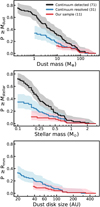 |
Fig. 1 Cumulative distribution of our sample in relation to the full Lupus disk population. Top panel: dust masses taken from Ansdell et al. 2016 of all Lupus disks detected in continuum (gray), Lupus disks resolved in continuum (blue) and our sample (red; see Sect. 2.2). Middle panel: same as above, but showing stellar masses derived from X-shooter spectra Alcalá et al. (2017), but recalculated using the new Gaia DR2 distances (see Appendix A in Alcalá et al. 2019). Bottom panel: same as above, but showing dust outer radii (Rmm). |
3.2 Chemical network
We use the CO isotopolog chemical network from Miotello et al. (2014) which includes both CO freeze-out and photodissociation of 12CO and its 13CO, C17O, and C18O isotopologs individually. This is an extension of the standard chemical network in DALI, which is based on the UMIST 06 network (Woodall et al. 2007; Bruderer et al. 2012; Bruderer 2013). Reactions included in the network are H2 formation on the grains, freeze-out, thermal and non-thermal desorption, hydrogenation of simple species on ices, gas-phase reactions, photodissociation, X-ray- and cosmic-ray-induced reactions, polycyclic aromatic hydrocarbon (PAH) grain charge exchange and/or hydrogenation, and reactions with vibrationallly excited H . The implementation of these reactions can be found in Appendix A.3.1 of Bruderer et al. (2012). Miotello et al. (2014) expanded the chemical network to include CO isotope-selective processes such as photodissociation (see also Visser et al. 2009).
3.3 The physical model
For the surface density of the model, we use the surface density profiles from Tazzari et al. (2017). These latter authors fitted the 890 μm visibilities of each source in our sample using a simple disk model with a tapered power law surface density and a two-layer temperaturestructure (see Chiang & Goldreich 1997). The tapered power law surface density is given by Lynden-Bell & Pringle (1974); Hartmann et al. (1998)
![\begin{equation*}\Sigma\,{=}\,\frac{\left(2-\gamma\right) M_{\textrm{disk}}}{2\pi R_{\textrm{c}}^2} \left(\frac{R}{R_{\textrm{c}}}\right)^{-\gamma} \exp\left[-\left(\frac{R}{R_{\textrm{c}}} \right)^{2-\gamma} \right], \end{equation*}](/articles/aa/full_html/2020/06/aa34537-18/aa34537-18-eq4.png) (1)
(1)
where Mdisk is the total disk mass, γ is the slope of the surface density, and Rc is the characteristic radius of the disk.
By using this surface density for the gas in our model, the gas and millimetre-sized grains follow the same surface density profile. Our null hypothesis is thus that no radial-dependent dust evolution has occurred.
3.3.1 Vertical structure
In their original fit, Tazzari et al. (2017) use a two-layer vertical structure to calculate the temperature structure of their models (see Chiang & Goldreich 1997). This vertical structure consists of a thin upper layer that intercepts and is superheated by the stellar radiation. This upper layer re-emits in the infrared and heats the interior of the disk. To correctly calculate the CO chemistry and emission, we instead need to run a full two-dimensional physical-chemical model. Assuming hydrostatic equilibrium and a vertically isothermal disk, the vertical density structure is given by a Gaussian distribution
![\begin{equation*}n(R,z)\,{=}\,\frac{1}{\sqrt{2 \pi}}\frac{1}{H} \exp \left[ -\frac{1}{2}\left(\frac{z}{H}\right)^2\right], \end{equation*}](/articles/aa/full_html/2020/06/aa34537-18/aa34537-18-eq5.png) (2)
(2)
where H = Rh is the physical height of the disk and the scale height h is parametrized by
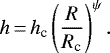 (3)
(3)
Here, hc is the scale height at Rc and ψ is known as the flaring angle. In this work, (hc, ψ) = (0.1, 0.1) is assumed for all disks.
Compared to the models fitted by Tazzari et al. (2017), our models have a different vertical structure and their temperature structure is calculateddifferently (cf. Sect. 3.1). It is therefore worthwhile to confirm that our models still reproduce the observed 890 μm continuum emission. As an example, Fig. 2 compares the model and observed 890 μm radial intensity profile for J16000236 - 4222115. As shown in the figure, our model matches the observation. Similar figures for all ten disksare shown in Fig. C.1. Except for Sz 133, our models reproduce the observed 890 μm radial intensity profile.
3.3.2 Total CO content
The gas outer radius is measured from 12CO emission and increases with the total CO content (see, e.g., Trapman et al. 2019). Observations revealed low 13CO and C18O line fluxes for most disks in Lupus, indicating that they have a low total CO content (see, e.g., Ansdell et al. 2016, 2018; Miotello et al. 2017).
Two explanations have been suggested to explain the low CO isotopolog line fluxes. CO isotopologs 13CO and C18O are often used to measure the total gasmass. The low 13CO and C18O line fluxes could indicate that these disks have low gas masses, suggesting low gas-to-dust mass ratios (Δgd) of the order of Δgd ≃ 1−10.
Alternatively, the low 13CO and C18O line fluxes could be due to an overall underabundance of volatile CO. In this case the disks do not have a low gas mass, but instead some process not currently accounted for has removed CO from the gas phase. Several processes have been suggested to explain the underabundance of CO. One possibility is linked to grain growth, where CO freezes out and becomes locked up in larger bodies, preventing it from re-entering the gas-phase chemistry (see, e.g., Bergin et al. 2010, 2016; Du et al. 2015; Kama et al. 2016). Alternatively, CO can be removed by converting it into more complex organics such as CH3OH that have higher freeze-out temperatures or turning it into CO2 and/or CH4 ice (see, e.g., Aikawa et al. 1997; Favre et al. 2013; Bergin et al. 2014; Bosman et al. 2018; Schwarz et al. 2018). We note that neither of these processes is included in DALI. Recent C2H observations in a subsample of Lupus disks are in agreement with this second hypothesis, that is, with C and O being underabundant in the gaseous outer disk (Miotello et al. 2019).
It should be noted here that the two explanations for the low total CO content discussed here have very different implications for the evolution of dust in the disk. If the low CO fluxes are indicative of low gas-to-dust mass ratios, dust grains will not be well coupled to the gas, increasing the effects of fragmentation and thus limiting the maximum grain size in the disk. If disks are underabundant in CO but have Δgd ~ 100, dust grains stay well coupled to the gas for longer and grow to larger sizes, and for most of the disks radial drift will set the maximum grain size.
For each source in our sample we examine both scenarios. We run a gas depleted disk model, where Δgd is lowered until the model reproduces the observed 13CO 3–2 line flux. In addition, we run a CO underabundant model for each source, where we lower the C and O abundances until the 13CO 3–2 line flux matches the observations. Our tests show that both approaches yield near identical results. In this work we therefore only show the CO underabundant models.
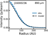 |
Fig. 2 Example comparison between model and observed 890 μm continuum intensity profile for J16000236-4222115. Similar comparisons for the other disks can be found in Fig. C.1. |
3.3.3 Dust properties
Dust settling is included parametrically in the model by splitting the grains into two populations:
-
Small grains (0.005–1 μm) are included with a (mass) fractional abundance 1−flarge and are assumed to be fully mixed with the gas.
-
Large grains (1–103 μm) are included with a fractional abundance flarge. To simulate the large grains settling to the midplane, these grains are constrained to a vertical region with scale height χh; χ < 1.
The opacities are computed using a standard interstellar medium (ISM) dust composition following Weingartner & Draine (2001), with a Mathis-Rumpl-Nordsieck (MNR, Mathis et al. 1977) grain size distribution between the grain sizes listed above.
In our models, we set flarge = 0.99 and χ = 0.2, thus assuming that the majority of the dust mass is in the large grains that have settled to the midplane of the disk.
We notethat in our analysis we keep the disk flaring structure and dust settling fixed and identical for all ten sources in our sample. In practice these parameters will likely vary between different disks. In Appendix B we show that varying these parameters changes RCO, mdl by less than 10%.
3.3.4 Stellar spectrum
Alcalá et al. (2014, 2017) used VLT X-shooter spectra to derive stellar properties for all our sources. Using their stellar luminosity and effective temperature, re-scaled to account for the new Gaia DR2 distances (see also Appendix A in Alcalá et al. 2019), we calculate the blackbody spectrum to use as the stellar spectrum for each source. Excess UV radiation that is expected as a result of accretion is added to the stellar spectrum as blackbody emission with T = 10 000 K. The total luminosity of this component is set to the observed accretion luminosity (Alcalá et al. 2017). For three sources (Sz 65, Sz 68 and MY Lup) only an upper limit of the accretion luminosity is known. We use this upper limit as the accretion luminosity in the models for these sources.
Some of the sources in our sample have anomalously low stellar luminosities, which could be linked to the high inclination of their disk. The main consequence of underestimating the stellar luminosity will be that our disk model is too cold. Increasing the stellar luminosity will have a very similar effect to increasing the flaring of the disk, as both increase the temperature in the disk. In Appendix B we show that increasing the flaring has only a minimal effect on the gas outer radius and therefore we do not expect an underestimation of the stellar luminosity to affect our results.
3.4 Measuring model outer radii
We follow the same approach as Ansdell et al. (2018) to measure the gas and dust outer radii from our models. These latter authors define the outer radius as that which encloses 90% of the total flux. In both the observations the gas outer radius (RCO) is measured from the 12CO 2–1 line emission and the dust outer radius (Rmm) is measured from the 1.3 millimeter continuum emission. The outer radius is measured using a curve of growth method where the flux is measured in increasingly larger elliptical apertures until the measured flux reaches 90% of the total flux. The inclination (i) and position angle (PA) of the apertures are chosen to match the orientation of the continuum emission (see Tazzari et al. 2017). A Keplerian masking technique is applied to the line emission to increase the S/N of the CO emission in the outer parts of the disk (for details, see Appendix A). Uncertainties on RCO and Rmm are determined by taking the uncertainties on the total flux and using the curve of growth method to propagate these uncertainties into the observed outer radius.
We measure RCO and Rmm from our models following the same procedure. First, our models are raytraced at the observed inclination and the resulting synthetic 12CO line emission cubes and 1.3 millimeter continuum emission maps are convolved with the beam of the Band 6 observations (see Sect. 2.1; Ansdell et al. 2018). We note that this approach is a simplification of producing full synthetic observationsof our models by sparsely sampling the Fourier transform of our model and reconstructing it in the image plane with the CLEAN algorithm. However, tests show that both methods yield approximately the same measured gas and dust outer radii.
For the CO, we add noise to the synthetic 12CO J = 2−1 spectral cube following the procedure outlined in Appendix D and we apply the Keplerian mask that was used for the observations before collapsing the spectral cube along the spectral axis to create a moment-zero map. The outer radii are measured using the curve of growth method, also using i and PA of the continuum for the elliptical apertures. Figure 3 shows a comparison between model and observed outer radii based on the 890 μm continuum emission. The models and observations agree to within 15% except for Sz 98 (~ 29%). Figures 2 and 3 show that our models are able to reproduce the continuum intensity profile and the extent of the 890 μm continuum observations.
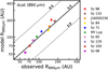 |
Fig. 3 Comparison between model and observed dust outer radii based on the 890 μm continuum emission. Differences are within 15% with the exception of Sz 98 (30%). |
4 Results
4.1 Observed versus modeled disk sizes
Having measured the gas and dust outer radii of our models, we can compare them to the observations. In Fig. 4 we compare the gas and dust outer radii of the model (RCO, mdl, Rmm, mdl) to the observed gas and dust outer radii (RCO, obs, Rmm, obs).
The top panel of Fig. 4 shows that all models are either equal in size to or smaller than the observations in terms of the measured gas outer radius. If we account for the uncertainty on RCO, obs shown in the figures as the colored error bar, we find that for six of the ten models (~ 60%) the modeled gas outer radius (RCO, mdl) is smaller than the observed gas outer radius (RCO, obs). These are predominantly the smaller disks (RCO, obs ≾ 200 AU).
The gray bars in Fig. 4 show the range of RCO, mdl that we measure after adding noise to the synthetic 12CO J = 2−1 spectral cube following the procedure outlined in detail in Appendix D. Briefly, we take a noise map from the observed spectral cube at random and add it to the model spectral cube, apply the Keplerian mask, and measure RCO, mdl using the curve of growth method outline in Sect. 3.4. This process is repeated for approximately 1000 noise realisation and gives us a distribution of possible RCO, mdl that could be measured from our models in the presence of noise (see Fig. D.1).
For most of our sources we see that the uncertainty on RCO, mdl, which is represented by the range of noisy RCO, mdl, is smaller than or similar to the uncertainty on RCO, obs. This shows that propagating the uncertainty in the total flux through the curve of growth into the observed outer radius is in most cases a conservative estimate of the effect of noise on measuring the outer radius.
The range of noisy RCO, mdl is the largest of the two smallest disks in the sample, Sz 68 and Sz 100 (see Fig. 4). Within our sample, these disks are also among the faintest in 12CO J = 2− 1 emission. The compact, faint emission makes their curve of growth more susceptible to the effects of noise. These results show that care should be taken when measuring the gas disk size of faint, compact disks using a curve of growth method.
The bottom panel of Fig. 4 compares modeled dust outer radius (Rmm, mdl) and observed dust outer radius (Rmm, obs), both measured from the 1.3 millimeter continuum emission. In the figure we can see that the Rmm, mdl of four disk models are significantly larger than Rmm, obs: namely Sz 84 (43%), Sz 71 (29%), J16000236 (23%), and Sz 98 (42%), and the disk model for MY Lup is significantly smaller (20%). The differences of Rmm between the model and the observations are larger than the differences seen at 890 μm (cf. Fig. 3). This indicates that our models overproduce the extent of the 1.3 millimeter continuum emission despite reproducing the extent of the continuum emission at 890 μm. A potential explanation for this is the lack of dust evolution in our models. Based on dust evolution, the larger 1.3 millimeter grains should be more concentrated toward the star compared to the 890 μm grains, which should be reflected by dust outer radii decreasing with wavelength (see, e.g., Tripathi et al. 2018). In our models we do not take this into account. Instead, we base our models on the 890 μm continuum emission, and thus the extent of the 890 μm grains, and assume the same radial extent for the 1.3 millimeter grains. The fact that Rmm, mdl is larger than Rmm, obs would therefore suggest that without including dust evolution we are overestimating the radial extent of the 1.3 millimeter grains.
4.2 Gas–dust size difference: models versus observations
The ratio between RCO and Rmm of a disk encodes whether it has undergone dust evolution. From the gas and dust outer radii of the models we can calculate their gas–dust size ratio (RCO, mdl∕Rmm, mdl). We note that, as the models do not include radial drift or radially dependent grain growth, these gas–dust size differences are set only by optical depth. Here we compare RCO, mdl∕Rmm, mdl to the observed gas–dust size difference (RCO, obs∕Rmm, obs), to identify which disks in our sample have undergone radial drift and radially dependent grain growth.
Our analysis of RCO∕Rmm is based on the fact that our models reproduce the extent of the continuum emission. However, in the previous section we found a seemingly systematic offset in Rmm, namely Rmm, mdl > Rmm, obs which might affect our interpretation of RCO, obs∕Rmm, obs versus RCO, mdl∕Rmm, mdl. We therefore elect to propagate the effect of this offset into RCO, mdl∕Rmm, mdl. We fit the offset with a straight line (Rmm, mdl = a × Rmm, obs + b, see Fig. 4) and use the best-fit values to scale Rmm, mdl when calculating RCO, mdl∕Rmm, mdl. We note that for the disks where Rmm, mdl > Rmm, obs this will increase RCO, mdl∕Rmm, mdl and enhance the perceived effect of optical depth on RCO∕Rmm. Therefore, for any disk showing RCO, obs∕Rmm, obs > RCO, mdl∕Rmm, mdl, we can confidently say that optical depth cannot explain their observed gas–dust size ratio.
Figure 5 shows RCO∕Rmm of the models and the observations. The gas–dust size ratios were calculated using the gas and dust outer radii shown in Fig. 4. The uncertainties on RCO, obs∕Rmm, obs were calculated using the uncertainties on RCO, obs and Rmm, obs. The uncertainties on RCO, mdl∕Rmm, mdl were calculated using the 16th and 84th quantile of the noisy RCO, mdl distribution (see Appendix E).
For five of the ten disks in our sample (50%) we find RCO, obs∕Rmm, obs > RCO, mdl∕Rmm, mdl even after the effects of noise are included, indicating this is a solid result considering the uncertainties on the measurements. These disks are Sz 65, Sz 71, J1600236, Sz 98, and Sz 129. For these disks, we need both dust evolution and optical depth effects to explain the observed RCO, obs∕Rmm, obs.
For the other five disks in the sample, Sz 133, Sz 100, MY Lup Sz 84, and Sz 68, the observed RCO, obs∕Rmm, obs lies within the uncertainty on RCO, mdl∕Rmm, mdl. For these disks, it is possible that our model would reproduce the observed RCO, obs∕Rmm, obs if it were observed at similar sensitivity to the band 6 observations. We are however not able rule out that the RCO, obs∕Rmm, obs measured for these five sources are only due to optical depth effects.
Among these latter five disks is Sz 68, also known as HT Lup, which has been observed at high spatial resolution as part of the DSHARP program (Andrews et al. 2018b, see also Kurtovic et al. 2018). Sz 68 is a multiple star system and the high-resolution observationswere able to individually detect both the primary disk around Sz 68 A and the disks around Sz 68 B and C located at 25 and 434 AU in projected separation from Sz 68 A (Kurtovic et al. 2018), respectively. In our observations with a resolution of ~ 39 AU the disks around Sz 68 A and B are not resolved separately. The observed RCO, obs∕Rmm, obs is therefore not likely to reflect the evolution of dust in this system.
It should be noted that of these five disks, three show large uncertainties towards large RCO, mdl∕Rmm, mdl, which can be traced back to similarly large uncertainties on RCO, mdl. Trapman et al. (2019) showed that a peak S∕N ≥ 10 on the moment-zero map of 12CO is required to measure RCO to within 20% (see, e.g., their Fig. H.1). To compare this to our observations, the peak S/N in our sample varies from ~ 6 (Sz 100) to ~ 12 (Sz 133). This suggests that for these three disks our comparison between RCO, obs∕Rmm, obs and RCO, mdl∕Rmm, mdl is probably not reliable due to observational effects. Observations with a factor two higher sensitivity, equivalent to increasing the integration time from 1 to 4 min per source, would be sufficient to remove these observational effects.
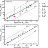 |
Fig. 4 Disk size comparison of the models and the observations. Top panel: gas disk size (RCO), defined as the radius enclosing 90% of the 12CO J = 2− 1 flux. Observed RCO, including uncertainties, are shown as a colored error bar (Ansdell et al. 2018). Gray vertical lines denote the range of RCO, mdl measured after noise is included (see Appendix D). The upper and lower points of the gray line show the 84th and 16th quantiles, respectively, of the noisy RCO distribution (cf. Appendix E). Bottom panel: as above, but showing the dust disk size, defined as the radius that encloses 90% of the 1.3 mm continuum flux. The blue dashed line shows the best fit of the offset between Rmm, mdl and Rmm, obs (see Sect. 4.2). |
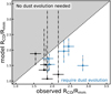 |
Fig. 5 Disk gas–dust size ratio comparison of the models with noise and the observations. Uncertainties of the model RCO, mdl∕Rmm, mdl were computed using the 16th and 84th quantile of the RCO distribution. Sources where RCO, mdl∕Rmm, mdl <RCO, obs∕Rmm, obs are shown in blue. To reproduce the observed RCO, obs∕Rmm, obs these sources require a combination of dust evolution and optical depth. |
5 Discussion
5.1 Fast dust evolution candidates in Lupus
In the present study, we look at the gas–dust size differences for a sample of 10 of the 48 disks in Lupus where 12CO J = 2−1 is detected. Our sample makes up ~15% of the Lupus disk population and is biased towards the most massive (≥ 10 M⊕) dust disks (see Fig. 1). Notably,the 12CO detections are not similarly biased, with 12CO J = 2−1 being detected for some of the faintest continuum sources.
Here we examine the 38 disks in Lupus where 12CO J = 2−1 was detected, but which did not meet our selection criteria; we refer to these as the “low-S/N sample”. As discussed in Sect. 2.2, most of these sources were excluded from our analysis because the S/N of the 12CO J = 2−1 was too low to measure RCO. Analyzing them in the same manner as the “high S/N sample” is not possible with the current observations. The disks in the high S/N sample show that RCO approximately coincides with a contour showing S∕N = 3 12CO J = 2−1 emission. For the disks in the low S/N sample we can therefore use the S∕N = 3 contour of 12CO J = 2−1 as a proxy for RCO, giving us some idea of their gas disk sizes. We note that this approximation is likely to underestimate RCO, as observing these sources at a sensitivity matching the high S/N sample would move the S∕N = 3 contour outward.
With this proxy for RCO, we can investigate whether the disks in the low S/N sample show signs of dust evolution. Using DALI, Trapman et al. (2019) compared the RCO, mdl∕Rmm, mdl of a series of models with and without dust evolution. These latter authors found that RCO∕Rmm ≥ 4 is a clear sign of dust evolution, giving us a clear criterion with which we can identify signs of dust evolution. If a disk in the low S/N sample has a S∕N = 3 contour for its 12CO emission that reaches beyond 4 × Rmm, it is likely that this disk would have RCO∕Rmm ≥ 4 if observed at higher sensitivity. We therefore identify it as a disk showing clear signs of having undergone dust evolution, where it would be difficult to explain the observations using only optical depth and without any radial drift or radially dependent grain growth.
As shown in Fig. 6 we identify six disks where the S∕N = 3 contour of their 12CO emission reaches beyond 4 × Rmm Of these, three have marginally resolved 1.3 mm continuum emission, namely J15450887 - 3417333, J16085324 - 3914401, and Sz 69. Although RCO could not be measured for these sources, it is difficult to explain the difference between the extent of the CO and the extent of the continuum without including dust evolution. It should be noted that the 12CO channel maps of J15450887 show some cloud emission. Most of this emission is removed by the Keplerian mask but some of it could still be present in the moment-zero map.
The other three disks remain unresolved in the continuum at a resolution of 0.′′ 25. As an upper limit for the dust disk size we use 0.′′125 which is approximately the radius of the beam. These three disks, Sz 130, V1192 Sco, and J16092697 - 3836269, show significant CO emission outside  0.′′125. Taking into account that the dust disk of these sources is unresolved, it is very likely that these disks have undergone substantial dust evolution. Noteworthy here is the inclusion of V1192 Sco, which has the faintest detected continuum flux of the disks in Lupus. Several studies have shown that there exists a relation between the millimeter luminosity and the dust disk size (see, e.g., Tazzari et al. 2017; Tripathi et al. 2017; Andrews et al. 2018b). If we extrapolate this relation down to the observed millimeter flux of V1192 Sco, we find a dust disk size of 4–8 AU (0.′′ 025–0.′′05). With 12CO J = 2−1 emission extending out up to 0.′′ 75, V1192 Sco would seemingly have a gas–dust size difference of RCO, obs∕Rmm, obs 15–30, which would make it one of the most extreme cases of grain growth and radial drift. Deeper observations of 12CO and higher resolution observations of the continuum are required to confirm this. We should note here that these disks could have faint, extended continuum emission that was undetected in our current observations. However, given the sensitivity of our current observations this faint emission can at most increase Rmm by a factor of two for our faintest source, V1192 Sco.
5.2 Are compact dust disks the result of runaway radial drift?
The discovery of six disks that likely have RCO, obs∕Rmm, obs ≥ 4 highlights an interesting property of the ten disks analyzed in detail in here, namely that they all have relatively low gas–dust size differences. The disks in our sample have ⟨ RCO, obs∕Rmm, obs ⟩obs = 2.06 ± 0.37 where the second number specifies the standard deviation of the sample. As discussed in Sect. 2.2, these disks represent the massive end of the Lupus disk population (see Fig. 1). In contrast, there are at least six disks with low dust masses that have RCO, obs∕Rmm, obs ≥ 4. These are all disks with compact continuum emission (Rmm ≤ 24 AU). We would expect more massive disks to have a higher RCO∕Rmm (see, e.g., Trapman et al. 2019). As a result of their higher disk mass, these disks have a greater total CO content which results in a larger observed gas outer radius (RCO). In addition, these disks have a higher dust mass, resulting in more efficient grain growth and inward radial drift.
The low RCO, obs∕Rmm, obs in our sample could be linked to the rings and gaps observed in large disks (see, e.g., Andrews et al. 2018a; Huang et al. 2018). These rings are the result of a local pressure maximum that acts as a dust trap for the millimeter-sized grains (see, e.g., Whipple 1972; Klahr & Henning 1997; Kretke & Lin 2007; Pinilla et al. 2012). These dust traps stop the millimeter-sized grains from drifting inward, effectively halting the radial dust evolution. As a result, the disks stay both large and bright in terms of the millimeter continuum emission. This hypothesis is also in line with recent results from a high-resolution ALMA survey in Taurus (Long et al. 2018, 2019). Of the 32 disks observed at ~ 16 AU resolution, all disks with a dust outer radius of at least 55 AU show detectable substructures (Long et al. 2019), whereas all disks without substructures are found to be small. Long et al. (2019) hypothesize that fast radial drift could be the cause of this dichotomy.
The disks in our sample are massive (Mdust = 10−200 M⊕) and should have been capable of forming gap-opening planets in the outer part of the disk. Using high-resolution observations of GW Lup (Sz 71), Zhang et al. (2018) inferred the presence of a ~ 10 M⊕ planet at 74 AU based on a gap in the continuum emission. The six disks of our sample with RCO, obs∕Rmm, obs ≥ 4 have a much lower dust mass (Mdust = 0.4−10 M⊕) and could have been unable to form a gap-opening planet in their outer disk. Without these gaps acting as dust traps, radial drift would be unimpeded, leading to a compact disk of millimeter-sized grains and a large gas–dust size difference.
Alternatively, the disks in our sample could have a higher level of CO underabundance, and therefore a lower total CO content, which would explain their low RCO, obs∕Rmm, obs (see, e.g., Sect. 3.3.2; Trapman et al. 2019). Being both large and massive, the disks in our sample are expected to be cold, leading to a larger fraction of CO being frozen out. A lower total CO content leads to a smaller RCO and a lower RCO∕Rmm.
Being compact and less massive, the six disks with RCO, obs∕Rmm, obs ≥ 4 are expected to be warmer. In these disks it would be harder to keep CO frozen out on the grains, lowering the effectiveness of the processes suggested to be responsible for the observed CO underabundance (see Sect. 3.3.2 and references therein). The lack of a CO underabundance would result in larger RCO and a higher RCO∕Rmm. However, Miotello et al. 2017 showed that Sz 90, J15450887 - 3417333, Sz 69, and Sz 130 have Δgd ≥ 10, indicating that they have a similar level of CO underabundance to the ten disks in our sample.
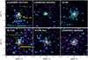 |
Fig. 6 12CO moment-zero maps of the six sources from the “low S/N sample” (see Sect. 5.1) where the S∕N = 3 contour of their 12CO emission, shown in cyan, reaches beyond 4 × Rmm. Using this contour as a proxy for RCO, these disks likely have RCO∕Rmm ≥ 4 and are therefore clear candidates for having undergone dust evolution (cf. Trapman et al. 2019). The top three disks have resolved continuum emission and their Rmm, obs is shown by the yellow ellipse. For these sources, Keplerian masking was applied to the 12CO J = 2− 1 emission (see Appendix A). The bottom three disks have unresolved continuum emission. The dashed yellow circle shows the size of the beam (0.′′ 25) as an upper limit to the dust disk size. Similarly, the dashed green circle shows four times the beam size. |
6 Conclusions
In the present study, the observed gas and dust size dichotomy in protoplanetary disks was studied in order to investigate the occurrence of common radial drift and radially dependent grain growth across the Lupus disk population. The gas structure of a sample of ten disks in the Lupus star-forming regions was modeled in detail using the thermochemical code DALI (Bruderer et al. 2012; Bruderer 2013), incorporating the effects of CO isotope-selective processes (Miotello et al. 2014). Surface density structures were based on modeling of the continuum emission by Tazzari et al. (2017). The total CO content of the models was fitted using integrated 13CO fluxes to account for either gas depletion or CO underabundance. Noise was added to the synthetic 12CO emission maps and gas and dust outer radii were measured from synthetic 12CO and 1.3 millimeter emission maps using the same steps used to measure these quantities from the observations. From comparisons of our model gas and dust outer radii to the observations, we draw the following conclusions:
-
For five disks (Sz 98, Sz 71, J16000236 - 4222115, Sz 129 and Sz 65) we find RCO, obs∕Rmm, obs > RCO, mdl∕Rmm, mdl. For these disks we need both dust evolution and optical depth effects to explain the observed gas–dust size difference.
-
For five disks (Sz 133, MY Lup, Sz 68, Sz 84 and Sz 100), the observed RCO, obs∕Rmm, obs lies within the uncertainties on RCO, mdl∕Rmm, mdl due to noise. For these disks the observed gas–dust size difference can be explained using optical line effects only.
-
We identify six disks without a measured RCO that show significant (S∕N ≥ 3) 12CO J = 2−1 emission beyond 4 × Rmm. These disks likely have RCO∕Rmm ≫ 4, which would be difficult to explain without substantial dust evolution.
-
The wide range of noisy RCO, mdl measured for the two smallest disks in our sample show that care should be taken when measuring the gas disks size of faint compact disks using a curve of growth method.
Our analysis shows that most of the disks in our sample, which represent the bright end of the Lupus disk population, are consistent with radial drift and grain growth. Furthermore, we also find six faint disks with 12CO emission beyond four times their dust disk size, suggesting that radial drift is a common feature among bright and faint disks. For both cases, our analysis is limited by the sensitivity of current disk surveys. More sensitive disk surveys that integrate 5–10 min per source are required to obtain a complete picture of radial drift and grain growth in “typical disks” in young star-forming regions.
Acknowledgements
We would like to thank the referee for constructive and detailed comments that greatly improved the presentationof the paper. We would also like to thank A. Bosman, L. Testi and M. Tazzari for the useful discussions. LT and MRH are supported by NWO grant 614.001.352. M.A. acknowledges support from NSF AST-1518332, NASA NNX15AC89G and NNX15AD95G/NEXSS. This work benefited from NASA’s Nexus for Exoplanet System Science (NExSS) research coordination network sponsored by NASA’s Science Mission Directorate. Astrochemistry in Leiden is supported by the European Union A-ERC grant 291141 CHEMPLAN, by the Netherlands Research School for Astronomy (NOVA), and by a Royal Netherlands Academy of Arts and Sciences (KNAW) professor prize. SF and CFM are supported by ESO fellowships. JPW is supported NASA grant NNX15AC92G. This paper makes use of the following ALMA data: 2013.1.00220.S, 2015.1.00222.S, 2013.1.00226.S, 2013.00694. ALMA is a partnership of ESO (representing its member states), NSF (USA) and NINS (Japan), together with NRC (Canada), NSC and ASIAA (Taiwan), and KASI (Republic ofKorea), in cooperation with the Republic of Chile. The Joint ALMA Observatory is operated by ESO, AUI/NRAOand NAOJ. All figures were generated with the PYTHON-based package MATPLOTLIB (Hunter 2007).
Appendix A Keplerian masking
Analysis of the gas emission of protoplanetary disks is often performed using the moment-zero map, which is obtained by integrating the observed spectral cube along the velocity axis. The velocity range for the integration is set by the maximum velocity offset (positive and negative) relative to the source velocity where emission of the disk is still observed. This leads to broad velocity integration range, whereas in the outer regions of the disk line emission is coming from a much more narrower velocity range. The S/N in these regions can therefore be improved if the integration is limited to only those channels containing emission.
This method of improving the S/N of moment-zero maps has already been used (e.g., Salinas et al. 2016; Carney et al. 2017; Bergner et al. 2018; Loomis et al. 2018). Yen et al. (2016) developed a similar method whereby spectra are aligned at different positions in the disk by shifting them by the projected Keplerian velocities at their positions and are then stacked. Their method produces an aligned spectrum with increased S/N, well suited for detecting emission not seen in individual channels (e.g., Yen et al. 2018).
The masking method works for observed line emission from a source with a known, ordered velocity pattern. In the case of protoplanetary disks, this is the Keplerian rotation around the central star. Using prior knowledge of this rotation pattern, voxels of the spectral cube can be selectively included in the analysis of the data, for example when making a moment-zero map, based on the criterion
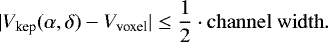 (A.1)
(A.1)
Here, Vkep is the Keplerian velocity at the coordinates (RA, Dec) = (α, δ) and Vvoxel is the velocity coordinate of the voxel.
A.1 Implementation
A.1.1 Calculate the projected Keplerian velocity pattern
In order to calculate the Keplerian velocities at a given point p with coordinates (α, δ) in the observed image, the coordinates of p first have to be projected onto the 2D local frame of the source. For a source with an observed position angle PA and inclination i at a distance d this coordinate transformation is given by
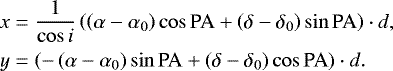
Here α, δ are the right ascension and declination of the point p and (α0, δ0) is the location of the center of the source.
Using the local coordinates x, y the Keplerian velocity at p can be calculated using
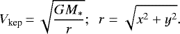 (A.4)
(A.4)
Here G is the gravitational constant, M* is the stellar mass, and r is the deprojected radial distance from the star.
To convert the Keplerian velocity back to the velocity at which the emission will be observed, it has to be projected along the line of sight:
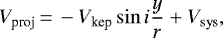 (A.5)
(A.5)
where Vsys is the systematic velocity of the source.
A.1.2 Selecting voxels containing emission
For a given point p = (α, δ) Eq. (A.5) gives the expected velocity of the emission. Based on this information a Keplerian mask can be created by selecting a voxel nml for the Keplerian mask if
 (A.6)
(A.6)
Here αn, δm, Vl are the coordinates of the voxel and ΔVwidth is the channel width. Further, ΔVint is introduced in Eq. (A.6) to compensate for the fact that using a Keplerian rotation profile is a simplification that is only valid if the disk is geometrically thin and the rotation is purely Keplerian. In reality, the line emission is more likely to originate from layers higher in the (often flared) disk (e.g., Dutrey et al. 2014). As a result a single pixel, representing a single line of sight through the disk, contains contributions from different vertical layers at project velocities that are offset from the Keplerian rotation velocity of the midplane.
Here ΔVint is left as a free parameter with no radial dependence in order to make no assumptions on the vertical structure of the disk. However, such a dependence could be introduced. For example Yen et al. (2016) use the empirically fitted description for ΔVint from Piétu et al. (2007).
A.1.3 Convolving the mask
After the mask is set up, it is convolved with the beam to include the effects of resolution on the channel maps. We note that this effect is only relevant if the smearing by the beam is much larger than the width of the channel.
A.1.4 Clipping the mask
In order to ensure flux conservation in the masked region, a final step has to be made. After the convolution in the previous step, the pixels of the mask now have weights ≤1. The mask is therefore converted back into a boxcar function according to
 (A.7)
(A.7)
where M is the mask after step 3 and the cutoff is set to 0.05 of the peak value.
A.2 Making moment-zero maps and calculating noise
After the mask has been produced following the steps mentioned above, it can be applied to the data. The moment-zero map can be calculated following
 (A.8)
(A.8)
where I(αn, δm, Vl) is the observed spectral cube and V0 and VL are the minimum and maximum velocities of the spectral cube respectively.
In a similar manner, a map of the expected noise levels in the moment-zero map can be calculated. As a result of the masking, individual pixels will have different noise characteristics depending on how many nonzero voxels in the mask are summed over (cf. Eq. (A.8)). Using the fact that the noise between individual channels is independent, a 2D noise map can be created using
 (A.9)
(A.9)
where RMS is the root mean square noise taken from an empty channel.
Keplerian masks.
As a result of the term in the square root, the S/N defined as S∕N ≡Mom 0∕N can be increasedby not clipping the mask (Sect. A.1.4), but this comes at the cost of a reduced total flux in the moment-zero map. This difference can be understood by the fact that the convolved mask provides lower weights (wnml) for voxels that are expected to contain very little flux with respect to the noise in that pixel. In the noise, these voxels are almost excluded due to the term  in Eq (A.9), resulting in a lower noise for that pixel. In the moment-zero map however, the flux in these voxels is also scaled down by a factor wnml. As wnml ≤ 1, flux is no longer conserved in this case.
A.3 Caveats
In step one of making the mask (Sect. A.1.1), a simplification is made in that a single velocity can be assigned to a pixel, i.e., that the velocity gradient over the length of pixel is small. At the center this simplification breaks down. To circumvent this problem the center pixel can be included in all channels.
We note that as a consequence the S/N in the center part decreases to the pre-masked values. For most sources this is not a significant problem, as the S/N is usually highest at the center where the source is brightest.
A.4 The Keplerian mask parameters of our sample
Here we outline the Keplerian mask used in this work. As shown in Eq. (A.6) the Keplerian mask is described by seven parameters: the stellar mass (M*), the orientation of the disk (PA, i), the three coordinate centroids (α0, δ0, Vsys), and the free parameter ΔVint. For the stellar masses we use the observations and methods presented in Alcalá et al. (2014, 2017), but rescaled to the new Gaia DR2 distances (Brown et al. 2018, see also Appendix A of Manara et al. 2018). The position angle, inclination, and centroid were taken from the observations of the millimeter continuum (cf. Tables 1 and 2 in Tazzari et al. 2017). The final two parameters, Vsys and ΔVint, were obtained by varying them to maximize the total S/N in the moment-zero map. The mask parameters of the ten sources in our sample plus the eight sources with resolved continuum emission described in Sect. 5.1 are presented in Table A.1.
Appendix B Influence of dust settling and flaring
In our models we have kept the disk vertical structure fixed. In addition we assume a single height and mass fraction of large grains (cf. Sects. 3.3.1 and 3.3.3). The vertical structure and the distribution of the large grains set both the temperature structure and the chemistry. Varying them could therefore change the 13CO 3–2 flux used to determine the total CO content and the shape of 12CO intensity profile from which we measure RCO. We examinethe effect of varying the vertical structure and the distribution of the large grains on RCO for two disks in our sample that represent two completely different physical structures: Sz 68 (compact, strong CO flux, 13CO optically thick) and Sz 98 (large, weak CO flux, 13CO optically thin).
The results are shown in Fig. B.1. The top three panels show the effect on the 13CO integrated flux used to determine the total CO content of the disk (cf. Sect. 3.3.2). Increasing the vertical extent of the large grains (χ) lowers the 13CO flux by up to ~ 40% for the optically thin Sz 98 and up to ~80% for the optically thick Sz 68. This is likely due to the dust becoming optically thick at millimeter wavelengths higher up in the disk. Decreasing the mass fraction of large grains (flarge) also lowers the 13CO flux, up to ~ 25% for both disks. Changing either χ or flarge would require increasing the total CO content to reproduce the 13CO flux, which would increase RCO.
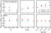 |
Fig. B.1 Effects of vertical structure and the large grains. Top panels: integrated 13CO flux as function of large grain settling (χ), fraction of large grains (flarge) and disk vertical structure ( |
Changing the vertical structure of the disk by either increasing the amount of flaring or increasing the scale height of the disk will lead by to an increase in the observed 13CO integrated flux. Both parameters directly affect the amount of stellar light intercepted by the disk, leading to a higher temperature. The 13CO flux is increased by up to ~20% for Sz 68 and up to ~65% for Sz 98. Increasing either the flaring or the scale height would mean a lower total CO content is needed to match the observed 13CO flux, leading to a smaller RCO (cf. Trapman et al. 2019).
The bottom three panels of Fig. B.1 show how RCO is affected by changes in flarge, χ, hc, Ψ. For Sz 98 the gas outer radius increases by less than 10% if either flarge or χ is changed and the RCO of Sz 68 is not affected at all. Changing the vertical structure of either disk changes the derived Rgas by less than 5%. The vertical structure does affect the 12CO intensity profile, but the relative changes remain nearly constant over the extent of the disk. As a result the curve of growth and the inferred Rgas remain unaffected.
Appendix C Radial 890 μm continuum profiles
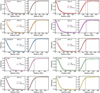 |
Fig. C.1 Comparison between model and observed 890 μm continuum intensity profiles for the ten sources in our sample. For each source, the left panel shows the intensity profile and the right panel shows the matching normalized curve of growth for both the model (black, dashed) and the observation (colored, solid). Vertical lines in the right panels show the radius that encloses 90% of the total flux (R890 μm). We note that the curve of growth of the model and the observation are normalized separately as the total flux is unimportantwhen measuring R890 μm. |
Appendix D Measuring RCO from noisy spectral cube
Here, we outline how noise was added to models to simulate its effect on measuring RCO from our models. Theprocedure can be outlined in three steps. First a random patch of noise is added to each of the channels in the synthetic 12CO spectral cube. The patch of noise is taken from one of the emission free channels in observed spectral cube. Care is taken to avoid the outer edges of the observed field of view in the random selection, as the noise levels there are not representative for the center of the observations.
Next, we construct a Keplerian mask using the same parameters that are used for the observations (cf. Table A.1). By applyingthe Keplerian mask to the noisy model spectral cube we increase the S/N in the outer parts of the disk in the same manner as in the observations (cf. Sect. 3.4). The masked spectral cube is summed over the velocity axis to create the 12CO moment-zero map.
Finally, the gas outer radius is measured from the noisy moment-zero map. By definition, RCO is the radius that encloses 90% of the total flux (Ftot). In noiseless case, the curve of growth converges to Ftot at large radii. In the presence of noise the curve of growth can show variations at large radii, making it difficult to determine Ftot (cf. Fig. D.1). Empirically, we find that using the flux at the first peak in the curve of growth in most cases most closely matches Ftot of the noiseless case. At an average peak S∕N ~ 8 of the 12CO moment-zero map, noise has a significant effect on measuring RCO. As an example, Fig. D.1 shows the curve of growths for four noise realizations for the Sz 129 disk model. As shown in the figure, the curve of growth varies between each noise realization and all four have different Ftot and different RCO.
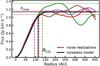 |
Fig. D.1 Curve of growth of the 12CO 2–1 emission for the Sz 129 model for four different and extreme noise realizations chosen to show the range of effects that noise can have on measuring the outer radius. For each noise realization, the horizontal lines show the total flux and the dashed vertical line shows the calculated outer radius. The curve of growth, total flux, and outer radius of the noiseless model are shown in black. |
Appendix E Noisy RCO distributions for the disks in our sample
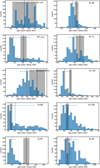 |
Fig. E.1 Histogram of possible RCO if noise is included in the model. The 16th quantile and the 84th quantile are shown by the blue errorbar, with the median shown as a blue vertical line. Orange vertical line shows RCO of the noiseless model. The observed RCO and uncertainties are shown in black. |
Appendix F 12CO J = 2−1 emission maps of 17 sources
In total, 48 disks in Lupus were detected in 12CO J = 2−1. In this work we analyzed ten of these disks in detail (referred to as the high S/N sample) and showed 12CO J = 2−1 emission maps of six more disks (part of the low S/N sample; see Sect. 5.1). Here we show the 12CO J = 2−1 emission maps of the remaining disks of the low S/N sample. From our analysis we exclude transition disks with clear resolved cavities. Fora detail analysis of these disks, see van der Marel et al. (2018).
The remaining 17 disks with detected 12CO emission can be divided into two groups. For 6 of the 17 disks the 1.3 millimeter continuum emission was resolved and we were able to measure Rmm (see also Tazzari et al. 2017). The top two rows of Fig. F.1 show the 12CO 2–1 moment-zero maps for these six sources. Keplerian masking was applied to the data before making the moment-zero maps (cf. Sect. 3.4 and Appendix A).
Sz 83, also known as RU Lup, is a notable inclusion here. This disk is the third-most brightest continuum source in Lupus and has been readily detected in 12CO, 13CO, and C18O. Furthermore, RU Lup hasalso been observed at high spatial resolution as part of the DSHARP program (Andrews et al. 2018a). It seems therefore odd that RCO has not been measured for this source. A closer inspection of the 12CO channel maps reveals that a component of the emission is non Keplerian and could be a possible outflow (see Appendix C in Ansdell et al. 2018). Keplerian masking has removed part of the emission but enough remains in the moment-zero map to prevent us from measuring RCO.
There are 11 disks that are detected in 12CO but for which the 1.3 millimeter continuum emission is not resolved at a resolution of 0.′′ 25. These are shown in the bottom four rows of Fig. F.1. We exclude three disks from our analysis: J16011549 - 4152351 is resolved in the continuum, but the 12CO channel maps show significant cloud emission even after applying Keplerian masking. J16070384 - 3911113 and J16090141 - 3925119 are resolved but have irregular shaped continuum emission and are possibly unresolved binary sources (cf. Tazzari et al. 2017).
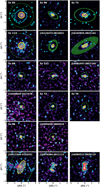 |
Fig. F.1 12CO moment-zero maps of the 17 sources that were detected at low S/N, referred to as the low S/N sample in this work. Cyan contours show significant (S∕N ≥ 3) 12CO emission. The top six disks have resolved continuum emission and their Rmm, obs is shown by the yellow ellipse. For these sources, Keplerian masking was applied to the 12CO J = 2− 1 emission (see Appendix A). The middle eight disks (Sz 66 to J16095628) have unresolved continuum emission. The dashed yellow circle shows the size of the beam (0.′′ 25) as an upper limit to the dust disk size. Similarly, the dashed green circle shows four times the beamsize. For J16011549 the continuum is resolved and Rdust was calculated from 90% of the total flux. The continuum emission of J16070384 and J16090141 is resolved but irregular in shape. Here, we show the 3σ contours of the continuum in green. |
References
- Aikawa, Y., Umebayashi, T., Nakano, T., & Miyama, S. M. 1997, ApJ, 486, L51 [NASA ADS] [CrossRef] [Google Scholar]
- Alcalá, J., Natta, A., Manara, C., et al. 2014, A&A, 561, A2 [NASA ADS] [CrossRef] [EDP Sciences] [Google Scholar]
- Alcalá, J., Manara, C., Natta, A., et al. 2017, A&A, 600, A20 [NASA ADS] [CrossRef] [EDP Sciences] [Google Scholar]
- Alcalá, J. M., Manara, C. F., France, K., et al. 2019, A&A, 629, A108 [NASA ADS] [CrossRef] [EDP Sciences] [Google Scholar]
- Andrews, S. M., Wilner, D. J., Hughes, A., et al. 2011, ApJ, 744, 162 [Google Scholar]
- Andrews, S. M., Rosenfeld, K. A., Kraus, A. L., & Wilner, D. J. 2013, ApJ, 771, 129 [NASA ADS] [CrossRef] [Google Scholar]
- Andrews, S. M., Huang, J., Pérez, L. M., et al. 2018a, ApJ, 869, L41 [NASA ADS] [CrossRef] [Google Scholar]
- Andrews, S. M., Terrell, M., Tripathi, A., et al. 2018b, ApJ, 865, 157 [NASA ADS] [CrossRef] [Google Scholar]
- Ansdell, M., Williams, J. P., van der Marel, N., et al. 2016, ApJ, 828, 46 [Google Scholar]
- Ansdell, M., Williams, J. P., Manara, C. F., et al. 2017, AJ, 153, 240 [NASA ADS] [CrossRef] [EDP Sciences] [Google Scholar]
- Ansdell, M., Williams, J. P., Trapman, L., et al. 2018, ApJ, 859, 21 [NASA ADS] [CrossRef] [Google Scholar]
- Bailer-Jones, C. A. L., Rybizki, J., Fouesneau, M., Mantelet, G., & Andrae, R. 2018, AJ, 156, 58 [NASA ADS] [CrossRef] [Google Scholar]
- Barenfeld, S. A., Carpenter, J. M., Ricci, L., & Isella, A. 2016, ApJ, 827, 142 [NASA ADS] [CrossRef] [Google Scholar]
- Barenfeld, S. A., Carpenter, J. M., Sargent, A. I., Isella, A., & Ricci, L. 2017, ApJ, 851, 85 [NASA ADS] [CrossRef] [Google Scholar]
- Benz, W., Ida, S., Alibert, Y., Lin, D., & Mordasini, C. 2014, in Protostars and Planets VI, eds. H. Beuther, R. S. Klessen, C. P. Dullemond, & T. Henning, 691 [Google Scholar]
- Bergin, E., Hogerheijde, M., Brinch, C., et al. 2010, A&A, 521, L33 [NASA ADS] [CrossRef] [EDP Sciences] [Google Scholar]
- Bergin, E., Cleeves, L. I., Crockett, N., & Blake, G. 2014, Faraday Discussions, 168, 61 [NASA ADS] [CrossRef] [Google Scholar]
- Bergin, E. A., Du, F., Cleeves, L. I., et al. 2016, ApJ, 831, 101 [NASA ADS] [CrossRef] [Google Scholar]
- Bergner, J. B., Guzmán, V. G., Öberg, K. I., Loomis, R. A., & Pegues, J. 2018, ApJ, 857, 69 [NASA ADS] [CrossRef] [Google Scholar]
- Birnstiel, T., & Andrews, S. M. 2013, ApJ, 780, 153 [Google Scholar]
- Birnstiel, T., Ricci, L., Trotta, F., et al. 2010, A&A, 516, L14 [NASA ADS] [CrossRef] [EDP Sciences] [Google Scholar]
- Birnstiel, T., Klahr, H., & Ercolano, B. 2012, A&A, 539, A148 [NASA ADS] [CrossRef] [EDP Sciences] [Google Scholar]
- Bosman, A. D., Walsh, C., & van Dishoeck, E. F. 2018, A&A, 618, A182 [NASA ADS] [CrossRef] [EDP Sciences] [Google Scholar]
- Brown, A., Vallenari, A., Prusti, T., et al. 2018, A&A, 616, A1 [NASA ADS] [CrossRef] [EDP Sciences] [Google Scholar]
- Bruderer, S. 2013, A&A, 559, A46 [NASA ADS] [CrossRef] [EDP Sciences] [Google Scholar]
- Bruderer, S., van Dishoeck, E. F., Doty, S. D., & Herczeg, G. J. 2012, A&A, 541, A91 [NASA ADS] [CrossRef] [EDP Sciences] [Google Scholar]
- Carney, M. T., Hogerheijde, M. R., Loomis, R. A., et al. 2017, A&A, 605, A21 [NASA ADS] [CrossRef] [EDP Sciences] [Google Scholar]
- Cazzoletti, P., Manara, C. F., Baobab Liu, H., et al. 2019, A&A, 626, A11 [NASA ADS] [CrossRef] [EDP Sciences] [Google Scholar]
- Chiang, E. I., & Goldreich, P. 1997, ApJ, 490, 368 [NASA ADS] [CrossRef] [Google Scholar]
- Cieza, L. A., Ruíz-Rodríguez, D., Hales, A., et al. 2019, MNRAS, 482, 698 [NASA ADS] [CrossRef] [Google Scholar]
- Cox, E. G., Harris, R. J., Looney, L. W., et al. 2017, ApJ, 851, 83 [Google Scholar]
- Du, F., Bergin, E. A., & Hogerheijde, M. R. 2015, ApJ, 807, L32 [NASA ADS] [CrossRef] [Google Scholar]
- Dutrey, A., Guilloteau, S., Prato, L., et al. 1998, A&A, 338, L63 [NASA ADS] [Google Scholar]
- Dutrey, A., Semenov, D., Chapillon, E., et al. 2014, Protostars and Planets VI (Tucson: University of Arizona Press), 317 [Google Scholar]
- Facchini, S., Birnstiel, T., Bruderer, S., & van Dishoeck, E. F. 2017, A&A, 605, A16 [NASA ADS] [CrossRef] [EDP Sciences] [Google Scholar]
- Facchini, S., van Dishoeck, E. F., Manara, C. F., et al. 2019, A&A, 626, L2 [NASA ADS] [CrossRef] [EDP Sciences] [Google Scholar]
- Favre, C., Cleeves, L. I., Bergin, E. A., Qi, C., & Blake, G. A. 2013, ApJ, 776, L38 [NASA ADS] [CrossRef] [Google Scholar]
- Frasca, A., Biazzo, K., Alcalá, J. M., et al. 2017, A&A, 602, A33 [NASA ADS] [CrossRef] [EDP Sciences] [Google Scholar]
- Guilloteau, S.,& Dutrey, A. 1998, A&A, 339, 467 [NASA ADS] [Google Scholar]
- Guilloteau, S., Dutrey, A., Piétu, V., & Boehler, Y. 2011, A&A, 529, A105 [NASA ADS] [CrossRef] [EDP Sciences] [Google Scholar]
- Hartmann, L., Calvet, N., Gullbring, E., & D’Alessio, P. 1998, ApJ, 495, 385 [NASA ADS] [CrossRef] [Google Scholar]
- Huang, J., Andrews, S. M., Dullemond, C. P., et al. 2018, ApJ, 869, L42 [NASA ADS] [CrossRef] [Google Scholar]
- Hughes, A., Wilner, D., Qi, C., & Hogerheijde, M. 2008, ApJ, 678, 1119 [NASA ADS] [CrossRef] [Google Scholar]
- Hunter, J. D. 2007, Comput. Sci. Eng., 9, 90 [NASA ADS] [CrossRef] [Google Scholar]
- Kama, M., Bruderer, S., van Dishoeck, E. F., et al. 2016, A&A, 592, A83 [NASA ADS] [CrossRef] [EDP Sciences] [Google Scholar]
- Klahr, H. H., & Henning, T. 1997, Icarus, 128, 213 [NASA ADS] [CrossRef] [Google Scholar]
- Kretke, K. A., & Lin, D. N. C. 2007, ApJ, 664, L55 [NASA ADS] [CrossRef] [Google Scholar]
- Kurtovic, N. T., Pérez, L. M., Benisty, M., et al. 2018, ApJ, 869, L44 [NASA ADS] [CrossRef] [Google Scholar]
- Long, F., Herczeg, G. J., Pascucci, I., et al. 2017, ApJ, 844, 99 [NASA ADS] [CrossRef] [Google Scholar]
- Long, F., Pinilla, P., Herczeg, G. J., et al. 2018, ApJ, 869, 17 [NASA ADS] [CrossRef] [Google Scholar]
- Long, F., Herczeg, G. J., Harsono, D., et al. 2019, ApJ, 882, 49 [NASA ADS] [CrossRef] [Google Scholar]
- Loomis, R. A., Cleeves, L. I., Öberg, K. I., et al. 2018, ApJ, 859, 131 [NASA ADS] [CrossRef] [Google Scholar]
- Lynden-Bell, D., & Pringle, J. E. 1974, MNRAS, 168, 603 [NASA ADS] [CrossRef] [Google Scholar]
- Manara, C. F., Morbidelli, A., & Guillot, T. 2018, A&A, 618, L3 [NASA ADS] [CrossRef] [EDP Sciences] [Google Scholar]
- Mathis, J. S., Rumpl, W., & Nordsieck, K. H. 1977, ApJ, 217, 425 [NASA ADS] [CrossRef] [Google Scholar]
- Menu, J., Van Boekel, R., Henning, T., et al. 2014, A&A, 564, A93 [NASA ADS] [CrossRef] [EDP Sciences] [Google Scholar]
- Merín, B., Jørgensen, J., Spezzi, L., et al. 2008, ApJS, 177, 551 [NASA ADS] [CrossRef] [Google Scholar]
- Miotello, A., Robberto, M., Potenza, M. A. C., & Ricci, L. 2012, ApJ, 757, 78 [NASA ADS] [CrossRef] [Google Scholar]
- Miotello, A., Bruderer, S., & van Dishoeck, E. F. 2014, A&A, 572, A96 [NASA ADS] [CrossRef] [EDP Sciences] [Google Scholar]
- Miotello, A., van Dishoeck, E., Williams, J., et al. 2017, A&A, 599, A113 [NASA ADS] [CrossRef] [EDP Sciences] [Google Scholar]
- Miotello, A., Facchini, S., van Dishoeck, E. F., et al. 2019, A&A, 631, A69 [NASA ADS] [CrossRef] [EDP Sciences] [Google Scholar]
- Morton, T. D., Bryson, S. T., Coughlin, J. L., et al. 2016, ApJ, 822, 86 [NASA ADS] [CrossRef] [Google Scholar]
- Panić, O., Hogerheijde, M. R., Wilner, D., & Qi, C. 2008, A&A, 491, 219 [NASA ADS] [CrossRef] [EDP Sciences] [Google Scholar]
- Pascucci, I., Testi, L., Herczeg, G., et al. 2016, ApJ, 831, 125 [NASA ADS] [CrossRef] [Google Scholar]
- Pérez, L. M., Carpenter, J. M., Chandler, C. J., et al. 2012, ApJ, 760, L17 [NASA ADS] [CrossRef] [Google Scholar]
- Pérez, L. M., Chandler, C. J., Isella, A., et al. 2015, ApJ, 813, 41 [NASA ADS] [CrossRef] [Google Scholar]
- Piétu, V., Dutrey, A., & Guilloteau, S. 2007, A&A, 467, 163 [NASA ADS] [CrossRef] [EDP Sciences] [Google Scholar]
- Pinilla, P., Birnstiel, T., Ricci, L., et al. 2012, A&A, 538, A114 [NASA ADS] [CrossRef] [EDP Sciences] [Google Scholar]
- Salinas, V. N., Hogerheijde, M. R., Bergin, E. A., et al. 2016, A&A, 591, A122 [NASA ADS] [CrossRef] [EDP Sciences] [Google Scholar]
- Schwarz, K. R., Bergin, E. A., Cleeves, L. I., et al. 2018, ApJ, 856, 85 [NASA ADS] [CrossRef] [Google Scholar]
- Tazzari, M., Testi, L., Ercolano, B., et al. 2016, A&A, 588, A53 [NASA ADS] [CrossRef] [EDP Sciences] [Google Scholar]
- Tazzari, M., Testi, L., Natta, A., et al. 2017, A&A, 606, A88 [NASA ADS] [CrossRef] [EDP Sciences] [Google Scholar]
- Trapman, L., Facchini, S., Hogerheijde, M. R., van Dishoeck, E. F., & Bruderer, S. 2019, A&A, 629, A79 [NASA ADS] [CrossRef] [EDP Sciences] [Google Scholar]
- Tripathi, A., Andrews, S. M., Birnstiel, T., & Wilner, D. J. 2017, ApJ, 845, 44 [NASA ADS] [CrossRef] [Google Scholar]
- Tripathi, A., Andrews, S. M., Birnstiel, T., et al. 2018, ApJ, 861, 64 [NASA ADS] [CrossRef] [Google Scholar]
- van der Marel,N., Williams, J. P., Ansdell, M., et al. 2018, ApJ, 854, 177 [NASA ADS] [CrossRef] [Google Scholar]
- Visser, R., van Dishoeck, E. F., & Black, J. H. 2009, A&A, 503, 323 [NASA ADS] [CrossRef] [EDP Sciences] [Google Scholar]
- Ward-Duong, K., Patience, J., Bulger, J., et al. 2018, AJ, 155, 54 [NASA ADS] [CrossRef] [Google Scholar]
- Weingartner, J. C., & Draine, B. 2001, ApJ, 548, 296 [NASA ADS] [CrossRef] [Google Scholar]
- Whipple, F. L. 1972, in From Plasma to Planet, ed. A. Elvius (Hoboken: Wiley), 211 [Google Scholar]
- Williams, J. P., Cieza, L., Hales, A., et al. 2019, ApJ, 875, L9 [Google Scholar]
- Woodall, J., Agúndez, M., Markwick-Kemper, A., & Millar, T. 2007, A&A, 466, 1197 [NASA ADS] [CrossRef] [EDP Sciences] [Google Scholar]
- Yen, H.-W., Liu, H. B., Gu, P.-G., et al. 2016, ApJ, 820, L25 [NASA ADS] [CrossRef] [Google Scholar]
- Yen, H.-W., Koch, P. M., Manara, C. F., Miotello, A., & Testi, L. 2018, A&A, 616, A100 [NASA ADS] [CrossRef] [EDP Sciences] [Google Scholar]
- Zhang, S., Zhu, Z., Huang, J., et al. 2018, ApJ, 869, L47 [NASA ADS] [CrossRef] [Google Scholar]
All Tables
All Figures
|
Fig. 1 Cumulative distribution of our sample in relation to the full Lupus disk population. Top panel: dust masses taken from Ansdell et al. 2016 of all Lupus disks detected in continuum (gray), Lupus disks resolved in continuum (blue) and our sample (red; see Sect. 2.2). Middle panel: same as above, but showing stellar masses derived from X-shooter spectra Alcalá et al. (2017), but recalculated using the new Gaia DR2 distances (see Appendix A in Alcalá et al. 2019). Bottom panel: same as above, but showing dust outer radii (Rmm). |
| In the text | |
|
Fig. 2 Example comparison between model and observed 890 μm continuum intensity profile for J16000236-4222115. Similar comparisons for the other disks can be found in Fig. C.1. |
| In the text | |
|
Fig. 3 Comparison between model and observed dust outer radii based on the 890 μm continuum emission. Differences are within 15% with the exception of Sz 98 (30%). |
| In the text | |
|
Fig. 4 Disk size comparison of the models and the observations. Top panel: gas disk size (RCO), defined as the radius enclosing 90% of the 12CO J = 2− 1 flux. Observed RCO, including uncertainties, are shown as a colored error bar (Ansdell et al. 2018). Gray vertical lines denote the range of RCO, mdl measured after noise is included (see Appendix D). The upper and lower points of the gray line show the 84th and 16th quantiles, respectively, of the noisy RCO distribution (cf. Appendix E). Bottom panel: as above, but showing the dust disk size, defined as the radius that encloses 90% of the 1.3 mm continuum flux. The blue dashed line shows the best fit of the offset between Rmm, mdl and Rmm, obs (see Sect. 4.2). |
| In the text | |
|
Fig. 5 Disk gas–dust size ratio comparison of the models with noise and the observations. Uncertainties of the model RCO, mdl∕Rmm, mdl were computed using the 16th and 84th quantile of the RCO distribution. Sources where RCO, mdl∕Rmm, mdl <RCO, obs∕Rmm, obs are shown in blue. To reproduce the observed RCO, obs∕Rmm, obs these sources require a combination of dust evolution and optical depth. |
| In the text | |
|
Fig. 6 12CO moment-zero maps of the six sources from the “low S/N sample” (see Sect. 5.1) where the S∕N = 3 contour of their 12CO emission, shown in cyan, reaches beyond 4 × Rmm. Using this contour as a proxy for RCO, these disks likely have RCO∕Rmm ≥ 4 and are therefore clear candidates for having undergone dust evolution (cf. Trapman et al. 2019). The top three disks have resolved continuum emission and their Rmm, obs is shown by the yellow ellipse. For these sources, Keplerian masking was applied to the 12CO J = 2− 1 emission (see Appendix A). The bottom three disks have unresolved continuum emission. The dashed yellow circle shows the size of the beam (0.′′ 25) as an upper limit to the dust disk size. Similarly, the dashed green circle shows four times the beam size. |
| In the text | |
|
Fig. B.1 Effects of vertical structure and the large grains. Top panels: integrated 13CO flux as function of large grain settling (χ), fraction of large grains (flarge) and disk vertical structure ( |
| In the text | |
|
Fig. C.1 Comparison between model and observed 890 μm continuum intensity profiles for the ten sources in our sample. For each source, the left panel shows the intensity profile and the right panel shows the matching normalized curve of growth for both the model (black, dashed) and the observation (colored, solid). Vertical lines in the right panels show the radius that encloses 90% of the total flux (R890 μm). We note that the curve of growth of the model and the observation are normalized separately as the total flux is unimportantwhen measuring R890 μm. |
| In the text | |
|
Fig. D.1 Curve of growth of the 12CO 2–1 emission for the Sz 129 model for four different and extreme noise realizations chosen to show the range of effects that noise can have on measuring the outer radius. For each noise realization, the horizontal lines show the total flux and the dashed vertical line shows the calculated outer radius. The curve of growth, total flux, and outer radius of the noiseless model are shown in black. |
| In the text | |
|
Fig. E.1 Histogram of possible RCO if noise is included in the model. The 16th quantile and the 84th quantile are shown by the blue errorbar, with the median shown as a blue vertical line. Orange vertical line shows RCO of the noiseless model. The observed RCO and uncertainties are shown in black. |
| In the text | |
|
Fig. F.1 12CO moment-zero maps of the 17 sources that were detected at low S/N, referred to as the low S/N sample in this work. Cyan contours show significant (S∕N ≥ 3) 12CO emission. The top six disks have resolved continuum emission and their Rmm, obs is shown by the yellow ellipse. For these sources, Keplerian masking was applied to the 12CO J = 2− 1 emission (see Appendix A). The middle eight disks (Sz 66 to J16095628) have unresolved continuum emission. The dashed yellow circle shows the size of the beam (0.′′ 25) as an upper limit to the dust disk size. Similarly, the dashed green circle shows four times the beamsize. For J16011549 the continuum is resolved and Rdust was calculated from 90% of the total flux. The continuum emission of J16070384 and J16090141 is resolved but irregular in shape. Here, we show the 3σ contours of the continuum in green. |
| In the text | |
Current usage metrics show cumulative count of Article Views (full-text article views including HTML views, PDF and ePub downloads, according to the available data) and Abstracts Views on Vision4Press platform.
Data correspond to usage on the plateform after 2015. The current usage metrics is available 48-96 hours after online publication and is updated daily on week days.
Initial download of the metrics may take a while.