| Issue |
A&A
Volume 636, April 2020
|
|
|---|---|---|
| Article Number | A103 | |
| Number of page(s) | 12 | |
| Section | The Sun and the Heliosphere | |
| DOI | https://doi.org/10.1051/0004-6361/201937378 | |
| Published online | 27 April 2020 | |
Proton-proton collisional age to order solar wind types
Christian Albrechts University at Kiel, Kiel, Germany
e-mail: This email address is being protected from spambots. You need JavaScript enabled to view it.
Received:
20
December
2019
Accepted:
16
March
2020
Abstract
Context. The properties of a solar wind stream are determined by its source region and by transport effects. Independently of the solar wind type, the solar wind measured in situ is always affected by both. This means that reliably determining the solar wind type from in situ observations is useful for the analysis of its solar origin and its evolution during the travel time to the spacecraft that observes the solar wind. In addition, the solar wind type also influences the interaction of the solar wind with other plasma such as Earth’s magnetosphere.
Aims. We consider the proton-proton collisional age as an ordering parameter for the solar wind at 1 AU and explore its relation to the solar wind classification scheme developed by Xu & Borovsky (2015, J. Geophys. Res.: Space Phys., 120, 70). We use this to show that explicit magnetic field information is not required for this solar wind classification. Furthermore, we illustrate that solar wind classification schemes that rely on threshold values of solar wind parameters should depend on the phase in the solar activity cycle since the respective parameters change with the solar activity cycle.
Methods. The categorization of the solar wind following Xu & Borovsky (2015, J. Geophys. Res.: Space Phys., 120, 70) was taken as our reference for determining the solar wind type. Based on the observation that the three basic solar wind types from this categorization cover different regimes in terms of proton-proton collisional age acol, p-p, we propose a simplified solar wind classification scheme that is only based on the proton-proton collisional age. We call the resulting method the PAC solar wind classifier. For this purpose, we derive time-dependent threshold values in the proton-proton collisional age for two variants of the proposed PAC scheme: (1) similarity-PAC is based on the similarity to the full Xu & Borovsky (2015, J. Geophys. Res.: Space Phys., 120, 70) scheme, and (2) distribution-PAC is based directly on the distribution of the proton-proton collisional age.
Results. The proposed simplified solar wind categorization scheme based on the proton-proton collisional age represents an equivalent alternative to the full Xu & Borovsky (2015, J. Geophys. Res.: Space Phys., 120, 70) solar wind classification scheme and leads to a classification that is very similar to the full Xu & Borovsky (2015, J. Geophys. Res.: Space Phys., 120, 70) scheme. The proposed PAC solar wind categorization separates coronal hole wind from helmet-streamer plasma as well as helmet-streamer plasma (slow solar wind without a current sheet crossing) from sector-reversal plasma (slow solar wind with a current sheet crossing). Unlike the full Xu & Borovsky (2015, J. Geophys. Res.: Space Phys., 120, 70) scheme, PAC does not require information on the magnetic field as input.
Conclusions. The solar wind is well ordered by the proton-proton collisional age. This implies underlying intrinsic relationships between the plasma properties, in particular, proton temperature and magnetic field strength in each plasma regime. We argue that sector-reversal plasma is a combination of particularly slow and dense solar wind and most stream interaction boundaries. Most solar wind parameters (e.g., the magnetic field strength, B, and the oxygen charge state ratio no7+/no6+) change with the solar activity cycle. Thus, all solar wind categorization schemes based on threshold values need to be adapted to the solar activity cycle as well. Because it does not require magnetic field information but only proton plasma measurements, the proposed PAC solar wind classifier can be applied directly to solar wind data from the Solar and Heliospheric Observatoty (SOHO), which is not equipped with a magnetometer.
Key words: solar wind / plasmas / Sun: heliosphere
© ESO 2020
1. Introduction
Historically, the variable plasma of the solar wind has been categorized into two distinctly different regimes: coronal hole wind, and slow solar wind (McComas et al. 2000; von Steiger et al. 2000; Zhao & Fisk 2010; Xu & Borovsky 2015). The simplistic view of mainly two types of solar wind has frequently been challenged (Stakhiv et al. 2015; D’Amicis & Bruno 2015; Sanchez-Diaz et al. 2016). Results of an unsupervised machine-learning approach based on both charge state composition and proton plasma properties indicate seven types of solar wind (Heidrich-Meisner & Wimmer-Schweingruber 2018).
The in situ measured properties of the solar wind are determined by the respective solar source region and by transport processes. Most solar wind categorization schemes implicitly assume that transport effects are negligible. Different solar wind types (e.g., coronal hole wind and slow solar wind) are associated with different solar origins and release mechanisms. Plasma from stream interaction regions is in addition strongly affected by transport processes.
Solar wind categorization schemes rely on different solar wind properties to identify the solar wind type and adopt mainly one of the following two approaches: (1) Composition-based schemes exploit the oxygen and carbon charge-state composition of the solar wind (Zhao & Fisk 2010; von Steiger et al. 2000). Based on the assumption that the charge states observed in the solar wind are determined in the solar corona and are not significantly changed thereafter, lower (higher) charge states are associated with source regions of the respective solar wind stream with comparatively low (high) electron temperatures. Because the charge state is not expected to change during the travel time of the solar wind, composition-based criteria are well suited to identify different solar source regions. Transport effects due to, for instance, compression regions in stream interaction regions and wave-particle interaction are not directly reflected in the charge-state composition. Stream interaction regions tend to be characterized by a (gradual or abrupt) transition in the oxygen charge-state compositions. From the charge-state information alone, stream interaction regions cannot be uniquely identified, and their solar source regions cannot be unambiguously determined without additional or context information. (2) Proton plasma properties provide an alternative to determine the solar wind type (Xu & Borovsky 2015; Camporeale et al. 2017). A clear advantage of this approach is that the required observables are available from more spacecraft. Unlike the charge-state composition, the proton speed, proton density, proton temperature, and magnetic field strength (and derived quantities such as the specific entropy and the Alfvén speed) are all susceptible to transport effects. In particular, these quantities show radial gradients throughout the heliosphere (Marsch et al. 1982; Bale et al. 2019; Kasper et al. 2019). Thus, a solar wind categorization based on threshold values for these quantities can be expected to depend on position. In particular, the solar wind proton temperature is not a tracer of the coronal (electron) temperature. The solar wind proton temperatures show the opposite effect (von Steiger et al. 2000): high solar wind proton temperatures are observed for coronal hole wind (which originates from comparatively cool coronal regions), while low solar wind proton temperatures appear in the slow solar wind (which likely originates in hot coronal regions). The solar wind proton temperature is probably strongly influenced by transport effects, in particular, by wave-particle interactions. In addition, proton temperature, proton density, and magnetic field strength all show characteristic variations in stream interaction regions. Solar wind categorization schemes based on proton plasma properties are therefore well suited to assess the effect of solar wind evolution during its travel time. However, these transport effects can blur the tracers of the solar origin of the solar wind. For approaches based on charge-state composition and on proton plasma, the respective threshold values are usually determined heuristically and vary in the literature. Mainly as a result of their availability, solar wind electron data (e.g., Lin et al. 1995; Wilson et al. 2018) are typically not considered for solar wind classifications, although their properties, for example, the electron temperature and the electron-proton collisional age, can be expected to be informative in this context. Future improvements on solar wind classification would most likely benefit considerably from including electron data. The collisional age (or Coulomb number) has been proposed as an ordering parameter for the solar wind in Kasper et al. (2008), Tracy et al. (2016), and Maruca et al. (2013). The collisional age can be interpreted as counting the number of 90°-equivalent collisions during the travel time from the Sun to the observing spacecraft. This notion of the collisional age relies on the simplifying assumption that the solar wind parameters are constant during the solar wind travel time. Maruca et al. (2013) introduced an improvement in the computation of the collisional age that takes into account that the underlying quantities are not constant during the travel time of the solar wind.
We here investigate the relationship between the method developed by Xu & Borovsky (2015) and the proton-proton collisional age. We illustrate that simple thresholds in the proton-proton collisional age are sufficient to derive a new solar wind categorization that leads to a categorization that is very similar to the full Xu & Borovsky (2015) scheme but does not require the magnetic field strength as input. Our proposed solar wind categorization scheme is called PAC (for proton-proton collisional age acol, p-p) solar wind categorization. We derive two variants of the PAC scheme: one that is based on the similarity to the Xu & Borovsky (2015) scheme, and a second that is based directly on the observed distribution of the proton-proton collisional age.
Our test solar wind data set is specified in Sect. 2. We briefly describe the Xu & Borovsky (2015) solar wind classification scheme and discuss examples of occasional misclassifications in Sect. 3. In Sect. 4.1 we then show that the Xu & Borovsky (2015) types are ordered by the proton-proton collisional age, investigate the underlying reasons for this, and derive the first version of our proposed solar wind categorization based on the similarity to the Xu & Borovsky (2015) scheme. Furthermore, in Sect. 4.2 the evolution of typical solar wind parameters throughout the solar activity cycle is illustrated, and in Sect. 4.3 we derive a second time-dependent version of our proposed solar wind classification method that is based on the distribution of the proton-proton collisional age.
2. Test data: Ten years of observations from the Advanced Composition Explorer
As in Xu & Borovsky (2015), our considerations are based on observations from the Advanced Composition Explorer (ACE, which orbits the first Lagrange point) as a test case for categorizing the solar wind. The instruments on ACE provide both proton plasma properties and charge-state compositions. The magnetic field strength (B) is taken from ACE/MAG (Smith et al. 1998), the compositional information (the ratios  and
and  based on the ion densities
  ) from the Solar Wind Ion Composition Spectrometer (SWICS, Gloeckler et al. 1998), and the proton plasma properties (proton speed vp, proton density np, and proton temperature Tp) from a combined data set of the Solar Wind Electron Proton and Alpha Monitor (SWEPAM, McComas et al. 1998) and ACE/SWICS. Because the operational state of ACE/SWICS was altered due to radiation and an age-induced hardware anomaly in August 2011 and ACE/SWEPAM suffers from an increasing number of data gaps in later years, we restrict our analysis to 2001−2010. To reduce the number of data gaps, we used the combined SWEPAM-SWICS data set for the proton plasma properties, although this restricts us to the 12 min time resolution of ACE/SWICS. The ACE/SWICS heavy-ion densities are based directly on the ACE/SWICS pulse-height analysis data (Berger 2008). Because we are interested in the background solar wind, we excluded interplanetary coronal mass ejections (ICMEs) from our data set based on the Jian and Richardson & Cane ICME lists (Jian et al. 2006, 2011; Cane & Richardson 2003; Richardson & Cane 2010). A six-hour grace period before and after every ICME from either list was taken into account for possible imprecise start or end times. The ejecta category of the Xu & Borovsky (2015) scheme was ignored. Instead, the respective data points that are outside the ICMEs identified by the lists described above were added to the corresponding solar wind types (i.e., we ignored the decision boundary Q1 from Xu & Borovsky 2015). Following Kasper et al. (2008), the proton-proton collisional age acol, p-p was derived from the proton plasma properties
 (1)
(1)
with vp in km s−1, np in cm−3, and Tp in K. To obtain a measure of the wave activity, we derived the mean direction over 12 min of the magnetic field vector, rotated the coordinate system in this direction, and computed from the 1 s time resolution data from ACE/MAG the length of the two perpendicular components of B as  and average B⊥ over 12 min to determine B⊥/B.
3. Xu & Borovsky (2015) solar wind categorization scheme
The solar wind categorization scheme proposed in Xu & Borovsky (2015) considers four solar wind types: ejecta (ICME plasma), coronal hole wind, helmet-streamer plasma (slow solar wind without a current sheet crossing), and sector-reversal plasma (slow solar wind around a current sheet crossing). Here, we are interested in the background solar wind and therefore disregard the ejecta category. Instead, as described in the previous section, ICMEs are excluded from the data set based on the combination of the Jian et al. (2006, 2011) and Richardson & Cane (2010) ICME lists. The Xu & Borovsky (2015) scheme places three separating planes in the three-dimensional space spanned by Alfvén speed vA, specific proton entropy Sp, and the ratio Trel = Tp/Texp between the observed proton temperature Tp and an expected proton temperature (in eV1) Texp = vp/2583.113 depending on the solar wind proton speed vp in km s−1. An improved version Camporeale et al. (2017) of the categorization scheme trains a Gaussian process based on the same hand-selected plasma data as in Xu & Borovsky (2015). For convenience, Xu & Borovsky (2015) also provided an expression for the decision boundaries based on proton speed, proton density, proton temperature, and magnetic field strength. Because we do not use the ejecta category itself, we did not apply the decision boundary either (Q1 in Xu & Borovsky 2015), which only serves the purpose of separating ejecta from the three other solar wind types.
Figure 1 shows an example of a time series of the proton solar wind plasma properties. In each panel, the color indicates the solar wind types assigned by the Xu & Borovsky (2015) scheme. For the most part, the resulting solar wind categorization follows expectations very well. Solar wind streams with low proton density, high proton temperatures, and high proton speeds are recognized as coronal hole wind, while low proton speeds, high densities, and low proton temperatures are associated with the two slow solar wind categories.
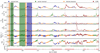 |
Fig. 1. Time series of solar wind parameters for day of year (DoY) 90−150 in 2005. The following solar wind parameters are shown (from top to bottom panel): proton speed vp, proton density np, proton temperature Tp, magnetic field strength B, oxygen charge-state ratio |

Stream interaction regions are sometimes assigned to either of the two slow solar wind types (because most but not all of them are associated with current sheet crossings). For example, the extended interstream region around DoY 101.8−DoY 102.5 (orange shading, no hatching) is here considered as helmet-streamer plasma. Most of the sector-reversal regions are indeed located around changes in the in situ magnetic polarity; an exception is the period from DoY 92.1−94.1 (indicated with dark green shading and hatching), which represents slow solar wind before a stream interaction region without a current sheet crossing2. In general, the sector-reversal category tends to encompass the slowest and densest solar wind.
However, although the Xu & Borovsky (2015) categorization works reliably for the most part, there are some exceptions, and a few of these are highlighted in Fig. 1. For example, according to the categorization, within the second high-speed stream (DoY 102.9−DoY 106.2, blue shading) two streams of the helmet-streamer plasma type appear to be embedded. Because the oxygen charge-state ratio gradually increases throughout the whole time frame, this is not very realistic. Figure 1 also contains examples for potential misidentifications between the two slow solar wind types (helmet-streamer plasma and streamer belt plasma). Within the sector-reversal stream (DoY 98−101.7, dark green shading, no hatching), several short time-frames are instead categorized as helmet-streamer plasma. Similarly, short periods of sector-reversal plasma appear to be embedded in helmet-streamer plasma (DoY 91−DoY 91.7, orange shading with hatching). The latter two examples probably both contradict the concept of assigning a complete solar wind stream to the sector-reversal plasma as long as it contains a change in the magnetic polarity. These occasional misclassifications might be resolved by incorporating charge-state information into the solar wind classification method. However, this is beyond the scope of the Xu & Borovsky (2015) scheme and this work.
Figure 2 shows two-dimensional histograms of the proton-proton collisional age versus the proton speed, proton density, proton temperature, magnetic field strength, B⊥/B as a measure for the wave activity, and the oxygen charge-state ratio  . Each row corresponds to the same solar wind parameter and each column refers to the same solar wind type. The first three columns correspond to sector-reversal plasma, helmet-streamer plasma, and coronal hole wind. The histogram values (indicated by the color bar) in the first three columns are first divided by the respective bin size and then normalized to their corresponding maxima. The fourth column is the sum of the first three (normalized) histograms. This normalization reduces the effect of different underrepresented solar wind types in the fourth column. In each row, the proton-proton collisional age is highest for sector-reversal plasma, has intermediate values for helmet-streamer plasma, and is lowest for coronal hole wind. That the collisional age is lowest for coronal hole wind is expected. Coronal hole wind is typically characterized by a low
  charge-state ratio, high proton speed, low proton density, and high (apparent) proton temperatures. The latter three are all expressed in a low collisional age (see Eq. (1)). That the collisional age is systematically higher in sector-reversal plasma than in helmet-streamer plasma (as is visible in Fig. 2), however, is not immediately obvious from its definition as slow solar wind plasma that contains a current sheet crossing. In the Xu & Borovsky (2015) scheme, many stream interaction boundaries are classified as sector-reversal plasma because they (frequently but not always) contain current sheet crossings. In compression regions in stream interaction regions, the proton density, proton temperature, and magnetic field strength are high (see, e.g., Fig. 1). However, in the compressed slow solar wind, the proton temperature is also higher than in uncompressed slow solar wind. That the proton-proton collisional age is nevertheless higher in this regime than in helmet-streamer plasma indicates that the heating in the compression regions does not completely compensate for the increase in proton density. As the example in Fig. 1 illustrates, not all stream interaction regions and not only stream interaction regions are assigned to the sector-reversal type, however. As illustrated in Fig. 1, the sector-reversal category also contains very slow and dense solar wind with typically low temperatures. All three of these properties also lead to a particularly high proton-proton collisional age.
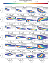 |
Fig. 2. Two-dimensional histograms of logarithmic proton-proton collisional age vs. solar wind parameters. Each histogram is normalized to its maximum value, and each histogram values is divided by the respective bin size before normalization. Each row corresponds to the same solar wind parameter (from top to bottom: proton speed vp, proton density np, proton temperature Tp, magnetic field strength B, perpendicular variability of the magnetic field B⊥/B, and oxygen charge-state ratio |

For the proton density, the proton temperature, the magnetic field strength, and B⊥/B, the fourth column in Fig. 2 shows three visibly separated maxima. This already provides an indication that constant thresholds in the proton-proton collisional age alone (without magnetic field information) appear to be sufficient to distinguish between the three plasma types. This observation motivates us to derive thresholds of constant proton-proton collisional age as an alternative method for distinguishing between the same solar wind types as the Xu & Borovsky (2015) categorization scheme.
4. Solar wind categorized based on proton-proton collisional age
In the following, we describe two alternative approaches for deriving threshold values in the proton-proton collisional age, called similarity-PAC (in Sect. 4.1) and distribution-PAC (in Sect. 4.3). Both variants of the PAC scheme define thresholds in the proton-proton collisional age that aim to separate coronal hole wind, helmet-streamer plasma, and sector-reversal plasma. We refer to the threshold value between coronal hole wind and helmet-streamer plasma as  , and to the threshold value between helmet-streamer plasma and sector-reversal as
  .
.
4.1. Similarity-PAC method and its relation to the Xu & Borovsky (2015) scheme
As a first approach, we varied the positions of the two thresholds  and
and  and computed the similarity of the resulting proton-proton collisional age-based classification scheme to the Xu & Borovsky (2015) scheme. As a similarity measure, we counted the number of data points that were assigned to the same classes for both classification schemes and divided this by the sample size. ICMEs were again excluded from the data set. Figure 3 shows this similarity measure for varying positions of
  and
and  . The highest possible value of this similarity measure is 1, which would be achieved if all data points from all three considered solar wind types were classified the same in both classification schemes. The plus in Fig. 3 indicates the highest observed similarity of 0.90. Because the maximum is comparatively broad, the ranges
 ![Mathematical equation: $ \log\left(a_{{\mathrm{col},\mathrm{p}{\text{-}}\mathrm{p}}}^{\mathrm{ch}}\right)\in[-1.00,-0.95] $](/articles/aa/full_html/2020/04/aa37378-19/aa37378-19-eq17.gif) and
and ![Mathematical equation: $ \log\left(a_{{\mathrm{col},\mathrm{p}{\text{-}}\mathrm{p}}}^{\mathrm{hr}}\right)\in[0.10,0.21] $](/articles/aa/full_html/2020/04/aa37378-19/aa37378-19-eq18.gif) provide reasonable values for the proposed acol, p-p method. In this way, we can derive thresholds for the proton-proton collisional age that result in a categorization that is simimlar to the original Xu & Borovsky (2015) scheme. This represents the first variant of our proposed solar wind classification scheme: the similarity-PAC.
provide reasonable values for the proposed acol, p-p method. In this way, we can derive thresholds for the proton-proton collisional age that result in a categorization that is simimlar to the original Xu & Borovsky (2015) scheme. This represents the first variant of our proposed solar wind classification scheme: the similarity-PAC.
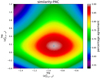 |
Fig. 3. Similarity between the Xu & Borovsky (2015) solar wind types and the similarity-PAC solar wind categorization for different threshold values. The x-axis varies the value of the threshold on the proton-proton collisional age between coronal hole wind and helmet-streamer plasma |


Xu & Borovsky (2015) provided expressions for the decision boundaries in terms of proton speed, proton density, proton temperature, and magnetic field strength. We employed these to express the decision boundaries in terms of the proton-proton collisional age. The first decision boundary (Q1, Eq. (8) in Xu & Borovsky 2015) only separates ejecta from the three other solar wind types. In the following, we therefore only consider the remaining two decision boundaries. Expressing the second and third decision boundaries (Q2: Eq. (9) and Q3: Eq. (10) in Xu & Borovsky 2015) in terms of the proton-proton collisional age yields (after converting everything into the same units)
Notably, these expressions do not directly imply a constant value of the collisional age for each decision boundary, and they depend explicitly on the magnetic field strength, which does not appear in Eq. (1) directly. That constant thresholds in collisional age nevertheless lead to a solar wind classification that is very similar to the full Xu & Borovsky (2015) scheme implies that all information about the magnetic field required for this classification is already encoded in the proton plasma properties. This indicates an additional underlying relationship between the respective quantities that appears to lead to this effect. For the separation between coronal hole wind and helmet-streamer plasma, this can be explained by the expected underlying correlation between proton temperature and magnetic field strength.
4.2. Solar cycle dependence of solar wind parameters
Like the Sun itself, the solar wind properties change with the solar activity cycle (Manoharan 2012; Lepri et al. 2013; Zhao & Fisk 2010; Kasper et al. 2012; Schwadron et al. 2011). Furthermore, Zhao & Landi (2014) showed that the coronal hole wind from equatorial and polar coronal holes has different characteristics (independent of the solar activity cycle). Because small equatorial coronal holes (at low latitudes) are more frequent (but also more short-lived) during solar activity maximum than during solar activity minimum, this alone already implies different properties of a “typical” coronal hole wind in different phases of the solar activity cycle. In the concept of the solar wind described by Antiochos et al. (2011), all coronal holes are connected. Here, the differences between polar and equatorial coronal holes can be understood as a systematic change in solar wind properties with distance to the coronal hole border (see Peleikis et al. 2016).
Figure 4 shows time series of solar wind proton speed, proton density, proton temperature, magnetic field strength, perpendicular variability of the magnetic field B⊥/B, Alfvén speed, specific proton entropy, the ratio of observed proton temperature to the expected temperature, the proton-proton collisional age, and the monthly sunspot number (from version 2.0 of the SILSO data, Royal Observatory of Belgium, Brussels, Clette et al. 2016). Except for the last panel, each panel shows data for coronal hole wind, helmet-streamer plasma, and sector-reversal plasma, and each data point is averaged over the entire solar wind of the respective type from one synodic solar rotation. We assumed an approximate length of a Carrington rotation of 27.24 days and used this as the bin size. The true start point of the Carrington rotation was ignored. As observed in Manoharan (2012), Lepri et al. (2013), Zhao & Fisk (2010), Kasper et al. (2012), and Schwadron et al. (2011), most of these solar wind parameters change systematically following the solar activity cycle. In particular, the magnetic field strength and the oxygen charge-state ratio (panels 4 and 5) exhibit lower values during the solar activity minimum than during the solar activity maximum. This holds for each of the three solar wind types separately. Oxygen charge state ratios that are associated with coronal hole wind during the solar activity maximum would fall in the range of slow solar wind if they were observed during the solar activity minimum. A similar but weaker trend is also observed for proton speed, proton temperature, and proton density. This emphasizes that solar wind categorization based on thresholds in both charge state compositions and proton plasma properties cannot be expected to perform equally well in all phases of the solar activity cycle with the same fixed threshold values. Instead, the thresholds need to be dependent on the phase of the solar activity cycle.
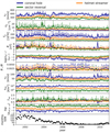 |
Fig. 4. Time series of solar wind parameters averaged over 27.24 days and separated by solar wind type in the Xu & Borovsky (2015) scheme within each time bin. From top to bottom: proton speed vp, proton density n, proton temperature Tp, magnetic field strength B, oxygen charge-state ratio |

For the whole time frame shown in Fig. 4, the values of the collisional age and the specific proton entropy for the three plasma types are well separated. However, because the solar wind types in Fig. 4 are based on the fixed Xu & Borovsky (2015) scheme that does not reflect, for example, overall lower proton densities and magnetic field strength during the solar activity minimum, the temporal variation is probably underestimated. This also means that for the collisional age and the specific proton entropy, the same fixed thresholds cannot (yet) be expected to be the optimal choice throughout the whole solar activity cycle. The separation between the different solar wind types shown in Fig. 4 indicates that the specific proton entropy and the proton-proton collisional age are best suited as single parameters in a one-dimensional solar wind categorization scheme. It should be noted that a large overlap between the different solar wind types in Fig. 4 only rules out the respective parameter for a one-dimensional classification scheme. The informative value of these parameters in a higher dimensional decision space cannot be estimated in this representation.
4.3. Time-dependent solar wind classification based on the proton-proton collisional age
Based on the considerations in the previous section, we derive a second, time-dependent criterion for threshold values in the proton-proton collisional age. Under the assumption that all three solar wind types are well represented in the data set, this approach is based directly on the distribution of the proton-proton collisional age and is therefore called the distribution-PAC method. To ensure reasonable statistics, we divided the time series into batches of 6 × 27.24 days (corresponding to six times the approximate length of a Carrington rotation). Figure 5 shows normalized one-dimensional histograms of the proton-proton collisional age for the first 163.44 days in 2001, 2005, and 2009. To reduce the effect of unbalanced samples for each of the three solar wind types, each solar wind type (for illustrative purposes, the Xu & Borovsky 2015 types are used here again) is binned separately and is normalized to its respective maximum. The lower panels for each year in Fig. 5 show these normalized histograms. Then, the minima between the two class pairs (sector-reversal plasma and helmet-streamer plasma on the one hand, and helmet-streamer plasma and coronal hole wind on the other) are taken as the new estimate for the threshold values. In all three subplots, a tail at log acol, p-p ∼ 1 is visible. In 2001, this population is frequent enough to form an additional peak. This is probably related to ICMEs that are missing from the ICME lists or ICMEs whose start and end times are too inaccurate in the ICME lists. However, when we use the Xu & Borovsky (2015) solar wind classification as a starting point, as in Fig. 5, this approach requires a ground truth for the solar wind categorization as prior information. To avoid this, we used an iterative random search that is illustrated in Fig. 6: Step 1: For each time frame a one-dimensional histogram of the proton-proton collisional age is generated. Step 2: An initial guess ( and
and  modified with additive uniform noise in [ − 0.1, 0.1]) provides candidates for the decision boundaries. Step 3: Based on these thresholds, a candidate classification is derived. Step 4: Each of these candidate solar wind types is separately normalized by its maximum. Step 5: From the sum of these normalized histograms, new thresholds are derived as the minima between the two main peaks. To increase robustness against noise and underrepresented solar wind types, the two main peaks are required to be in acol, p-p ∈ [ − 1.5, 0.8]. Step 6: The derived thresholds are evaluated by adding the histogram values at the minima. These six steps are then repeated 10 000 times. We take the result that leads to the deepest minima in the renormalized histogram as the final solution. This approach assumes that at least three solar wind types are always present in the data. The approach is otherwise purely data-driven. This process is then applied to each data batch (with a length of 6 × 27.24 days), and the results are shown in Fig. 7.
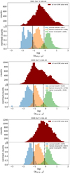 |
Fig. 5. Summed 1-dimensional histograms of the proton-proton collisional age for different selected time frames. Top: DoY 1−164.44 in 2001. Middle: 1−164.44 in 2005. Bottom: DoY 1−164.44 in 2009. In each subplot, the upper panel gives the non-normalized histograms of all observations for the three solar wind types (coronal hole wind in dark blue, helmet-streamer plasma in orange, and sector-reversal plasma in dark green, following the Xu & Borovsky 2015 scheme), the lower panel shows the three histograms normalized according to solar wind type. The black solid vertical lines indicate the respective minimum |


In this figure, two pairs of threshold values are given: thresholds between coronal hole wind and helmet-streamer plasma (lower lines at  , solid lines), and thresholds between helmet-streamer plasma and sector-reversal plasma (upper lines at
  , dashed lines). The blue lines refer to the similarity-PAC method and are derived based on the similarity to the Xu & Borovsky (2015) scheme, as described in Sect. 4.1. The only difference to Sect. 4.1 is that the method is here also applied to the 6 × 27.24 time bins. The black lines represent the results of the distribution-PAC approach derived from the proton-proton collisional age distribution as described in this section and illustrated in Fig. 6.
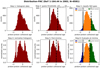 |
Fig. 6. Distribution-PAC method for one time frame (DoY 1−164.44 in 2002). Each panels shows one-dimensional histograms of the proton-proton collisional age. In the second row, all histograms are normalized to their respective maxima. Solid and dashed vertical lines indicate classification thresholds. The circles in the last panel in the second row indicate the histogram values used for the evaluation of the candidate solution. The sample size N is given in the figure title. |
Consecutively applied to data batches, both criteria (the similarity to the Xu & Borovsky 2015 scheme and the distribution-based approach) lead to time-variable thresholds. However, the thresholds derived from both criteria (similarity-PAC and distribution-PAC) show comparatively small variations throughout the solar cycle, wherein distribution-PAC exhibits slightly larger variations. For the similarity-PAC this might arise because the Xu & Borovsky (2015) scheme fixed separating hyperplanes throughout the solar activity cycle.
The second criterion, the distribution-PAC, directly depends on the observed solar wind mixture. As shown in Fig. 8 (which provides an overview of the relative frequencies of the considered solar wind types over time), a higher fraction of coronal hole wind has been observed in 2003 than in any other year. At the same time, a very low fraction of sector-reversal plasma has been observed. In 2009, a very low fraction of coronal hole wind is observed. Both time frames violate the underlying assumption of our approach that three types of solar wind are always observed with a sufficient relative frequency. Nevertheless, distribution-PAC is able to provide stable classification thresholds. For the similarity-PAC and distribution-PAC, Fig. 7 shows no clear trend with the solar activity cycle. This means that the variability of the threshold values caused by the time-varying mix of solar wind types is probably larger than the variability of the proton-proton collisional age with the solar activity cycle itself.
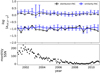 |
Fig. 7. Thresholds in proton-proton collisional age over time derived from the similarity-PAC (solid and dashed blue) and with the distribution-PAC (solid and dashed black). The dashed lines indicate the separation threshold |


Table 1 provides the threshold value for each time frame from Fig. 7. The confidence intervals (in Table 1 and Fig. 7) indicate how far the thresholds can be shifted in any direction at most while changing the occurrence frequency of the predicted solar wind type by at most 5% of the data. The distribution-based method relies on the assumption that all three solar wind types are represented in any given data set. An estimate for this is included in Table 1 (last column): We take the minimum ratio of the numbers of observations from each neighboring pair of solar wind (coronal hole wind versus helmet-streamer plasma, and helmet-streamer plasma versus sector-reversal plasma) in the Xu & Borovsky (2015) scheme as an indicator of how underrepresented the least frequently observed solar wind type is during each time frame. If all three solar wind types were equally frequent in a given data sample, then this reliability parameter would be one. The lower this value, the more unbalanced the data set. As expected from Fig. 8, in 2003 and 2009, the data set suffers most from underrepresentation (sector-reversal plasma is underrepresented in 2003, and coronal hole wind is underrepresented in 2009).
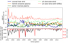 |
Fig. 8. Upper panel: ratio of observations of solar wind types (based on the Xu & Borovsky 2015 scheme) relative to the entire solar wind (without ICMEs) over time (in time bins of length 27.24 days): the entire solar wind with ICMEs, coronal hole wind, helmet-streamer plasma, sector-reversal plasma, and the sum of the two slow solar wind types (entire slow solar wind). Lower panel: number of solar wind observations per time bin and data coverage. |
Classification thresholds derived from distribution of proton-proton collisional age in 163.44 days time resolution.
4.4. Proton plasma solar wind classification without a magnetometer: the distribution-PAC method applied to SOHO
As long as the assumption is valid that the observed solar wind covers all three considered solar wind types, the proposed distribution-PAC approach can be applied to other instruments (and other positions in the heliosphere). As a test case, we applied this method to the plasma data obtained from the proton monitor (PM). The PM is an auxiliary instrument to the mass time-of-flight (MTOF) sensor that is part of the charge, element, and isotope analysis system (CELIAS, Hovestadt et al. 1995) on board the Solar and Heliospheric Observatory (SOHO). We chose SOHO as a test case because both SOHO and ACE are located close to L1 during the time frame shown in Figs. 1 and 9. Therefore we can expect that both spacecraft observe similar solar wind streams. Because SOHO is not equipped with a magnetometer, the full Xu & Borovsky (2015) scheme cannot be applied directly. An example of the resulting solar wind classification is shown in Fig. 9. As the for full Xu & Borovsky (2015) scheme based on ACE data for the same time frame (see Fig. 1), this simple method also leads to some misclassifications. For the most part, however, the solar wind classification behaves as expected: Sector-reversal plasma is mainly concentrated before and during stream interaction regions, and hot, fast, and thin solar wind streams are categorized as coronal hole wind.
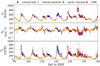 |
Fig. 9. Proton plasma properties from SOHO/CELIAS/MTOF/PM. The colors indicate the solar wind type according to the distribution-PAC criterion (derived only from SOHO/CELIAS/MTOF/PM data): dark blue shows the coronal hole wind, orange represents helmet-streamer plasma, and dark green is used for sector-reversal plasma. |
5. Discussion and conclusion
We find that the proton-proton collisional age alone is similarly well suited to identify the solar wind type as the full Xu & Borovsky (2015) scheme. This is not a direct consequence of the decision boundaries from Xu & Borovsky (2015), but implies an underlying relationship between the magnetic field strength and the proton plasma properties in the solar wind. This relationship is an inherent consequence of the different plasma properties in coronal hole wind and slow solar wind. Typical coronal hole wind properties result in a low proton-proton collisional age, whereas the typical properties in the slow solar wind are expressed in a higher proton-proton collisional age. Although not shown here, ICMEs are also typically associated with high proton-proton collisional ages (because the proton temperature tends to be particularly low and the proton density high). However, from our point of view, ICMEs cannot be separated from sector-reversal plasma with the proton-proton collisional age alone. In general, context information is required to correctly and uniquely identify ICMEs. Outside of ICMEs, sector-reversal plasma (which includes compressed slow solar wind around current sheet crossings) shows the highest proton-proton collisional age. These regions are also characterized by a higher magnetic field strength. This is not directly encoded in the proton-proton collisional age. That the proposed simplified classification scheme based on the proton-proton collisional age (PAC) nevertheless leads to a classification that is very similar to the full Xu & Borovsky (2015) scheme (which has decision boundaries that depend on the magnetic field strength) indicates that all required information about the magnetic field strength is already encoded in the proton plasma properties.
The clear separation visible in the proton-proton collisional age between coronal hole wind and slow solar wind is probably sharpened by the respective presence and absence of wave activity. Wave activity together with a high Alfvén velocity in coronal hole wind leads to (apparent) heating of the solar wind and thus to a further decrease in proton-proton collisional age. That the proton-proton collisional age also separates helmet-streamer and sector-reversal plasma is probably a combination of two effects: the sector-reversal plasma tends to include the densest and slowest slow solar wind streams and in addition contains most of the slow solar wind compression regions. Both types of plasma are characterized by a particularly high collisional age. The collisional age is interpreted as a measure of the history of a particular solar wind plasma package. Computing the proton-proton collisional age based on the in situ proton plasma properties implies the assumption that these conditions affect the solar wind during its complete travel time. However, this assumption is violated in stream interaction regions that become increasingly more frequent and extended farther away from the Sun. In this case, the proton-proton collisional age as considered here therefore overestimates the effect of collisions. For the sake of categorizing the solar wind based on the proton-proton collisional age, this turns out to be beneficial because it increases the differences between helmet-streamer and sector-reversal plasma. The collisional thermalization of the solar wind as described in Maruca et al. (2013) presents an alternative that avoids this ambiguity. Instead of assuming fixed values for the solar wind proton speed, density, and temperature, Maruca et al. (2013) allowed for a radial evolution of these quantities. However, this requires a model for the radial evolution.
We proposed two variants of our categorization of the solar wind based on proton-proton collisional age: similarity-PAC, which is based on the observed similarity to the Xu & Borovsky (2015) scheme, and distribution-PAC, which is a purely data-driven categorization of the solar wind that only relies on the assumption that sufficiently frequent observations from the three solar wind types are contained in the data.
Because the Sun induces systematic changes in the solar wind properties during its solar activity cycle, any solar wind categorization scheme depending on solar wind composition or proton plasma properties should reflect this by featuring thresholds that depend on the solar cycle. Nevertheless, for our PAC schemes, the derived thresholds are more sensitive to the time-varying mixture of solar wind types than to systematic changes in solar wind properties of each solar wind type with the solar activity cycle.
An advantage of the proposed collisional age approach is that the categorization scheme does not require magnetic field measurements, but only proton speed, proton density, and proton temperature. Unlike the full scheme of Xu & Borovsky (2015), the PAC method can be directly applied to observations from the proton monitor on SOHO. A drawback of this approach (and all solar wind categorization schemes that are based on proton plasma properties in general) is that the separating hyperplanes depend on radius and therefore can only be applied at 1 AU in their current form.
This is the only time in this manuscript that eV and not K is used as unit for the temperature.
Polarity changes on scales of single or a few data points in the 12 min time resolution are not necessarily associated with crossings of the heliospheric current sheet, but are most likely caused by localized kinks in the magnetic field (Berger et al. 2011). These are therefore not indications of misclassifications between helmet-streamer and sector-reversal plasma.
Acknowledgments
Part of this work was supported by the Deutsche Forschungsgemeinschaft (DFG) project number Wi-2139/11-1. We further thank the science teams of ACE/SWEPAM, ACE/MAG as well as ACE/SWICS for providing the respective level 2 and level 1 data products. We gratefully acknowledge the diligent and detailed work of the referee.
References
- Antiochos, S., Mikić, Z., Titov, V., Lionello, R., & Linker, J. 2011, ApJ, 731, 112 [Google Scholar]
- Bale, S., Badman, S., Bonnell, J., et al. 2019, Nature, 576, 237 [NASA ADS] [CrossRef] [Google Scholar]
- Berger, L. 2008, PhD Thesis, Kiel, Christian-Albrechts-Universität, Diss. [Google Scholar]
- Berger, L., Wimmer-Schweingruber, R., & Gloeckler, G. 2011, Phys. Rev. Lett., 106, 151103 [NASA ADS] [CrossRef] [Google Scholar]
- Camporeale, E., Carè, A., & Borovsky, J. E. 2017, J. Geophys. Res.: Space Phys., 122, 10 [Google Scholar]
- Cane, H., & Richardson, I. 2003, J. Geophys. Res.: Space Phys., 108, A4 [CrossRef] [Google Scholar]
- Clette, F., Lefèvre, L., Cagnotti, M., Cortesi, S., & Bulling, A. 2016, Sol. Phys., 291, 2733 [Google Scholar]
- D’Amicis, R., & Bruno, R. 2015, ApJ, 805, 84 [NASA ADS] [CrossRef] [Google Scholar]
- Gloeckler, G., Cain, J., Ipavich, F., et al. 1998, The Advanced Composition Explorer Mission (Springer), 497 [Google Scholar]
- Heidrich-Meisner, V., & Wimmer-Schweingruber, R. F. 2018, Machine Learning Techniques for Space Weather (Elsevier), 397 [Google Scholar]
- Hovestadt, D., Hilchenbach, M., Bürgi, A., et al. 1995, Sol. Phys., 162, 441 [NASA ADS] [CrossRef] [Google Scholar]
- Jian, L., Russell, C., Luhmann, J., & Skoug, R. 2006, Sol. Phys., 239, 393 [NASA ADS] [CrossRef] [Google Scholar]
- Jian, L., Russell, C., & Luhmann, J. 2011, Sol. Phys., 274, 321 [NASA ADS] [CrossRef] [Google Scholar]
- Kasper, J., Lazarus, A., & Gary, S. 2008, Phys. Rev. Lett., 101, 261103 [NASA ADS] [CrossRef] [PubMed] [Google Scholar]
- Kasper, J., Stevens, M., Korreck, K., et al. 2012, ApJ, 745, 162 [NASA ADS] [CrossRef] [Google Scholar]
- Kasper, J., Bale, S., Belcher, J., et al. 2019, Nature, 576, 1 [Google Scholar]
- Lepri, S., Landi, E., & Zurbuchen, T. 2013, ApJ, 768, 94 [NASA ADS] [CrossRef] [Google Scholar]
- Lin, R., Anderson, K., Ashford, S., et al. 1995, Space Sci. Rev., 71, 125 [NASA ADS] [CrossRef] [Google Scholar]
- Manoharan, P. 2012, ApJ, 751, 128 [NASA ADS] [CrossRef] [Google Scholar]
- Marsch, E., Mühlhäuser, K.-H., Schwenn, R., et al. 1982, J. Geophys. Res.: Space Phys., 87, 52 [NASA ADS] [CrossRef] [Google Scholar]
- Maruca, B. A., Bale, S. D., Sorriso-Valvo, L., Kasper, J. C., & Stevens, M. L. 2013, Phys. Rev. Lett., 111, 241101 [NASA ADS] [CrossRef] [Google Scholar]
- McComas, D., Bame, S., Barker, P., et al. 1998, The Advanced Composition Explorer Mission (Springer), 563 [CrossRef] [Google Scholar]
- McComas, D., Barraclough, B., Funsten, H., et al. 2000, J. Geophys. Res.: Space Phys., 105, 10419 [NASA ADS] [CrossRef] [Google Scholar]
- Peleikis, T., Kruse, M., Berger, L., Drews, C., & Wimmer-Schweingruber, R. F. 2016, AIP Conf. Ser., 1720, 020003 [Google Scholar]
- Richardson, I., & Cane, H. 2010, Sol. Phys., 264, 189 [NASA ADS] [CrossRef] [Google Scholar]
- Sanchez-Diaz, E., Rouillard, A. P., Lavraud, B., et al. 2016, J. Geophys. Res.: Space Phys., 121, 2830 [NASA ADS] [CrossRef] [Google Scholar]
- Schwadron, N., Smith, C., Spence, H. E., et al. 2011, ApJ, 739, 9 [NASA ADS] [CrossRef] [Google Scholar]
- Smith, C. W., L’Heureux, J., Ness, N. F., et al. 1998, The Advanced Composition Explorer Mission (Springer), 613 [CrossRef] [Google Scholar]
- Stakhiv, M., Landi, E., Lepri, S. T., Oran, R., & Zurbuchen, T. H. 2015, ApJ, 801, 100 [NASA ADS] [CrossRef] [Google Scholar]
- Tracy, P. J., Kasper, J. C., Raines, J. M., et al. 2016, Phys. Rev. Lett., 116, 255101 [NASA ADS] [CrossRef] [Google Scholar]
- von Steiger, R., Schwadron, N., Fisk, L., et al. 2000, J. Geophys. Res., 105, 27 [Google Scholar]
- Wilson, L. B., III, Stevens, M. L., Kasper, J. C., et al. 2018, ApJS, 236, 41 [NASA ADS] [CrossRef] [Google Scholar]
- Xu, F., & Borovsky, J. E. 2015, J. Geophys. Res.: Space Phys., 120, 70 [NASA ADS] [CrossRef] [Google Scholar]
- Zhao, L., & Fisk, L. 2010, SOHO-23: Understanding a Peculiar Solar Minimum, 428, 229 [NASA ADS] [Google Scholar]
- Zhao, L., & Landi, E. 2014, ApJ, 781, 110 [NASA ADS] [CrossRef] [Google Scholar]
All Tables
Classification thresholds derived from distribution of proton-proton collisional age in 163.44 days time resolution.
All Figures
|
Fig. 1. Time series of solar wind parameters for day of year (DoY) 90−150 in 2005. The following solar wind parameters are shown (from top to bottom panel): proton speed vp, proton density np, proton temperature Tp, magnetic field strength B, oxygen charge-state ratio |
| In the text | |
|
Fig. 2. Two-dimensional histograms of logarithmic proton-proton collisional age vs. solar wind parameters. Each histogram is normalized to its maximum value, and each histogram values is divided by the respective bin size before normalization. Each row corresponds to the same solar wind parameter (from top to bottom: proton speed vp, proton density np, proton temperature Tp, magnetic field strength B, perpendicular variability of the magnetic field B⊥/B, and oxygen charge-state ratio |
| In the text | |
|
Fig. 3. Similarity between the Xu & Borovsky (2015) solar wind types and the similarity-PAC solar wind categorization for different threshold values. The x-axis varies the value of the threshold on the proton-proton collisional age between coronal hole wind and helmet-streamer plasma |
| In the text | |
|
Fig. 4. Time series of solar wind parameters averaged over 27.24 days and separated by solar wind type in the Xu & Borovsky (2015) scheme within each time bin. From top to bottom: proton speed vp, proton density n, proton temperature Tp, magnetic field strength B, oxygen charge-state ratio |
| In the text | |
|
Fig. 5. Summed 1-dimensional histograms of the proton-proton collisional age for different selected time frames. Top: DoY 1−164.44 in 2001. Middle: 1−164.44 in 2005. Bottom: DoY 1−164.44 in 2009. In each subplot, the upper panel gives the non-normalized histograms of all observations for the three solar wind types (coronal hole wind in dark blue, helmet-streamer plasma in orange, and sector-reversal plasma in dark green, following the Xu & Borovsky 2015 scheme), the lower panel shows the three histograms normalized according to solar wind type. The black solid vertical lines indicate the respective minimum |
| In the text | |
|
Fig. 6. Distribution-PAC method for one time frame (DoY 1−164.44 in 2002). Each panels shows one-dimensional histograms of the proton-proton collisional age. In the second row, all histograms are normalized to their respective maxima. Solid and dashed vertical lines indicate classification thresholds. The circles in the last panel in the second row indicate the histogram values used for the evaluation of the candidate solution. The sample size N is given in the figure title. |
| In the text | |
|
Fig. 7. Thresholds in proton-proton collisional age over time derived from the similarity-PAC (solid and dashed blue) and with the distribution-PAC (solid and dashed black). The dashed lines indicate the separation threshold |
| In the text | |
|
Fig. 8. Upper panel: ratio of observations of solar wind types (based on the Xu & Borovsky 2015 scheme) relative to the entire solar wind (without ICMEs) over time (in time bins of length 27.24 days): the entire solar wind with ICMEs, coronal hole wind, helmet-streamer plasma, sector-reversal plasma, and the sum of the two slow solar wind types (entire slow solar wind). Lower panel: number of solar wind observations per time bin and data coverage. |
| In the text | |
|
Fig. 9. Proton plasma properties from SOHO/CELIAS/MTOF/PM. The colors indicate the solar wind type according to the distribution-PAC criterion (derived only from SOHO/CELIAS/MTOF/PM data): dark blue shows the coronal hole wind, orange represents helmet-streamer plasma, and dark green is used for sector-reversal plasma. |
| In the text | |
Current usage metrics show cumulative count of Article Views (full-text article views including HTML views, PDF and ePub downloads, according to the available data) and Abstracts Views on Vision4Press platform.
Data correspond to usage on the plateform after 2015. The current usage metrics is available 48-96 hours after online publication and is updated daily on week days.
Initial download of the metrics may take a while.