| Issue |
A&A
Volume 693, January 2025
|
|
|---|---|---|
| Article Number | A191 | |
| Number of page(s) | 8 | |
| Section | The Sun and the Heliosphere | |
| DOI | https://doi.org/10.1051/0004-6361/202452845 | |
| Published online | 17 January 2025 | |
Challenges in identifying the coronal hole wind
1
Christian Albrechts University, Kiel, Germany
2
TUD Dresden University of Technology, Dresden, Germany
⋆ Corresponding author; This email address is being protected from spambots. You need JavaScript enabled to view it.
Received:
1
November
2024
Accepted:
15
December
2024
Abstract
Context. Solar wind is frequently categorized based on its respective solar source region. Solar wind that originates in coronal holes is consequently called coronal hole wind. Two well-established categorizations of the coronal hole wind, the scheme based on the charge-state composition, and the scheme based on proton plasma, identify a very different fraction of solar wind in the data from the Advanced Composition Explorer (ACE) as coronal hole wind during the solar activity minimum at the end of solar cycle 24.
Aims. We investigate possible explanations for the different identifications of the coronal wind in 2009 in the scheme based on the charge-state composition (almost only coronal hole wind) and in the scheme based on the proton plasma (almost no coronal hole wind at the same time). The high fraction of coronal hole wind observed in the scheme based on the charge-state composition in 2009 was also addressed previously.
Methods. We compared the properties of the respective coronal hole wind types and their changes with solar activity cycle in 2001–2010. As a comparison reference, we included the coronal hole wind as identified by an unsupervised machine-learning approach, k-means, in our analysis.
Results. Because the ratio of the O7+ to O6+ densities drops systematically for the entire solar wind during the solar activity minimum, which cannot be captured by the fixed threshold on the O charge-state ratio suggested in the scheme based on the charge-state composition, we find that this solar wind classification likely misidentifies some slow solar wind as coronal hole wind during the solar activity minimum. The k-means coronal hole wind agrees with the very low fraction of coronal hole wind observed in the classification based on the proton plasma. In addition, the k-means classification we considered includes two types of coronal hole wind, the first of which is dominant during the solar activity maximum and exhibits comparatively higher O and Fe charge states, whereas the second is dominant during the solar activity minimum and features lower O and Fe charge states. A low fraction of coronal hole wind from low-latitude coronal holes observed by ACE in 2009 is plausible because during this time period, a very small number of low-latitude coronal holes was observed. The scheme based on proton plasma and 7-means also relies on fixed decision boundaries, wherein the decision boundary in the scheme based on the proton plasma for coronal hole wind appears to be better adapted for conditions at solar activity minimum than maximum.
Conclusions. The results imply that the origin-oriented solar wind classification needs to be revisited, and they also suggest that an explicit inclusion of the phase of the solar activity cycle can be expected to improve the classification of the solar wind.
Key words: Sun: heliosphere / solar wind
© The Authors 2025
 Open Access article, published by EDP Sciences, under the terms of the Creative Commons Attribution License (https://creativecommons.org/licenses/by/4.0), which permits unrestricted use, distribution, and reproduction in any medium, provided the original work is properly cited.
This article is published in open access under the Subscribe to Open model. This email address is being protected from spambots. You need JavaScript enabled to view it. to support open access publication.
1. Introduction
The solar wind is the plasma that is continuously emitted by the Sun. It has been investigated for several decades (Parker 1965; Marsch 2006; Cranmer 2009; Verscharen et al. 2019; Vidotto 2021). The properties of the solar wind depend on the conditions in the corona at its solar source region and are modified by transport effects. The best-understood flavor of solar wind is called coronal hole wind because its source region was identified as coronal holes (Hundhausen et al. 1968; Krieger et al. 1973; Tu et al. 2005; Cranmer 2009). Compared to the so-called slow solar wind, coronal hole wind is considered to be better understood (Cranmer 2009). Recently, the release mechanism of coronal hole wind has been linked to interchange reconnection (Bale et al. 2023) and picoflares (Chitta et al. 2023). Zhao & Landi (2014) showed that the properties of coronal hole wind from polar coronal holes differ from those from equatorial coronal holes. This effect is correlated to the footpoint field strength in the respective coronal hole (Wang & Ko 2019; D’Amicis et al. 2019; D’Amicis et al. 2021; Bale et al. 2019; Stansby et al. 2019; Wang 2024).
The coronal hole wind is a collisionless plasma, and, therefore, nonthermal features play an important role in its properties. Waves are frequently observed in coronal hole wind (Marsch et al. 1982a; D’Amicis & Bruno 2015). Wave-particle interactions lead to various interesting features in coronal hole wind, for example, a proton beam (Marsch et al. 1982b), differential streaming between protons and heavier ions Marsch et al. (1981), Berger et al. (2011), and temperature anisotropies (Marsch et al. 2006; Kasper et al. 2003; Huang et al. 2020). The variety of its nonthermal features make coronal hole wind an interesting object of study (see, e.g., the role of the Alfvéincity parameter in D’Amicis et al. 2019; D’Amicis et al. 2021; Bale et al. 2019; Stansby et al. 2019), even though its solar source region is comparatively well understood.
To study solar wind from different solar sources separately, a classification of the solar wind is often employed. The most prominent solar wind classification approaches focus on determining the respective solar source region (Zhao et al. 2009; Xu & Borovsky 2015; Camporeale et al. 2017). More recently, unsupervised machine-learning approaches were applied to categorize the solar wind (Bloch et al. 2020; Heidrich-Meisner & Wimmer-Schweingruber 2018; Amaya et al. 2020). In these data-driven methods, more solar wind types are identified that represent a mixture of source and transport-affected properties. In the following, we use a k-means solar wind classification as a data-driven reference classification. k-means was chosen here because similar to Zhao et al. (2009) and Xu & Borovsky (2015), k-means relies on fixed decision boundaries.
Neugebauer et al. (2016) showed that although established solar wind categorizations agree on the basic types of solar wind, they disagree on how exactly the boundaries are defined. To the best of our knowledge, a ground truth for the solar wind categorization is still not available.
We focus on the coronal hole wind identified by three different solar wind categorizations, the scheme based on charge-state composition Zhao et al. (2009), that based on the proton-plasma property Xu & Borovsky (2015), and an unsupervised machine-learning approach, k-means similar to Bloch et al. (2020) and Heidrich-Meisner & Wimmer-Schweingruber (2018). Based on Heidrich-Meisner & Wimmer-Schweingruber (2018), k = 7 was chosen as a reference case for this study. Our study is motivated by the very different fractions of coronal hole wind identified by these three approaches. This is illustrated in Fig. 1, which shows for each of the three categorizations the varying fractions of solar wind types observed by the Advanced Composition Explorer (ACE) in 2001–2010. The most striking difference occured in 2009 during the solar activity minimum. The scheme based on the composition Zhao et al. (2009) here identifies almost the entire solar wind as coronal hole wind, while the scheme by Xu & Borovsky (2015) detects almost no coronal hole wind in the same time period. The unsupervised machine-learning approach, 7-means, includes two types of coronal hole wind, and both of them make up only a small fraction of the solar wind observed in 2009. This figure is discussed in more detail in Sect. 4 after an overview of the underlying data set in Sect. 2.1 and the three solar wind categorizations of interest in Sect. 3. The high fraction of coronal hole wind identified by the Zhao et al. (2009) approach was already discussed in detail in Wang (2016), Wang & Ko (2019), who showed that the O charge-state composition is related to the footpoint magnetic field strength at the likely source region. We focus on the comparison with the other coronal hole wind characterizations and on explanations of which solar wind parameters contribute to the identification of coronal hole wind.
 |
Fig. 1. Fractions of solar wind types from three solar wind classifications per three Carrington rotations. From left to right: (a) Zhao et al. (2009), (b) Xu & Borovsky (2015), and (c) 7-means clustering. The green shading highlights 2009. All noncoronal hole wind types (Panel a): Slow and ICME. Panel (b): Sector-reversal, helmet streamer, and ejecta. Panel (c): Remaining five types identified by 7-means (numbered as types T1, ..., T5) are shown in different shades of gray to keep the focus on the coronal hole wind types of interest. |
2. Data and methods
In this section, we briefly describe the data and methods. We describe all preprocessing steps in Sect. 2.1. An explainability tool used in Sect. 4 is introduced in more detail in Sect. 2.2.
2.1. Data
Our aim is to compare coronal hole wind types identified by different solar wind categorizations that in part rely on the charge-state composition. To do this, we used data observed by three instruments on ACE: the magnetic field strength B from the magnetometer (MAG; Smith et al. 1998), the proton speed vp, proton density np, and proton temperature Tp from the Solar Wind Electron Proton Alpha Monitor (SWEPAM; McComas et al. 1998), and the heavy ion charge-state composition (ratio of the O7+ density to the O6+ density  and the average Fe charge-state
  based on the Fe8+ – Fe13+ Fe charge states) from the Solar Wind Ion Composition Spectrometer (SWICS; Gloeckler et al. 1998). To ensure a minimum of statistics, the average Fe charge was only considered if at least ten Fe ions were observed. We verified that the results did not change systematically when this threshold was modified. We chose a low threshold since the higher the threshold, the stronger the selection bias toward a denser solar wind. This bias is expected to reduce the number of available data points in particular for coronal hole wind from polar coronal holes during solar activity minimum conditions. The low threshold thus represents a compromise between sufficient statistics for the determination of the charge-state distributions and the number of available data points to which we can apply our analysis. The MAG and SWEPAM data were binned to the native 12 min time resolution of SWICS. To avoid data gaps in the SWEPAM data, the merged SWEPAM-SWICS data set was used. The MAG and SWEPAM data sets were taken from the ACE Science Center. Interplanetary coronal mass ejections (ICMEs) were independently taken from published ICME lists (Jian et al. 2006, 2011; Cane & Richardson 2003; Richardson & Cane 2010). As a derived parameter, we considered the proton-proton collisional age (also called Coulomb number in Kasper et al. 2012). As discussed in Heidrich-Meisner et al. (2020), the proton-proton collisional age is well suited for a reconstruction of the Xu & Borovsky (2015) solar wind types. The relevant part of the data set is available at Berger et al. (2023). The heavy ion composition was derived from the pulse-height-analysis (PHA) words as described in Berger (2008).
2.2. Feature explanations
In Sect. 4 we employ a machine-learning tool to illustrate and analyze the differences between the four coronal hole wind types of interest. In recent years, the concept of explainability has gained attention in the machine-learning community (see, e.g., Solorio-Fernández et al. 2020; Kumar & Minz 2014; Alelyani et al. 2018). In contrast to black-box results, explainability in this context refers to tools that provide interpretable explanations for the results of a machine-learning method. Some of these tools, in particular, posthoc explainability concepts such as Shapley additive explanations (SHAP; Lundberg & Lee 2017) values, can also be applied to non-machine-learning approaches. SHAP values are based on Shapeley values (Shapley 1953) that were originally designed for ranking players in collaborative games with teams of varying sizes. Lundberg & Lee (2017) proposed to apply Shapely values to explainability by interpreting the input parameters, in our case, the solar wind properties (vp, np, Tp, B, acol, p − p,  , and
, and  ), as individual players in such a collaborative game. Teams of players then represent combinations of several input parameters. SHAP values can only be applied to regression or binary classification tasks directly. We applied this concept to binary classification. Therefore, we treated the identification of coronal hole wind by each of the classifications as a binary classification task wherein a value of one represents the respective coronal hole wind type, and a value of zero represents any other solar wind type.
The SHAP values then quantify how important each player, that is, each solar wind parameter, is to win the game. In this context, “winning1” corresponds to identifying data points as coronal hole wind. High (positive) SHAP values then indicate solar wind properties that are important for identifying data points as coronal hole wind, whereas negative SHAP values with high absolute values indicate solar wind parameters that are important for identifying non-coronal hole wind. SHAP values close to zero always represent unimportant parameters. In this study, we focus on positive SHAP values. The SHAP values were computed for each data point separately. An overall importance of each feature can be obtained by summing all respective SHAP values. We are interested in the change in the importance of the respective solar wind parameters over time, and we therefore computed the SHAP values for each Carrington rotation separately. In addition to assessing the importance of solar wind parameters above or below the respective median value, the SHAP values for solar wind parameters above the median and below the median are represented separately. The SHAP values assess the importance of single parameters and provide no information on the importance of tuples of input parameters.
3. Approaches to classifying coronal hole wind
In this study, we consider three solar wind classification approaches:
-
The scheme based on the charge-state composition Zhao et al. (2009) distinguishes between coronal hole wind and slow solar wind with a fixed threshold on the O charge-state ratio
 and identifies all solar wind with
  as coronal hole wind. ICMEs are distinguished from the slow solar wind based on the proton speed vp.
 -
The scheme based on the proton plasma Xu & Borovsky (2015) defines fixed decision boundaries based on the Alfvén speed vA, the specific proton entropy Sp, and the ratio of the observed proton temperature Tp and an expected proton-speed-dependent temperature Texp taken from Elliott et al. (2005). In Xu & Borovsky (2015), coronal hole wind is identified by high Alfvén speeds and high specific proton entropy. In most figures, Xu & Borovsky (2015) is abbreviated as X&B.
-
As a reference comparison, we included a k-means (Lloyd 1982) classification with k = 7 similar to Heidrich-Meisner & Wimmer-Schweingruber (2018) and Bloch et al. (2020) based on the proton speed vp, the proton density np, the proton temperature Tp, the magnetic field strength B, the proton-proton collisional age acol, p − p, the O charge-state ratio
 , and the average Fe charge-state
  . Thus, the 7-means classification combines proton plasma properties with charge-state information. k-means was chosen here as a purely data-driven reference method that similar to Zhao et al. (2009) and Xu & Borovsky (2015) relies on fixed decision boundaries. The 7-means classification was trained on the ACE data from 2001–2010. However, ICMEs are not explicitly considered in 7-means and were excluded from the training data set based on the abovementioned ICME lists. k = 7 was chosen based on the observations in Heidrich-Meisner & Wimmer-Schweingruber (2018). The 7-means classification included two coronal hole wind types that are referred to as (7-means) CH1 and CH2. The source code for generating the k-means coronal hole wind types is available at Teichmann et al. (2023).
The number of data points that was identified as coronal hole wind differs among the four solar wind categorizations: 153594 for Zhao et al. (2009), 74188 for Xu & Borovsky (2015), 33702 for 7-means CH1, and 31070 for 7-means CH2. Thus, while the two 7-means coronal hole wind types together amount to a similar number of coronal hole wind observations than the Xu & Borovsky (2015) categorization, the Zhao et al. (2009) categorization identifies approximately twice as many observations as coronal hole wind.
Figure 2 provides an overview on the properties of the four considered coronal hole wind types. As an additional reference, the combined two 7-means coronal hole wind types (referred to as 7-means CH1+CH2) is also included. For each solar wind type and each solar wind property, we show a 1D histogram. As expected for coronal hole wind, all five types show low O charge-state ratios  , low proton densities np, and high proton temperatures Tp. The proton-proton collisional age acol, p − p is also low, as expected for the collisionless coronal hole wind (see, e.g., Kasper et al. 2012; Heidrich-Meisner et al. 2020). With the exception of Zhao et al. (2009), which also contains a considerable fraction of solar wind with intermediate speeds (but still mainly above 400 km/s), the majority of coronal hole wind observations have high proton speeds vp. The Zhao et al. (2009) coronal hole wind also includes lower proton temperatures and higher proton densities than the other three coronal hole wind types.
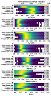 |
Fig. 2. 1D histograms of solar wind properties for five different coronal hole wind characterizations: Zhao et al. (2009) coronal hole (referred to in this and the following figures as Zhao coronal hole), Xu & Borovsky (2015) coronal hole (referred to in this and the following figures as X&B coronal hole), 7-means CH1, 7-means CH2, and a combination of the two 7-means coronal hole wind types, which is referred to as 7-means CH1+CH2. Solar wind properties from top (a) to bottom (g): Proton speed vp, proton density np, proton temperature Tp, magnetic field strength B, proton-proton collisional age log(acol, p − p), O charge-state ratio |

As shown in Zhao & Landi (2014), D’Amicis et al. (2019), Bale et al. (2019), Stansby et al. (2019), D’Amicis et al. (2021), Wang (2024), coronal hole wind observed from small coronal holes, in particular near the solar activity maximum, exhibits a lower proton temperature on average than coronal hole wind from equatorial coronal holes. This property is not reflected in the Xu & Borovsky (2015) coronal hole wind, which does not distinguish between subtypes of coronal hole wind. To define coronal hole wind, Xu & Borovsky (2015) selected unperturbed coronal hole wind from long, repeating high-speed streams. Recurrent coronal hole wind streams like this are observed during the declining phase of the solar activity maximum. This suggests that the initial selection in Xu & Borovsky (2015) is probably biased toward conditions from the declining phase of the solar activity cycle (∼2002) into the solar activity minimum (∼2008) and coronal hole wind from larger coronal holes.
The combination of the two 7-means coronal hole wind types (CH1+CH2) is very similar to the Xu & Borovsky (2015) coronal hole wind in all seven solar wind properties. This suggests that the data-driven 7-means identification of coronal hole wind agrees well with the Xu & Borovsky (2015) scheme. With k = 7, however, k-means identified two subtypes of coronal hole wind, CH1 and CH2. Although both fit the expectations for coronal hole wind, their properties differ systematically from each other. Overall, CH1 remains more similar to the Xu & Borovsky (2015) coronal hole wind, whereas CH2 favors (relatively) higher O and Fe charge states, a younger proton-proton collosional age, a higher magnetic field strength, and a higher proton density. Different subtypes of coronal hole wind were identified in previous studies. For example, Zhao & Landi (2014) investigated the properties of coronal hole wind from polar and equatorial coronal holes separately and found that coronal hole wind from equatorial coronal holes tends to exhibit (slightly) higher O charge states, a younger proton-proton collisional age, and a higher magnetic field strength, which fits the properties of the 7-means CH2 type. This hints at the interpretation that 7-means probably also separated polar from equatorial coronal hole wind. As discussed, for example, by Wang & Ko (2019), equatorial coronal holes usually feature stronger footpoint fields that are probably associated with CH2 here, whereas weaker footpoint fields (usually observed for polar coronal holes) appear to be associated with CH1. Thereby, CH2 probably corresponds to Alfvénic slow solar wind (D’Amicis & Bruno 2015) that originates in small low-latitude coronal holes. CH1 is more likely related to large low-latitude coronal holes that are often extensions of the polar coronal holes and tend to be found near decayed remnants of active regions and are typical sources of recurrent coronal hole wind. This is consistent with the observations by Wang & Ko (2019), D’Amicis et al. (2019, 2021), Bale et al. (2019), Stansby et al. (2019), Wang (2024), who identified similar properties for solar wind from small equatorial coronal holes. Heidrich-Meisner et al. (2016) reported variations in the Fe charge states even within the same coronal hole wind streams. The 7-means classification apparently also relies on this property to characterize its second coronal hole wind type CH2.
With the possible exception of the Zhao et al. (2009) coronal hole wind, Fig. 2 illustrates that all four considered solar wind types indeed exhibit the properties that are expected for coronal hole wind. For the context of this study, we consider this as a validation that these indeed all identify coronal hole wind. In Sect. 4 we investigate the systematic differences between these four coronal hole wind types in more detail.
4. Comparison of coronal hole wind types
The solar wind fractions shown in Fig. 1 already illustrate considerable differences between the coronal hole wind identified by the Zhao et al. (2009) and the Xu & Borovsky (2015) solar wind classifications. The comparison in Neugebauer et al. (2016), who found good agreement between the Zhao et al. (2009) and Xu & Borovsky (2015) coronal hole winds, focused on the time period when the Genesis mission (Lo et al. 2001) was active (late 2001 – early 2004). Fig. 1 shows that during this time period, the coronal hole wind fractions of Zhao et al. (2009) and Xu & Borovsky (2015) are indeed similar. However, the differences are more pronounced during the rest of the solar activity cycle. The most striking difference occurs in 2009, for which the scheme by Zhao et al. (2009) classifies almost all solar wind as coronal hole wind, while the other three coronal hole wind types Xu & Borovsky (2015) coronal hole wind and 7-means CH1 and CH2) observe only very small fractions of coronal hole wind. However, this is not the only interesting feature in Fig. 1. During the complete solar activity minimum period (2006–2009), Zhao et al. (2009) determined a higher fraction of coronal hole wind than the other three coronal hole wind types. This is also visible in Figure 1 of Zhao et al. (2009). During the solar activity maximum, the observed coronal hole wind fractions are more similar (with the exception of CH1). It is interesting to note that from the two 7-means coronal hole wind types, CH1 is dominant during the solar activity minimum, whereas CH2 is more frequent during the solar activity maximum. Therein, during the solar activity minimum period the fraction of CH1 is similar to that of Xu & Borovsky (2015). During the solar activity maximum, however, the CH2 fraction is similar to Xu & Borovsky (2015).
4.1. Effect of changes in the solar wind properties with the solar activity cycle on coronal hole wind classification
Fig. 3 provides an overview of the change in solar wind properties with the solar activity cycle (compare, e.g., Zurbuchen et al. 2002; Zhao et al. 2009; Shearer et al. 2014). For the sake of brevity, we only show four solar wind parameters:  in the top left (panels (a)–(d)),
  in the top right (panels (e)–(h)), vp in the bottom left (panels (i)–(l)), Tp in the bottom right (panels (m)–(p)). In each panel, 1D histograms that each represent three Carrington rotations are shown for the respective solar wind parameter. Each of the four panels includes one panel per coronal hole wind type.
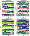 |
Fig. 3. 1D histograms of solar wind properties over time. Each 1D histogram represents three consecutive Carrington rotations. |


The charge states are higher on average during the solar activity maximum (approximately 2002–2004) than during the solar activity minimum (approximately 2006–2009). The effect is stronger for the O charge-state ratio than for the average Fe charge state. This observation holds for each solar wind type shown here individually and also for all solar wind observations. In particular, in 2008–2009 almost all solar wind observations are below the threshold of Zhao et al. (2009). The trend of decreasing  is broken in panel (a) for the Zhao et al. (2009) coronal hole wind. The
  suddenly increases again here. For the other three coronal hole wind types (panels (b)–(d)),
  increases later with the onset of the next solar cycle in 2010. A similar (but less pronounced) effect is visible for
  in panels (e)–(h). Again, the charge states increase for the Zhao et al. (2009) coronal hole wind at least a year earlier than for the other three solar wind types. We expect that the requirement of a minimum number of counts for O and Fe in SWICS results in a selection bias that contributes to the low number of coronal hole wind observations in 2009. This requirement systematically removes some very diluted plasma in all figures, which is most likely to be observed from polar coronal holes during the solar activity minimum.
Panels (i)–(l) show the temporal evolution of vp from 2001–2010. The proton speed is high for all coronal hole wind types and varies from one Carrington rotation to the next. During the solar activity maximum (∼2003), this variability is weakest for CH1, which tentatively implies that pure polar coronal hole wind (from coronal holes with a weak footpoint strength) is rarer during this time period. The variability is strongest for the Zhao et al. (2009) coronal hole wind. Two tracks are visible: one with high solar wind speeds (frequently around 600 km/s), and a second speed with lower proton speeds (around and even below 400 km/s). While proton speeds of about 400 km/s are also observed for the Xu & Borovsky (2015) coronal hole wind and the two 7-means coronal hole wind types (CH1 and CH2), these are considerably more frequent in the Zhao et al. (2009) coronal hole wind. This apparent bifurcation in the proton speeds of the Zhao et al. (2009) coronal hole wind begins approximately in 2005 and lasts until the end of the studied time period. A similar behavior is shown for the proton temperature in panels (m)–(p)). While the Xu & Borovsky (2015) coronal hole wind and 7-means CH1 and CH2 show more consistently high proton temperatures during the complete part of the solar activity cycle shown here, the proton temperatures of the Zhao et al. (2009) coronal hole wind exhibit a similar bifurcation effect as for the proton speeds. From approximately 2005 to the end of 2010, the Zhao et al. (2009) coronal hole wind contains a mixture of cold and hot plasma. In particular, in 2009 (and a few months before), only the cold and slow component remains in the Zhao et al. (2009) coronal hole wind. Xu & Borovsky (2015) coronal hole wind (panel n)) and CH2 (panel p)) share a peak in the average proton temperature at the end of 2005. This might indicate strong wave activity during this time period, but might also be a side-effect of constant thresholds for Xu & Borovsky (2015) and CH2.
These observations suggest the interpretation that the fixed threshold of the scheme by Zhao et al. (2009) misses the underlying changes in the charge-state composition with the solar activity cycle and therefore likely mistakes increasingly more slow solar wind for coronal hole wind during the solar activity minimum. Although all solar wind categorizations considered here rely on fixed thresholds that do not change with the solar activity cycle, the scheme by Zhao et al. (2009) is most affected by this. The two coronal hole wind types identified by 7-means circumvent this problem partially insofar as CH1 represents properties of smaller coronal holes that are dominant during the solar activity maximum, and CH2 represents properties of larger coronal holes that are dominant during the solar activity minimum.
4.2. Changing importance of the solar wind parameters for identifying coronal hole wind
To provide an additional perspective, Fig. 4 shows an explainability measure that quantifies how relevant each solar wind parameter is for an identification as coronal hole wind (high absolute SHAP values > 0). To simplify the representation, we only focused on positive SHAP values. Low absolute values indicate that a solar wind parameter value is not important at this time. In addition, for each solar wind parameter, Fig. 4 differentiates between high feature values (above the median; solid lines) and low feature values (below the median; dashed lines), as introduced in Sect. 2.2.
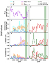 |
Fig. 4. Averaged SHAP values per three Carrington rotations over time for solar wind parameter and coronal hole wind type. From top to bottom: Zhao et al. (2009) coronal hole, Xu & Borovsky (2015) coronal hole, 7-means CH1, and 7-means CH2. Green shading highlights 2009. The SHAP values for seven considered solar wind parameters are distributed in the left and right columns. The left column shows np, Tp, B, and |


Panels (a) and (b) plots the respective SHAP values averaged over three Carrington rotations for the Zhao et al. (2009) coronal hole wind. As expected, the O charge-state ratio is the only parameter that is relevant for identifying coronal hole wind. The six curves for the six other parameters are included, but are all plotted on top of each other at the zero line in the left and right panels. In the right panel, a small peak for the proton speed is just visible in 2002. That the SHAP values indeed correctly identify that the parameters that are by design not relevant for identifying coronal hole wind in the Zhao et al. (2009) scheme are unimportant (i.e., have low absolute SHAP values close to zero) provides a basic sanity check for the interpretation of SHAP values. Low O charge-state ratios (dashed lines in Fig. 4) are relevant for recognizing solar wind as Zhao et al. (2009) coronal hole wind. Since Fig. 4 only shows positive values, the respective high importance of high O charge-state ratios for identifying noncoronal hole wind is not directly visible. We omitted negative SHAP values to simplify the representation and focus only on the coronal hole types. However, in particular during 2008–2009, the importance of the O charge-state ratio for the Zhao et al. (2009) scheme is reduced, and the solid line becomes visible for several Carrington rotations. This can be understood as a consequence of the following effect: During this time period, (almost) all solar wind observations have  below the decision threshold, as shown in Fig. 3. In addition, the median of all considered
  observations is with 0.095 below the Zhao et al. (2009) threshold for identifying coronal hole wind. Thus, the two curves merge when (almost) no observations above the Zhao et al. (2009) threshold are observed during a Carrington rotation. Further, the actual value of
  no longer plays a role (and receives a lower absolute value in its SHAP value) since the classification is (almost) always the same here.
Panels (c) and (d) shows the corresponding SHAP values for Xu & Borovsky (2015) coronal hole wind. Most of the time, high proton temperatures, low proton densities, and high proton speeds are relevant for identifying coronal hole wind. Although the scheme by Xu & Borovsky (2015) also depends on the magnetic field strength, B is less relevant for distinguishing coronal hole wind from noncoronal hole wind. For the classification by Xu & Borovsky (2015), two time periods stand out with very low SHAP values: around the middle of 2004 and 2009. For these time periods, Fig. 1 showed very low fractions of Xu & Borovsky (2015) coronal hole wind. Thus, the precise values of the solar wind parameters are not important during these times for identifying Xu & Borovsky (2015) coronal hole wind, since (almost) all observations here are noncoronal hole wind. According to Xu & Borovsky (2015), coronal hole wind was characterized based on unperturbed coronal hole wind from repeating high-speed streams. Since repeating high-speed streams are more likely to be observed during the solar activity minimum, this characterization probably introduced a selection bias toward coronal hole wind from polar (or larger equatorial) coronal holes with a low footpoint field strength and a corresponding bias against coronal hole wind from smaller equatorial coronal holes with a higher footpoint field strength. This bias probably reduces the fraction of Xu & Borovsky (2015) coronal hole wind in 2004, but not in 2009.
Panels (e)–(h) provide an overview of the importance of each considered solar wind parameter for 7-means CH1 and 7-means CH2. All seven solar wind parameters play some role in identifying these two solar wind types. Overall, for 7-means CH1, low values of the O charge-state ratio and the average Fe charge state (dashed purple and dark green lines in panels (e) and (f)) and high values of the proton speed and proton temperature (red and orange solid lines panels (e) and (f)) are the most important (single) parameters for 7-means CH1. For 7-means CH2, the average high values of the average Fe charge state (solid dark green lines in panel h), high values of the proton speed and proton temperature (solid red and orange lines in panels (g) and (h)) are most important. In agreement with Fig. 1, the importance of most solar wind parameters for identifying 7-means CH1 is higher during the solar activity minimum (in particular, in 2006–2008) and low during the solar activity maximum (in particular, in 2003–2004), whereas the opposite is the case for 7-means CH2.
In 2009 the SHAP values for all four coronal hole wind types and all parameters are low because (almost) all solar wind (as was the case for Zhao et al. 2009) is seen as coronal hole wind, or (almost) no solar wind is identified as coronal hole wind (as was the case for the other three coronal hole wind types).
4.3. Low fraction of coronal hole wind in 2009
Fujiki et al. (2016) investigated the size of the coronal hole area over several solar cycles. In particular, Figures 3 and 4 in Fujiki et al. (2016) show almost no coronal holes at low latitudes (below 30° latitude) in 2009. A similar effect is visible in Figure 3 in Fujiki et al. (2016) at the ends of the previous solar cycles. In 2003, when Xu & Borovsky (2015) sees a high fraction of coronal hole wind, Figure 4 in Fujiki et al. (2016) shows an unusually large area of equatorial coronal holes. Thus, ACE probably was connected more frequently to equatorial coronal holes in 2003 and therefore observed a high fraction of coronal hole wind. Since ACE is located close to the ecliptic, ACE tends to be more frequently connected to low-latitude coronal holes than to high-latitude coronal holes (in particular, under stable solar activity minimum conditions). This supports the low fraction of coronal hole wind in 2009 determined by Xu & Borovsky (2015) and 7-means. The small fraction of remaining coronal hole wind appears to originate at higher latitudes.
5. Conclusion
Coronal hole wind is considered the best-understood component of the solar wind (Marsch 2006; Cranmer 2009) and different solar wind categorizations have been reported to agree well in their respective coronal hole wind identification (Neugebauer et al. 2016). However, coronal hole wind is not uniform in its properties. Differences between equatorial and polar coronal hole wind were identified, for example, by Zhao & Landi (2014) and Wang (2016), and the O-cool coronal hole wind can be Fe-hot or Fe-cool (Heidrich-Meisner et al. 2016). Nevertheless, established solar wind categorizations that rely on fixed decision boundaries (e.g., Zhao et al. 2009; Xu & Borovsky 2015) differ in where exactly these decision boundaries should separate coronal hole wind from slow solar wind. This study was motivated by the drastically different coronal hole wind fractions observed by Zhao et al. (2009) and Xu & Borovsky (2015) during the solar activity minimum. As an alternative, purely data-driven perspectives of coronal hole wind identified by an unsupervised machine-learning method k-means (here, with k = 7) was included in the comparison. Therein, 7-means identifies two types of coronal hole wind, here called CH1 and CH2. Both exhibit typical properties of coronal hole wind, but while CH1 (based on the properties of polar and equatorial or weak and strong footpoint-field coronal hole wind reported in Zhao & Landi 2014; Wang 2016; Wang & Ko 2019) appears to favor polar coronal hole wind with weak footpoint fields, CH2 appears to mainly include equatorial coronal hole wind with high average Fe charge state and high footpoint strengths.
We identified the reliance on fixed thresholds as the main cause for the disparity in the determined coronal hole fractions of Zhao et al. (2009) compared to the other three coronal hole wind types: The O charge-state ratio  is known to vary systematically with the solar activity cycle (Zurbuchen et al. 2002; Zhao et al. 2009; Shearer et al. 2014). The fixed threshold by Zhao et al. (2009) appears to be best adjusted to solar activity maximum conditions when the agreement with Xu & Borovsky (2015) is high, as discussed in Neugebauer et al. (2016), but appears less appropriate for the solar activity minimum. For the scheme by Zhao et al. (2009), this evidently leads to a misclassification of slow solar wind as coronal hole wind during the solar activity minimum. The Xu & Borovsky (2015) coronal hole wind appears to be better adjusted to solar activity minimum than solar activity maximum conditions.
The very low fraction of coronal hole wind identified in 2009 by Xu & Borovsky (2015) and 7-means could also be a result of their respective fixed decision boundaries since these methods are also adversely affected by ignoring the systematic changes in the solar wind with the solar activity cycle. However, this low fraction of coronal hole wind observed at L1 by ACE in 2009 is probably also related to the very small number of coronal holes at low latitudes in 2009 (Fujiki et al. 2016).
We conclude that the solar wind categorization needs to be revisited even to identify coronal hole wind. An improved solar wind categorization should take the phase of the solar cycle explicitly into account. Further, an optimal set of input parameters for solar wind classification should be refined and should include a more direct measure of wave activity, for example, the Alfvénicity parameter Ko et al. (2018), Wang & Ko (2019).
In this context, “winning” or “loosing” is not associated with any preference for which result would be better.
Acknowledgments
This work was supported by the Deutsches Zentrum für Luft- und Raumfahrt (DLR) as SOHO/CELIAS 50 OC 2104. We further thank the science teams of ACE/SWEPAM, ACE/MAG as well as ACE/SWICS for providing the respective level 2 and level 1 data products.
References
- Alelyani, S., Tang, J., & Liu, H. 2018, Data Clustering, 29 [Google Scholar]
- Amaya, J., Dupuis, R., Innocenti, M. E., & Lapenta, G. 2020, FrASS, 7, 66 [NASA ADS] [Google Scholar]
- Bale, S. D., Badman, S. T., Bonnell, J. W., et al. 2019, Nature, 576, 237 [NASA ADS] [CrossRef] [Google Scholar]
- Bale, S. D., Drake, J. F., McManus, M. D., et al. 2023, Nature, 618, 252 [NASA ADS] [CrossRef] [Google Scholar]
- Berger, L. 2008, Ph.D. Thesis, Kiel, Christian-Albrechts-Universität [Google Scholar]
- Berger, L., Wimmer-Schweingruber, R. F., & Gloeckler, G. 2011, Phys. Rev. Lett., 106, 151103 [NASA ADS] [CrossRef] [Google Scholar]
- Berger, L., Heidrich-Meisner, V., Teichmann, S., & Wimmer-Schweingruber, R. F. 2023, Solar Wind properties measured with instruments on the Advanced Composition Explorer (ACE) [Google Scholar]
- Bloch, T., Watt, C., Owens, M., McInnes, L., & Macneil, A. R. 2020, Sol. Phys., 295, 41 [NASA ADS] [CrossRef] [Google Scholar]
- Camporeale, E., Carè, A., & Borovsky, J. E. 2017, J. Geophys. Res., 122, 910 [NASA ADS] [CrossRef] [Google Scholar]
- Cane, H. V., & Richardson, I. G. 2003, J. Geophys. Res., 108, 1156 [Google Scholar]
- Chitta, L. P., Zhukov, A. N., Berghmans, D., et al. 2023, Science, 381, 867 [NASA ADS] [CrossRef] [Google Scholar]
- Cranmer, S. R. 2009, LRSP, 6, 3 [NASA ADS] [Google Scholar]
- D’Amicis, R., & Bruno, R. 2015, ApJ, 805, 84 [Google Scholar]
- D’Amicis, R., Matteini, L., & Bruno, R. 2019, MNRAS, 483, 4665 [NASA ADS] [Google Scholar]
- D’Amicis, R., Perrone, D., Bruno, R., & Velli, M. 2021, J. Geophys. Res., 126, e28996 [Google Scholar]
- Elliott, H. A., McComas, D. J., Schwadron, N. A., et al. 2005, J. Geophys. Res., 110, A04103 [NASA ADS] [Google Scholar]
- Fujiki, K., Tokumaru, M., Hayashi, K., Satonaka, D., & Hakamada, K. 2016, ApJ, 827, L41 [NASA ADS] [CrossRef] [Google Scholar]
- Gloeckler, G., Cain, J., Ipavich, F. M., et al. 1998, Space Sci. Rev., 86, 497 [NASA ADS] [CrossRef] [Google Scholar]
- Heidrich-Meisner, V., & Wimmer-Schweingruber, R. F. 2018, Machine learning techniques for space weather (Elsevier), 397 [CrossRef] [Google Scholar]
- Heidrich-Meisner, V., Peleikis, T., Kruse, M., Berger, L., & Wimmer-Schweingruber, R. 2016, A&A, 593, A70 [NASA ADS] [CrossRef] [EDP Sciences] [Google Scholar]
- Heidrich-Meisner, V., Berger, L., & Wimmer-Schweingruber, R. F. 2020, A&A, 636, A103 [NASA ADS] [CrossRef] [EDP Sciences] [Google Scholar]
- Huang, J., Kasper, J. C., Vech, D., et al. 2020, ApJS, 246, 70 [Google Scholar]
- Hundhausen, A. J., Gilbert, H. E., & Bame, S. J. 1968, ApJ, 152, L3 [Google Scholar]
- Jian, L., Russell, C. T., Luhmann, J. G., & Skoug, R. M. 2006, Sol. Phys., 239, 393 [NASA ADS] [CrossRef] [Google Scholar]
- Jian, L. K., Russell, C. T., & Luhmann, J. G. 2011, Sol. Phys., 274, 321 [Google Scholar]
- Kasper, J. C., Lazarus, A. J., Gary, S. P., & Szabo, A. 2003, in Solar Wind Ten, eds. M. Velli, R. Bruno, F. Malara, & B. Bucci (AIP), AmJPh, 679, 538 [NASA ADS] [CrossRef] [Google Scholar]
- Kasper, J. C., Stevens, M. L., Korreck, K. E., et al. 2012, ApJ, 745, 162 [Google Scholar]
- Ko, Y.-K., Roberts, D. A., & Lepri, S. T. 2018, ApJ, 864, 139 [NASA ADS] [CrossRef] [Google Scholar]
- Krieger, A. S., Timothy, A. F., & Roelof, E. C. 1973, Sol. Phys., 29, 505 [NASA ADS] [CrossRef] [Google Scholar]
- Kumar, V., & Minz, S. 2014, SmartCR, 4, 211 [Google Scholar]
- Lloyd, S. 1982, ITIT, 28, 129 [Google Scholar]
- Lo, M. W., Williams, B. G., Bollman, W. E., et al. 2001, AdAns, 49, 169 [Google Scholar]
- Lundberg, S. M., & Lee, S. I. 2017, NIPS, 30 [Google Scholar]
- Marsch, E. 2006, LRSP, 3, 1 [NASA ADS] [Google Scholar]
- Marsch, E., Rosenbauer, H., Schwenn, R., Muehlhaeuser, K. H., & Denskat, K. U. 1981, J. Geophys. Res., 86, 9199 [NASA ADS] [CrossRef] [Google Scholar]
- Marsch, E., Goertz, C. K., & Richter, K. 1982a, J. Geophys. Res., 87, 5030 [NASA ADS] [CrossRef] [Google Scholar]
- Marsch, E., Schwenn, R., Rosenbauer, H., et al. 1982b, J. Geophys. Res., 87, 52 [Google Scholar]
- Marsch, E., Zhao, L., & Tu, C. Y. 2006, AnGeo, 24, 2057 [Google Scholar]
- McComas, D. J., Bame, S. J., Barker, P. L., et al. 1998, Geophys. Res. Lett., 25, 4289 [NASA ADS] [CrossRef] [Google Scholar]
- Neugebauer, M., Reisenfeld, D., & Richardson, I. G. 2016, J. Geophys. Res., 121, 8215 [NASA ADS] [CrossRef] [Google Scholar]
- Parker, E. N. 1965, Space Sci. Rev., 4, 666 [Google Scholar]
- Richardson, I. G., & Cane, H. V. 2010, Sol. Phys., 264, 189 [NASA ADS] [CrossRef] [Google Scholar]
- Shapley, L. S. 1953, A value for n-person games (Princeton: Princeton University Press) [Google Scholar]
- Shearer, P., von Steiger, R., Raines, J. M., et al. 2014, ApJ, 789, 60 [NASA ADS] [CrossRef] [Google Scholar]
- Smith, C. W., L’Heureux, J., Ness, N. F., et al. 1998, Space Sci. Rev., 86, 613 [Google Scholar]
- Solorio-Fernández, S., Carrasco-Ochoa, J. A., & Martínez-Trinidad, J. F. 2020, Artif. Intell. Rev., 53, 907 [CrossRef] [Google Scholar]
- Stansby, D., Horbury, T. S., & Matteini, L. 2019, MNRAS, 482, 1706 [Google Scholar]
- Teichmann, S., Heidrich-Meisner, V., Berger, L., & Wimmer-Schweingruber, R. 2023, Feature selection with k-means on solar wind data [Google Scholar]
- Tu, C.-Y., Zhou, C., Marsch, E., et al. 2005, Science, 308, 519 [Google Scholar]
- Verscharen, D., Klein, K. G., & Maruca, B. A. 2019, LRSP, 16, 5 [NASA ADS] [Google Scholar]
- Vidotto, A. A. 2021, LRSP, 18, 3 [NASA ADS] [Google Scholar]
- Wang, Y. M. 2016, ApJ, 833, L21 [NASA ADS] [CrossRef] [Google Scholar]
- Wang, Y. M. 2024, Sol. Phys., 299, 54 [NASA ADS] [CrossRef] [Google Scholar]
- Wang, Y. M., & Ko, Y. K. 2019, ApJ, 880, 146 [NASA ADS] [CrossRef] [Google Scholar]
- Xu, F., & Borovsky, J. E. 2015, J. Geophys. Res., 120, 70 [NASA ADS] [CrossRef] [Google Scholar]
- Zhao, L., & Landi, E. 2014, ApJ, 781, 110 [NASA ADS] [CrossRef] [Google Scholar]
- Zhao, L., Zurbuchen, T. H., & Fisk, L. A. 2009, Geophys. Res. Lett., 36, L14104 [NASA ADS] [CrossRef] [Google Scholar]
- Zurbuchen, T. H., Fisk, L. A., Gloeckler, G., & von Steiger, R. 2002, Geophys. Res. Lett., 29, 1352 [Google Scholar]
All Figures
|
Fig. 1. Fractions of solar wind types from three solar wind classifications per three Carrington rotations. From left to right: (a) Zhao et al. (2009), (b) Xu & Borovsky (2015), and (c) 7-means clustering. The green shading highlights 2009. All noncoronal hole wind types (Panel a): Slow and ICME. Panel (b): Sector-reversal, helmet streamer, and ejecta. Panel (c): Remaining five types identified by 7-means (numbered as types T1, ..., T5) are shown in different shades of gray to keep the focus on the coronal hole wind types of interest. |
| In the text | |
|
Fig. 2. 1D histograms of solar wind properties for five different coronal hole wind characterizations: Zhao et al. (2009) coronal hole (referred to in this and the following figures as Zhao coronal hole), Xu & Borovsky (2015) coronal hole (referred to in this and the following figures as X&B coronal hole), 7-means CH1, 7-means CH2, and a combination of the two 7-means coronal hole wind types, which is referred to as 7-means CH1+CH2. Solar wind properties from top (a) to bottom (g): Proton speed vp, proton density np, proton temperature Tp, magnetic field strength B, proton-proton collisional age log(acol, p − p), O charge-state ratio |
| In the text | |
|
Fig. 3. 1D histograms of solar wind properties over time. Each 1D histogram represents three consecutive Carrington rotations. |
| In the text | |
|
Fig. 4. Averaged SHAP values per three Carrington rotations over time for solar wind parameter and coronal hole wind type. From top to bottom: Zhao et al. (2009) coronal hole, Xu & Borovsky (2015) coronal hole, 7-means CH1, and 7-means CH2. Green shading highlights 2009. The SHAP values for seven considered solar wind parameters are distributed in the left and right columns. The left column shows np, Tp, B, and |
| In the text | |
Current usage metrics show cumulative count of Article Views (full-text article views including HTML views, PDF and ePub downloads, according to the available data) and Abstracts Views on Vision4Press platform.
Data correspond to usage on the plateform after 2015. The current usage metrics is available 48-96 hours after online publication and is updated daily on week days.
Initial download of the metrics may take a while.