| Issue |
A&A
Volume 635, March 2020
|
|
|---|---|---|
| Article Number | A17 | |
| Number of page(s) | 11 | |
| Section | Interstellar and circumstellar matter | |
| DOI | https://doi.org/10.1051/0004-6361/201936725 | |
| Published online | 02 March 2020 | |
Seeds of Life in Space (SOLIS)
V. Methanol and acetaldehyde in the protostellar jet-driven shocks L1157-B0 and B1
1
INAF, Osservatorio Astrofisico di Arcetri,
Largo E. Fermi 5,
50125
Firenze, Italy
e-mail: codella@arcetri.astro.it
2
Univ. Grenoble Alpes, CNRS, Institut de Planétologie et d’Astrophysique de Grenoble (IPAG),
38000
Grenoble,
France
3
Dipartimento di Chimica, Biologia e Biotecnologie,
Via Elce di Sotto 8,
06123
Perugia, Italy
4
Max-Planck-Institut für extraterrestrische Physik (MPE),
Giessenbachstrasse 1,
85748
Garching, Germany
5
National Astronomical Observatory of China,
Datun Road 20,
Chaoyang,
Beijing
100012, PR China
6
CAS Key Laboratory of FAST, NAOC, Chinese Academy of Sciences,
Chaoyang, PR China
7
National Astronomical Observatory of Japan,
2 Chome-21-1 Osawa,
Mitaka-shi,
Tokyo-to
181-0015, Japan
8
Institut de Radioastronomie Millimétrique, 300 rue de la Piscine, Domaine Universitaire de Grenoble,
38406
Saint-Martin d’Hères,
France
Received:
18
September
2019
Accepted:
23
December
2019
Context. It is nowadays clear that a rich organic chemistry takes place in protostellar regions. However, the processes responsible for it, that is, the dominant formation routes to interstellar complex organic molecules, are still a source of debate. Two paradigms have been evoked: the formation of these molecules on interstellar dust mantles and their formation in the gas phase from simpler species previously synthesised on the dust mantles.
Aims. In the past, observations of protostellar shocks have been used to set constraints on the formation route of formamide (NH2CHO), exploiting its observed spatial distribution and comparison with astrochemical model predictions. In this work, we follow the same strategy to study the case of acetaldehyde (CH3CHO).
Methods. To this end, we used the data obtained with the IRAM-NOEMA interferometer in the framework of the Large Program SOLIS to image the B0 and B1 shocks along the L1157 blueshifted outflow in methanol (CH3OH) and acetaldehyde line emission.
Results. We imaged six CH3OH and eight CH3CHO lines which cover upper-level energies up to ~30 K. Both species trace the B0 molecular cavity as well as the northern B1 portion, that is, the regions where the youngest shocks (~1000 yr) occurred. The CH3OH and CH3CHO emission peaks towards the B1b clump, where we measured the following column densities and relative abundances: 1.3 × 1016 cm−2 and 6.5 × 10⁻⁶ (methanol), and 7 × 1013 cm−2 and 3.5 × 10⁻⁸ (acetaldehyde). We carried out a non-LTE (non-Local Thermodinamic Equilibrium) Large Velocity Gradient (LVG) analysis of the observed CH3OH line: the average kinetic temperature and density of the emitting gas are Tkin ~ 90 K and nH2 ~ 4 × 105 cm−3, respectively. The CH3OH and CH3CHO abundance ratio towards B1b is 190, varying by less than a factor three throughout the whole B0–B1 structure.
Conclusions. Comparison of astrochemical model predictions with the observed methanol and acetaldehyde spatial distribution does not allow us to distinguish whether acetaldehyde is formed on the grain mantles or in the gas phase, as its gas-phase formation, which is dominated by the reaction of ethyl radical (CH3CH2) with atomic oxygen, is very fast. Observations of acetaldehyde in younger shocks, for example those of ~102 yr old, and/or of the ethyl radical, whose frequencies are not presently available, are necessary to settle the issue.
Key words: stars: formation / ISM: jets and outflows / ISM: molecules / ISM: individual objects: L1157
© ESO 2020
1 Introduction
One of the open questions in astrochemistry refers to how chemistry richness develops and evolves in star forming regions. More specifically, the molecular complexity during the evolutionary stages that lead a molecular cloud to form a solar-type star and its planetary system has yet to be elucidated. Particularly relevant are the abundances of the so-called interstellar complex organic molecules (iCOMs: molecules with at least six atoms: Herbst & van Dishoeck 2009; Ceccarelli et al. 2017), as they may be considered as small blocks from which complex pre-biotic species can build up (e.g. Caselli & Ceccarelli 2012; Belloche et al. 2014). The present consensus is that after an initial cold phase in which icy mantles enriched with hydrogenated species formon the dust grains (e.g. Tielens & Hagen 1982; Watanabe & Kouchi 2002; Rimola et al. 2014), the iCOMs synthesis can either occur on the grain mantle surfaces initiated by energetic processing (e.g. Garrod & Herbst 2006; Garrod et al. 2008; Ruaud et al. 2015; Vasyunin et al. 2017) or in the gas phase initiated by the sublimation of the mantles themselves (e.g. Charnley et al. 1992; Balucani et al. 2015; Codella et al. 2017; Skouteris et al. 2018). In both cases, the composition of the grain mantles therefore plays a paramount role in the gaseous, observable abundance of iCOMs (see e.g. Burkhardt et al. 2019) – in the former possible scenario, because the mantle species are directly injected from the mantles into the gas; and in the latter possible scenario, because they feed gas reactions leading to iCOMs.
In this context, protostellar shocks are particularly precious because they can provide not only the observed iCOM abundances but also the approximate times at which they are formed. Indeed, at the passage of the shock, molecules present in the grain mantles are injected into the gas phase either because of sputtering (gas–grain collisions) or shattering (grain–grain) processes (e.g. Flower & Pineau des Forêts 1994; Caselli et al. 1997; Schilke et al. 1997; Gusdorf et al. 2008a,b). Once in the gas phase, the injected mantle species undergo reactions that destroy and/or form iCOMs (unless multiple shocks occur at the very same place, which is unlikely): therefore, the gaseous iCOM abundances are intrinsically time dependent. Fortunately, the chemical evolution time, which is a few thousand years at most, is of the order of the age of young protostellar shocks (e.g. Herbst & van Dishoeck 2009; Ceccarelli et al. 2017). Thus, sufficiently high spatial resolution observations towards these objects allow us to decipher the different time-dependent abundances of iCOMs and consequently provide extremely strong constraints on the formation and destruction of iCOMs. For example, this method was applied to constrain the formation route of formamide in the jet-driven protostellar shock L1157-B1 (Codella et al. 2017; hereinafter CC17). Previous observations have shown that this latter shock is extremely rich in iCOMs (Arce et al. 2008; Lefloch et al. 2017), suggesting that it may be an ideal case to look for others with the same method as that used by Codella et al. (2017)
In this article, we continue the systematic study of the formation and destruction routes for iCOMs in the L1157-B1 shock started in CC17. Here we focus on the acetaldehyde (CH3 CHO) and methanol (CH3OH). As in CC17, we make use of the observations from the IRAM/NOEMA (NOrthern Extended Millimeter Array1) Large Project SOLIS (Seeds Of Life In Space; Ceccarelli et al. 2017), whose goal is to investigate the formation and destruction of iCOMs during the early stages of solar-type star formation. The article is organised as follows: in Sect. 2 we describe the source and summarise the previous studies of its astrochemistry. In Sect. 3 we describe the observations, in Sect. 4 we report the results of the analysis of these observations, in Sect. 5 we discuss the impact of those results, and in Sect. 6 we present our conclusions.
2 L1157-B1: an astrochemical laboratory
The chemically rich molecular outflow driven by the L1157-mm Class 0 protostar (d = 352 pc; Zucker et al. 2019) has been extensively used to investigate how the gas chemistry is altered by the injection of the species frozen onto the dust mantles. L1157-mm drives an episodic and precessing jet (Gueth et al. 1996; Podio et al. 2016), which produced several cavities well observed using both single-dish antennas and interferometers (e.g. Gueth et al. 1998; Lefloch et al. 2012). In particular, the southern blueshifted outflow is associated with several shocked regions produced by impacts between jets and cavities called B0, B1, and B2 (see also Fig. 1). The brightest shocked region, B1, is one of the targets of the IRAM NOEMA SOLIS Large Program. In particular, B1 consists of aseries of shocks caused by different episodes of ejection hitting the cavity wall. These shocks produced a clumpy structure (identified using several molecular species, see e.g. Tafalla & Bachiller 1995; Codella et al. 2009; Lefloch et al. 2012; Benedettini et al. 2013), which can be classified as follows: (i) a northern arch-like structure composed of the clumps B1a-e-f-b (see Fig. 1), plus (ii) two clumps, labelled B1c and B1d, which are the oldest ones (kinematical age ~ 1400 yr, from Podio et al. 2016, corrected for the new distance of 352 pc by Zucker et al. 2019), being the farthest away from the source, closeto the B1 apex.
Within the context of the study of iCOMs, the advantages of observing L1157-B1 are that: (i) the observations are not polluted by the protostar emission, as it is located at a projected distance of 0.11 pc, and (ii) several previous studies have shown that grain-mantle species have been injected, due to shock-induced sputtering and shattering, into the gas phase (e.g. Bachiller et al. 2001; Arce et al. 2008; Codella et al. 2010; Fontani et al. 2014; Lefloch et al. 2017).
In the first SOLIS paper on L1157-B1 (CC17), we compared the spatial distribution of the acetaldehyde (CH3 CHO) line emission with that from formamide (NH2CHO), finding a striking chemical stratification. This implies a NH2 CHO/CH3COH abundance ratio which varies within the B1 structure: specifically, the formamide line emission is associated with older shocked gas with respect to acetaldehyde. Thanks to the comparison of the observations with astrochemical model predictions, we provided evidence that formamide is formed in L1157-B1 by gas-phase chemical reactions. However, we were unable to provide any indication on the formation route of acetaldehyde.
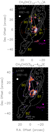 |
Fig. 1 L1157 southern blueshifted lobe in CO (1–0) (white contours; Gueth et al. 1996). The precessing jet ejected by the central object L1157-mm (outside the frame and toward the northwest) excavated several clumpy cavities, named B0, B1, and B2, respectively. The maps are centred at α(J2000) = 20h39m10s.2, δ(J2000) = + 68°01′10′′.5 (Δα = +25′′ and Δδ = −63′′.5 from the L1157-mm protostar). Top panel: map (in colour scale) of the emission due to the CH3 OH(21,2–11,1) A transition (integrated over the whole velocity range). The first contour and step are 3σ (32 mJy beam−1 km s−1). For the CO image, the first contour and step are 6σ (1σ = 0.5 Jy beam−1 km s−1) and 4σ, respectively. The dashed circle shows the primary beam of the CH3OH image (64′′). Yellow labels are for the B0 and B1 clumps (black triangles) previously identified using molecular tracers (see text, and e.g. Benedettini et al. 2007; Codella et al. 2009, 2017). The white and magenta ellipses depict the synthesised beams of the CO (3′′.65×2′′.96, PA = +88°), and CH3 OH (2′′.97×2′′.26, PA = –155°) observations, respectively. Bottom panel: same as top panel but for CH3CHO (50,4 –40,4) E. The first contour and step are 3σ (7 mJy beam−1 km s−1). The synthesised beams of the CH3CHO image are similar to those of the CH3OH map. |
3 Observations
The L1157-B0/B1 shocks were observed at 3 mm with the IRAM NOEMA array during two tracks in October 2016 (7 antennas), and three tracks in January 2017 (8 antennas) using both the C and D configurations. The shortest and longest baselines are 24 and 304 m, respectively. These configurations allowed us to recover emission at scales (with a full efficiency) up to ~ 14′′. The primarybeam was 64′′. The phase centre is α(J2000) = 20h 39m10s.2, δ(J 2000) = +68°01′10′′.5. The CH3OH and CH3CHO lines listed in Table 1 were observed using the WideX backends, with a total spectral band of ~ 4 GHz, and a spectral resolution of1.95 MHz (~6 km s−1). Several CH3OH lines were also observed with 80 MHz backends with a spectral resolution of 156 kHz (~ 0.48 km s−1). Calibration was carried out following standard procedures using GILDAS-CLIC2. The bandpass was calibrated on 3C454.3, while the absolute flux was fixed by observing MWC349, 2200+420, 2013+370, and 2007+659, the latter also being used to set the gains in phase and amplitude. The final uncertainty on the absolute flux scale is ≤ 15%. The phase rms was ≤ 50°, the typical precipitable water vapour (PWV) was from 2 to 20 mm, and the system temperatures were ~ 50–100 K (D) and ~ 50–250 K (C). The rms noise in the 1.95 MHz channels was 4–20 mJy beam−1, depending on the frequency (see Table 1). Images were produced using natural weighting, and restored with a clean beam of 2′′.97 × 2′′.26 (PA = –155°).
4 Results
We imaged six methanol emission lines towards the L1157 blueshifted outflow, covering upper level excitations (Eu) from 7 to 28 K (see Table 1). Figure 1 (top) shows, as an example, the imaging of the CH3OH(21,2–11,1) A line emission on top of the CO (1–0) image (Gueth et al. 1996), which accurately outlines the B0, B1, and B2 cavities opened by the precessing jet driven by L1157-mm, which is located at Δα = –25′′ and Δδ = +63′′.5 with respect to the centre of Fig. 1 map. Figure A.1 shows the images of the whole of the CH3OH line emission reported in Table 1. In addition, we detected and imaged eight acetaldehyde lines (Eu = 14–23 K), which are also reported in Table 1. Figure 1 (bottom) shows the CH3CHO(50,4–40,4) E map, while Fig. A.2 is for all the other CH3CHO images.
Using the ASAI (Astrochemical Surveys At IRAM3; Lefloch et al. 2017, 2018) unbiased spectral survey obtained with the IRAM 30 m antenna, we evaluated the missing flux of the present NOEMA dataset. Comparison between the ASAI and NOEMA spectra indicates that a large fraction (about 60%) of the CH3OH and CH3CHO emission is filtered out, indicating that their emission is extended across structures larger than ~14′′. Indeed, this matches the goal of the present project, which is the analysis of the chemical content of the small structures associated with multiple shocked regions, and without any contribution due to more extended emission. In Sects. 4.3 and 5.1 the present results will be compared with those derived by the analysis based on single-dish observations, showing there is no bias introduced by the missing flux.
4.1 CH3OH and CH3CHO spatial distribution
The present NOEMA CH3OH data improve the images and spectra based on IRAM-PdBI observations of the methanol spectral pattern at 97.94 GHz performed in 1997 using five antennas, and with a synthesised beam of ~ 5′′, as well as those of the 21,1 –11,0 A line, with a spectral resolution of 0.5 km s−1 (Benedettini et al. 2007). The eight CH3CHO images also allow us to perform a deeper analysis with respect to the spatial distributions obtained by Codella et al. (2015), who stacked the CH3CHO (70,7–60,6) E and A lines with an angular resolution of ~ 2′′.5.
The present results are consistent with the previous observations that show that the CH3OH and CH3CHO spatial distributions are in good agreement; both trace the B0 eastern molecular cavity as well as the northern arch-like structure containing B1a-e-f-b. In particular, the peak emission of both species is clearly associated with the B1b clump. In other words, although emission is observed also towards B1c, the bulk of the CH3OH and CH3CHO emission does not come from the southern B1 apex (Codella et al. 2017). Instead, they preferentially trace the region associated with the youngest B1 shock occurring next to the B1a position, where HDCO, a selective tracer of dust mantle release, has been observed (Fontani et al. 2014), as well as high-velocity SiO emission (Gueth et al. 1998; Podio et al. 2016), locating the likely current sputtering of the dust refractory cores due to the shock. These findings are not surprising for methanol, which is efficiently produced on the grain surfaces by CO hydrogenation. On the other hand, they indicate that acetaldehyde is either formed on the mantles as well or that it is quickly (in less than ~ 1000 yr) produced in the gas phase using simpler mantle products (as suggested by Codella et al. 2015). This topic is further discussed in Sect. 5.2.
4.2 Line spectra
Figure 2 shows the spectra extracted from the CH3OH and CH3CHO emission peaks at the B1b position. In addition to methanol and acetaldehyde, in B1b we observe emission at 99.3 GHz due to another iCOM, dimethyl ether (CH3OCH3). In particular, the detected line is due to the 41,4 –30,3 transitions of the EA, AE, EE, and AA isomers, blended at the ~ 2 MHz spectral resolution (see Fig. 2). Finally, we detect several S-bearing species (CS, SO, and OCS isotopologues), which will be analysed in a forthcoming paper on sulphur chemistry (Feng et al., in prep.).
For each detected line, in addition to the spectroscopic parameters, Table 1 reports the intensity integrated over the whole velocity emission range (down to velocities blueshifted by 15 km s−1). The 2 MHz spectral resolution of the WideX backend does not allow us to investigate the iCOMs kinematics. However, we can confirm that all the spectra are blueshifted, in agreement with all the molecular lines so far observed towards L1157-B1 (e.g. Bachiller et al. 2001; Lefloch et al. 2017). In addition, the CH3OH spectral pattern at 96.7 GHz (see Table 1) has been observed with a 0.48 MHz (0.16 km s−1) spectral resolution. Figure 3 reports the spectra as observed towards the B0e and B1b clumps: four transitions of the 2k,k –1k,k pattern are reported, with the corresponding frequencies marked by small vertical red lines. The spectra are centred at 96 741.38 MHz, which is the frequency of the 20,2 –10,1 A line. The methanol lines extracted from the B0e position have a peak velocity of ~ +0.5 km s−1 (VLSR = +2.6 km s−1), and are about 3–4 km s−1 in width (FWHM), with evidence of bluer wings. The B1b spectrum is definitely more complex showing in addition a secondary peak at about –4 km s−1. This high-velocity peak was tentatively detected by Benedettini et al. (2013) using the CH3OH(3k,k–2k,k) emission at 2 mm. In the present dataset, a clear Gaussian-like secondary peak is emerging, definitely offset in velocity from the mean peak. These findings confirm that the northern part of the B1 structure is associated with young shocked gas, here traced by methanol molecules injected into the gas phase at high velocities.
Figure 4 shows the spectral fit of the 2-1,2–1-1,1 E, 20,2 –10,1 A, and 20,2 –10,1 E triplets as observed towards B1b. The velocity scale is based on the rest frequency of the brighter line, 20,2 –10,1 A, at 96 741.38 MHz. In order to perform the fit, we assumed that the three low-excitation methanol transitions are associated with the same spectral profile. As a consequence, the rest frequencies of the transitions give us the expected velocity shifts among the three lines (see the red small vertical segments in Fig. 4). In addition, both 20,2 –10,1 E and A lines (blue and magenta) show a secondary peak (3.0 km s−1 broad) offset by 5 km s−1 with respect the main one (which has a line width of 4.6 km s−1). In conclusion, we fixed the position and the line width of the secondary peak expected for the 2-1,2–1-1,1 E line (grey). The overall fit is satisfactory, with a residual with an rms of 480 mK.
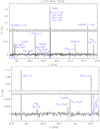 |
Fig. 2 Upper and lower panels: IRAM-WideX spectra (in Fν scale) extracted at the L1157-B1b blueshifted position (see Fig. 1 and text). The spectral resolution is 1.95 MHz (see Sect. 3). A zoom-in in intensity is shown so that the weakest lines can be seen. The transitions producing the emission lines are labelled in blue, with the corresponding frequencies marked by vertical blue lines. The detected CH3OH and CH3COH lines (analysed here) are reported in Table 1. |
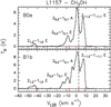 |
Fig. 3 CH3OH emission spectra at 96.7 GHz (in TB scale) extracted at the B0e and B1b positions (see Fig. 1 and text). The spectral resolution is 0.48 MHz, corresponding to 0.16 km s−1. The transitions producing the emission lines (see Table 1) are reported, with the corresponding frequencies marked by small vertical red lines. The spectra are centred at the frequency of the 20,2 − 10,1 A transition: 96 741.38 MHz. The dashed vertical line stands for the systemic velocity: +2.6 km s−1 (e.g. Bachiller et al. 2001). |
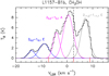 |
Fig. 4 Spectral fit of the 2-1,2–1-1,1 E (grey lines), 20,2–10,1 A (magenta), and 20,2–10,1 E (blue) triplets as observed towards B1b using the NOEMA narrow-band spectrometer. The spectra are centred at the frequency of the 20,2–10,1 A transition: 96 741.38 MHz. The transitions producing the emission lines (see Table 1) are reported, with the corresponding frequencies marked by small vertical red lines. The dashed vertical line is for the systemic velocity: +2.6 km s−1 (e.g. Bachiller et al. 2001). Each transition shows a main peak at +0.5 km s−1 plus a secondary peak further blueshifted by ~5 km s−1. |
4.3 Large Velocity Gradient analysis and rotational diagrams: column densities and abundances
Given the lack of CH3CHO collisional rates in the literature, we only analysed the CH3OH emission with the non-local thermodinamic equilibrium (NLTE) large velocity gradient (LVG) approach using the model described in Ceccarelli et al. (2003). We used the CH3OH-H2 collisional coefficients computed by Rabli & Flower (2010) and provided by the BASECOL database (Dubernet et al. 2013). In the computations, we assumed a H2 ortho-to-para ratio of one (Nisini et al. 2010). We run grids of models varying the kinetic temperature (Tkin) from 50 to 300 K, the volume density (nH2) from 104 to 108 cm−3, and the methanol column density (N(CH3OH)) from 1014 to 1018 cm−2. The best fit is obtained by the minimum χ2 in the three parameters. The errors on the observed line intensities have been obtained by propagating the spectral rms with the uncertainties due to calibration (15%).
Figure 5 shows: (i) the χ2 contour plot in the Tkin–nH2 plane obtained with the best fit of the methanol column density N(CH3OH) = 5 × 1015 cm−2 (3–8 × 1015 cm−2, including uncertainties), (ii) the χ2 –N(CH3OH) distribution, where it is possible to identify the minimum χ2 value (2.4), and (iii) the ratio between the measured and predicted intensity of the observed lines. Overall, the best fit is very good, with a reduced χ2 equal to 1.2, which for two degrees of freedom corresponds to a probability of 30% to exceeding χ2 (i.e. approximately the standard 1 σ). The methanol line opacities are predicted to be less than 0.1. The volume density is well constrained, nH2 = 4 × 105 cm−3 (2–10 × 105 cm−3), in agreement with the high densities (≥ 105 cm−3) inferred toward the molecular cavities by Gómez-Ruiz et al. (2015) from a CS multiline analysis. The kinetic temperature is also well constrained, Tkin = 90 K (70–130 K), again in agreement with the temperatures of the B1 cavity as derived by Lefloch et al. (2012) using a CO multiline single-dish analysis. We note that a recent LVG analysis of methanol emission as observed using single-dish towards a large number of protostellar jet-driven shocks (Holdship et al. 2019) shows volume densities in the 105 –106 cm−3 range and kinetic temperatures between 20 and 60 K, values consistent with what is found in L1157-B1.
The analysis described immediately above allows us to constrain the density and temperature of the methanol-emitting gas. However, in order to derive the relative abundances of methanol and acetaldehyde, we carried out a rotational diagram (RD) analysis for both molecules, where a LTE population and optically thin lines are assumed (in agreement with the NLTE LVG analysis of methanol described above). Under these assumptions, for a given molecule, the relative population distribution of all the energy levels is described by a Boltzmann temperature, that is the rotational temperature Trot. As demonstrated by Lefloch et al. (2012), for example, by analysing CO emission from extended outflowing gas in L1157, the column density obtained with RD gives results that are in relatively good agreement with a NLTE LVG analysis, usually within a factor two, as is also the case for our analysis.
Figure 6 shows the RD of CH3OH, which provides a column density of (1.3 ± 0.3) × 1016 cm−2, close to what was found using the LVG method. The rotational temperature is (10.0 ± 1.1) K, in agreement with what was found using previous interferometric and single dish measurements of CH3OH lines in the same excitation range (12 K; Bachiller et al. 1995; Benedettini et al. 2007; Codella et al. 2010). Thanks to the many CH3CHO detected lines (covering an upper level energy Eu range similar to that traced by the methanol lines) we can carry out the RD analysis also for acetaldehyde, obtaining, as for CH3OH, a low rotational temperature, (8 ± 1) K, and a total column density N(CH3CHO) = (7±3) × 1013 cm−2. Lefloch et al. (2017) report for CH3CHO a rotationaltemperature of 17 K, but this was measured including transitions with Eu up to 94 K. Figure 7 shows the spatial distribution of the CH3CHO (upper panel) and CH3OH (lower panel) rotational temperature in the B0 and B1 regions of the L1157 outflow. We note that the CH3CHO rotational temperature map covers a smaller portion of the L1157 region due to the weakness of the acetaldehyde lines with Eu = 23 K. Considering the uncertainties (B0e and B1e: ~6 K; B1b: ~3 K) there is no significant difference between the rotational temperature of the two species or spatial trends throughout the L1157-B1 structure.
Finally, we computed the abundances of the various species using the values of their respective column densities divided by the H2 column density, which was derived from the CO column density in the B1 molecular cavity (NCO = 2 × 1017 cm−2: Lefloch et al. (2012) assuming the standard [CO]/[H] = 5 × 10⁻⁵ value. In this way, we obtain methanol and acetaldehyde abundances with respect to H equal to 6.5 × 10⁻⁶ (1.2–12 × 10−6, considered the uncertainties) and 3.5 × 10⁻⁸ (2–5 × 10⁻⁶), respectively,in good agreement with that derived by CC17 for acetaldehyde (1–3 × 10⁻⁸) using a coarser angular resolution (5′′ –6′′).
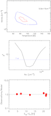 |
Fig. 5 Upper panel: density-temperature contour plot of χ2 obtained considering the non-LTE LVG-model-predicted and observed intensity of all the A and E CH3 OH emission lines detected (beam averaged) towards the B1b clump. The best fit is obtained with N(CH3OH) = 5 × 1015 cm−2, Tkin = 90 K, and nH2 = 4 × 105 cm−3. Middle panel: χ2 –N(CH3OH) distribution,identifying the minimum χ2 value (2.4). Lower panel: ratio between observations and model predictions of the CH3 OH A (circles) and E (stars) line intensities as a function of the upper level energy of the lines. |
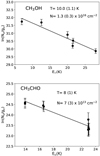 |
Fig. 6 Rotational diagrams for CH3OH (upper panel), and CH3CHO (lower panel) derived using the emission lines observed towards B1b (see Table 1 and Fig. 3). The parameters Nu, gu, and Eup are the column density, the degeneracy, and the energy (with respect to the ground state of each symmetry), respectively, of the upperlevel. The derived values of the rotational temperature are reported in the panels. |
5 Discussion
5.1 The CH3OH to CH3CHO abundance ratio
Codella et al. (2017) showed that the spatial distribution of the measured abundance ratio of iCOMs can lead to very stringent constraints on how they are formed and destroyed. In particular, these latter authors showed that the formamide to acetaldehyde abundance ratio towards the L1157-B1 shock demonstrates a gas-phase formation route of formamide (e.g. Skouteris et al. 2017). Further analysis of the abundance ratio of acetaldehyde with respect to methanol is therefore worthwhile, which can be safely assumed to form on dust mantles and then injected into the gas phase. Based on the interferometric maps showing that both species are populating the same gas portion, the ratio between their column densities can be used to derive their abundance ratio. The ratio of CH3OH to CH3CHO is about 1.5 × 10² and 1.9 × 10² as measured towards the B0e and B1b peaks, respectively, and it varies by less than a factor of three throughout the whole B0–B1 structure, as shown in Fig. 8. Considering that the uncertainty on these measurements is about 30%, there is no evidence for significant variation of this latter ratio in the observed region. Furthermore, these measurements are consistent with those derived using the ASAI IRAM 30 m single-dish survey (1–3 × 10² ; Codella et al. 2015; Lefloch et al. 2017). We note that Holdship et al. (2019) measured CH3OH/CH3CHO abundance ratios towards a sample of shocks using the IRAM 30 m antenna, finding higher values (by a factor of six on average): 0.4–1.3 × 10³ ; high-spatial-resolution surveys are needed to confirm these values.
It is interesting to check whether the CH3OH/CH3CHO abundance ratios derived for L1157-B0 and L1157-B1 are different with respect to measurements towards known Class 0 hot corinos, which rather trace the inner 100 au from the protostar where the temperature is high enough (at least 100 K) to thermally evaporate the dust-mantle products into the gas phase, or where grain mantles are sputtered by shocks (see below). If we only include in the comparison those sources imaged with high-spatial-resolution interferometric observations (to be sure of a proper comparison between the CH3OH and CH3CHO spatial distributions), the sample size is limited (see Table 2): HH212-mm (Lee et al. 2017, 2019; Bianchi et al. 2017; Codella et al. 2018), IRAS 16293-2422B (Jørgensen et al. 2016, 2018), NGC 1333-IRAS 4A2 (López-Sepulcre et al. 2017), Barnard 1b–S (Marcelino et al. 2018), and L483 (Jacobsen et al. 2018). Table 2 shows that the CH3OH/CH3CHO ratio of the hot-corinos varies from ~90 to ~500, that is, by less than a factor of six. The L1157 values fall inside this range, suggesting that the chemistry at work in the protostellar shocks, at least in the CH3OH and CH3CHO context, is similar to that ruling in the inner 100 au of the protostellar region. Of course, this is speculation based on one shocked region, and verification is required: (i) by increasing similar measurements towards different outflow shocks, and (ii) by investigating whether the chemical enrichment around a protostar is ruled by thermal evaporation or sputtering due to accretion shocks (see e.g. Sakai et al. 2014a,b; Lee et al. 2017, 2019; Codella et al. 2018).
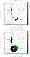 |
Fig. 7 CH3CHO (upper panel) and CH3OH (lower panel) rotational temperature (Trot) map (in K scale) of the B0 and B1 region of the L1157 outflow (derived from the NOEMA images, where the emission is at least 3σ), overlaid on the CO (black contours; Gueth et al. 1996) emission map. Uncertainties on Trot are ~ 3 K towards B1b, and ~6 K for B1e and B0. Symbols are as in Fig. 1. |
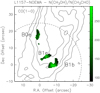 |
Fig. 8 Map of the ratio between the CH3OH and CH3CHO column density of the B0 and B1 region of the L1157 outflow (derived from the NOEMA images, where the emission is at least 3σ), overlaid on the CO (black contours; Gueth et al. 1996) emission map. Uncertainties are ≃ 30% (i.e. 30–100 in absolute values). Symbols are as in Fig. 1. |
Comparison of the CH3OH/CH3CHO abundance ratio as derived towards L1157-B1 with those measured towards Class 0 hot corinos using interferometric observations.
5.2 Chemical modelling
The overlap between the spatial distribution of the CH3OH and CH3CHO emission suggests that either acetaldehyde or a parent molecule was previously formed on the grain mantles, such as methanol for example, and was injected into the gas because of the passage of the shock. In addition, given that the CH3OH/CH3CHO abundance ratio is similar in the B0 and B1 knots despite them having a different kinematical age of less than about 1000 yr, if CH3CHO is synthesised in the gas phases, the process must be relatively fast. We note that recently, Burkhardt et al. (2019) modelled the shocked chemistry in L1157-B1 finding that CH3CHO has a post-shock chemistry due to sputtering, and additionally that a significant amount of its formation is due to gas-phase processes before 103 yr. The goalof this section is to explore whether gas-phase reactions are indeed fast enough to be able to reproduce the observations.
To this end, we used the same astrochemical model adopted in CC17 to analyse the formamide and acetaldehyde emission towards L1157-B1. The full details of the model can be found in CC17. Briefly, we used the time-dependent model gas-phase code MyNahoon, and adopteda two-step procedure: (1) we first compute the chemical composition of a standard molecular cloud at 10 K with a H2 density of 2 × 104 cm−3 and initial elemental abundances as in Agundez & Wakelam (2013, their Table 3). (2) We then successively increase the gas temperature, density, and gaseous abundance of grain-mantle species to simulate the shock passage. The gas temperature and H2 density are taken as those found by the NLTE LVG modelling, namely 90 K and 4 × 105 cm−3, respectively. For the abundances of the species injected into the gas phase at the moment of the passage of the shock, when possible, we assumed abundances (with respect to H nuclei) similar to those measured by IR observations of the interstellar dust ices (Boogert et al. 2015): CO2 (3 × 10⁻⁵) and H2 O (2 × 10⁻⁴; see also Busquet et al. 2014). Otherwise, we used the values constrained by previous studies on the L1157-B1 chemistry: OCS (2 × 10⁻⁶; Podio et al. 2014), NH3 (2 × 10⁻⁵; Tafalla & Bachiller 1995). We varied the injected CH3CH2 abundance in the gas-phase acetaldehyde formation model so as to obtain the observed acetaldehyde abundance. We found it necessary to inject CH3CH2/H = 8 × 10⁻⁸. Similarly, in the grain-surface acetaldehyde formation model, we modified the acetaldehyde abundances to fit the measured value in B1b (see Sect. 4.3), namely we assumed CH3CHO/H = 3.5 × 10⁻⁸. Finally, in both models, methanol is assumed to be a grain-surface product and the abundance injected in the gas phase is equal to that observed, namely 6.5 × 10⁻⁶ (see Sect. 4.3).
As in CC2017, we run both the case where acetaldehyde is directly injected into the gas phase from the grain mantles and the case in which it is formed in the gas phase, mainly by the reaction of ethyl radical (CH3CH2) with atomic oxygen: CH3CH2 + O → CH3CHO + H, as suggested by Charnley et al. (2004). With respect to the chemical network used by CC2017, we included the recent theoretical study by Gao et al. (2018) on the destruction of methanol by the reaction with OH.
Figure 9 reports the model predictions as a function of time after the shock passage compared with the values measured towards B1b. As written above, if acetaldehyde is directly sputtered from the grain mantles, in order to fit the observations, its injected abundance must be equal to 3.5 × 10⁻⁸. On the other hand, if acetaldehyde is formed via gas-phase reactions, the injected ethyl radical abundance must be 8 × 10⁻⁸. As shown in the figure, the gas phase reactions are relatively fast at synthesising acetaldehyde: within 300 yr the acetaldehyde abundance reaches its peak, after which it slowly decreases because of the destruction from ions in the gas phase, on a timescale larger than about 2000 yr. Therefore, it is impossible to elucidate the formation route of acetaldehyde in L1157-B1: a similar study towards an even younger shock might be able to shed light on the question. Alternatively, a less dense shock region, or one that was less irradiated by cosmic rays could be good site for better constraining the acetaldehyde formation route, as the chemical evolution would be slowed down in those cases.
As a final remark, we would like to highlight the fact that, although relatively simple, the modelling described above and used in this work catches the basic processes at work after the passage of a shock and has proven to be relatively reliable for reproducing the observations (see e.g. Podio et al. 2014 and C2017). The most drastic shortcoming of our model compared to more accurate and/or sophisticated shock models is its lack of a higher temperature (up to 1000 K) over a short(a few hundred years at most) period (see e.g. Viti et al. 2011). This could be important in the presence of species whose abundances depend on reactions with activation barriers that make them inefficient at low (≤100 K) temperatures but efficient at higher ones. In the specific case modelled here, we verified that no similar reactions are present and that a high-temperature (1000 K) phase does not impact our results.
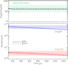 |
Fig. 9 Model predictions of methanol and acetaldehyde after a shock passage. Upper panel: CH3 OH/CH3CHO abundance ratio: solid line refers to a model where acetaldehyde is synthesised in the gas phase, whereas the dashed line refers to predictions assuming that CH3 OH is injected into the gas phase directly from the grain mantles. The hatched green zone is defined by the value (including uncertainty) measured towards the B1b peak, with a kinematical age of ≃ 1100 yr (Podio et al. 2016, revised according to the new distance of 352 pc by Zucker et al. 2019). Lower panel: acetaldehyde (CH3 CHO, red) and methanol (CH3OH, blue) abundances with respect to H nuclei as a function of time from the passage of the shock. The hatched blue and red regions show the measurements towards B1b (see text). |
6 Conclusions
In the context of the IRAM NOEMA SOLIS Large Program we imaged six methanol and eight acetaldehyde emission lines toward the B0 and B1 shocks along the L1157 blueshifted outflow. The measured abundances relative to H nuclei are 6.5 × 10⁻⁶ (methanol) and 3.5 × 10⁻⁸ (acetaldehyde). The CH3OH and CH3CHO spatial distributions overlap well, tracing the earliest shocked regions. Comparison with astrochemical model predictions shows that CH3CHO is either formed on the dust mantles or is quickly formed in the gas phase using simpler mantle products. Our modelling demonstrates that two species emitting lines in the same region is not enough to guarantee that they are grain-surface products: gas-phase reactions triggered by different species from the grain mantles could also display the same spatial behaviour. Detailed studies are required in order to discriminate between grain-surface and gas-phase chemistry as the major process leading to the observed species and to decipher the timescale on which this formation occurs.
For acetaldehyde in particular, at present, it is not possible to measure the abundance of one of the two parent species (ethyl radical) possibly synthesising acetaldehyde in the gas phase. The measurement of the second parent species, atomic oxygen, is challenging, as its fine structure line at 63 μm lies in a spectral window that is totally blocked by the terrestrial atmosphere. The SOFIA telescope could overcome this problem (Kristensen et al. (2017). On the other hand, although the frequencies (and spectroscopic parameters) of ethyl radicals are unknown at present, they would be a very welcome target of specific spectroscopic studies. It would then very likely be possible to search for ethyl radicals in regions where acetaldehyde is detected, and thus decipher whether or not the proposed gas-phase route is correct.
Acknowledgements
We are very grateful to all the IRAM staff, whose dedication allowed us to carry out the SOLIS project. This work was supported by (i) the PRIN-INAF 2016 “The Cradle of Life – GENESIS-SKA (General Conditions in Early Planetary Systems for the rise of life with SKA)”, (ii) the program PRIN-MIUR 2015 STARS in the CAOS – Simulation Tools for Astrochemical Reactivity and Spectroscopy in the Cyberinfrastructure for Astrochemical Organic Species (2015F59J3R, MIUR Ministero dell’Istruzione, dell’Università della Ricerca e della Scuola Normale Superiore), and (iii) the European Research Council (ERC) under the European Union’s Horizon 2020 research and innovation programme, for the Project “The Dawn of Organic Chemistry” (DOC), grant agreement No 741002.
Appendix A The NOEMA-SOLIS CH3OH and CH3CHO line maps
Figures A.1 and A.2 show the images of the detected CH3OH and CH3CHO emission lines (see Table 1). For comparison, the CO (1–0) (white contours; Gueth et al. 1996) and NH2CHO (41,4–31,3) (cyan contours; Codella et al. 2017) spatial distributions are also reported.
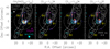 |
Fig. A.1 L1157 southern blueshifted lobe in CO (1–0) (white contours; Gueth et al. 1996) and NH2 CHO (41,4 –31,3) (cyan contours; Codella et al. 2017). The precessing jet ejected by the central object L1157-mm (outside the frame and toward the northwest) excavated several clumpy cavities, named B0, B1, and B2, respectively. The maps are centred at α(J 2000) = 20h 39m10s.2, δ(J 2000) = +68°01′10′′.5 (Δα = +25′′ and Δδ = –63′′.5 from the L1157-mm protostar). Map (in colour scale) of the sum of the CH3 OH (2-1,2 –1-1,1) E, (20,2 –10,1) A, and (20,2–10,1) E emission lines (labelled 2k,k–1k,k), (21,2 –11,1) A, (21,1–11,0) A, and (21,1–11,0) E (integrated over the whole velocity range). For the CO image, the first contour and step are 6σ (1σ = 0.5 Jy beam−1 km s−1) and 4σ, respectively. The first contour and step of the NH2CHO map (cyan contours) correspond to 3σ (15 mJy beam−1 km s−1) and 1σ, respectively. The dashed circle shows the primary beam of the CH3OH images (64′′). The first contour and step are 3σ (56, 32, 45, and 23 mJy beam−1 km s−1 for 2k,k –1k,k, 21,2 –11,1 A, 21,1 –11,0 A, and (21,1–11,0) E, respectively. Yellow labels are for the B0, B1, and B2 regions: the positions of the different clumps inside these regions are shown in Fig. 1 (see also text, and e.g. Codella et al. 2009, 2017). The cyan, white, and magenta ellipses depict the synthesised beams of the NH2 CHO (5′′.79 × 4′′.81, PA = –94°), CO (3′′.65 × 2′′.96, PA = +88°), and CH3OH (2′′.97 × 2′′.26, PA = –155°) observations, respectively. |
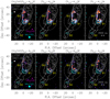 |
Fig. A.2 L1157 southern blueshifted lobe in CO (1–0) (white contours; Gueth et al. 1996) and NH2 CHO (41,4 –31,3) (cyan contours; Codella et al. 2017). The precessing jet ejected by the central object L1157-mm (outside the frame and toward the northwest) excavated several clumpy cavities, named B0, B1, and B2, respectively. The maps are centred at α(J 2000) = 20h 39m10s.2, δ(J2000) = +68°01′10′′.5 (Δα = +25′′ and Δδ = –63′′.5 from L1157-mm). For the CO image, the first contour and step are 6σ (1σ = 0.5 Jy beam−1 km s−1) and 4σ, respectively. The first contour and step of the NH2CHO map (cyan contours) correspond to 3σ (15 mJy beam−1 km s−1) and 1σ, respectively. The dashed circle shows the primary beam of the CH3CHO images(64′′). Upper panels: map (in colour scale) of line emission (integrated over the whole velocity range) due to CH3 CHO (50,4 –40,4) E, (50,4 –40,4) A, (51,4–41,3) E, and (51,4–41,3) A, respectively. The first contour and step are 3σ: 7 mJy beam−1 km s−1 (50,4 –40,4 E, 50,4 –40,4 A), and 8 mJy beam−1 km s−1 (51,4 –41,3 E, and 51,4–41,3 A). The cyan, white, and magenta ellipses depict the synthesised beams of the NH2 CHO (5′′.79 × 4′′.81, PA = –94°), CO (3′′.65 × 2′′.96, PA = +88°), and CH3CHO (2′′.97 × 2′′.26, PA = –155°) observations, respectively). Yellow labels are for the B0, B1, and B2 regions: the positions of the different clumps inside these regions are shown in Fig. 1 (see also text, and e.g. Codella et al. 2009, 2017). Lower panels: same as upper panels but for the CH3 CHO (52,4 –42,3) A, (52,4–42,3) E, (52,3 –52,2) E, and (52,3–42,2) A. The first contour and step are 3σ: 5 mJy beam−1 km s−1 for 52,4 –42,3 A,E, and 4 mJy beam−1 km s−1 for 52,3 –52,2 A,E. |
References
- Agundez, M., & Wakelam, V. 2013, Chem. Rev., 113, 8710 [CrossRef] [PubMed] [Google Scholar]
- Arce, H. G., Santiago-García, J., Jørgensen, J. K., Tafalla, M., & Bachiller, R. 2008, ApJ, 681, L21 [NASA ADS] [CrossRef] [Google Scholar]
- Bachiller, R., Liechti, S., Walmsley, C. M., & Colomer, F. 1995, A&A, 295, L51 [NASA ADS] [Google Scholar]
- Bachiller, R., Peréz Gutiérrez, M., Kumar, M. S. N., & Tafalla, M. 2001, A&A, 372, 899 [NASA ADS] [CrossRef] [EDP Sciences] [Google Scholar]
- Balucani, N., Ceccarelli, C., & Taquet, V. 2015, MNRAS, 449, L16 [Google Scholar]
- Burkhardt, A. M., Shingledeker, C. N., Le Gal, R., et al. 2019, ApJ, 881, 32 [NASA ADS] [CrossRef] [Google Scholar]
- Belloche, A., Garrod, R. T., Müller, H. S. P., & Menten, K. M. 2014, Science, 345, 1584 [NASA ADS] [CrossRef] [PubMed] [Google Scholar]
- Benedettini, M., Viti, S., Codella, C., et al. 2007, MNRAS, 381, 1127 [NASA ADS] [CrossRef] [Google Scholar]
- Benedettini, M., Viti, S., Codella, C., et al. 2013, MNRAS, 436, 179 [NASA ADS] [CrossRef] [Google Scholar]
- Bianchi, E., Codella, C., Ceccarelli, C., et al. 2017, A&A, 606, L7 [NASA ADS] [CrossRef] [EDP Sciences] [Google Scholar]
- Boogert, A. C. A., Gerakines, P. A., & Whittet, D. C. B. 2015, ARA&A, 53, 541 [Google Scholar]
- Busquet, G., Lefloch, B., Benedettini, M., et al. 2014, A&A, 561, A120 [NASA ADS] [CrossRef] [EDP Sciences] [Google Scholar]
- Caselli, P., & Ceccarelli, C. 2012, A&ARv, 20, 56 [NASA ADS] [CrossRef] [MathSciNet] [Google Scholar]
- Caselli, P., Hartquist, T. W., & Havnes, O. 1997, A&A, 322, 286 [Google Scholar]
- Ceccarelli, C., Maret, S., Tielens, A. G. G. M., Castets, A., & Caux, E. 2003, A&A, 410, 587 [NASA ADS] [CrossRef] [EDP Sciences] [Google Scholar]
- Ceccarelli, C., Caselli, P., Fontani, F., et al. 2017, ApJ, 850, 176 [NASA ADS] [CrossRef] [Google Scholar]
- Charnley, S. B. 2004, Adv. Space Res., 33, 23 [Google Scholar]
- Charnley, S. B., Tielens, A. G. G. M., & Millar, T. J. 1992, ApJ, 399, L71 [NASA ADS] [CrossRef] [Google Scholar]
- Codella, C., Benedettini, M., Beltrán, M. T., et al. 2009, A&A, 507, L25 [NASA ADS] [CrossRef] [EDP Sciences] [Google Scholar]
- Codella, C., Lefloch, B., Ceccarelli, C., et al. 2010, A&A, 518, L112 [NASA ADS] [CrossRef] [EDP Sciences] [Google Scholar]
- Codella, C., Fontani, F., Ceccarelli, C., et al. 2015, MNRAS, 449, L11 [NASA ADS] [CrossRef] [Google Scholar]
- Codella, C., Ceccarelli, C., Caselli, P., et al. 2017, A&A, 605, L3 [NASA ADS] [CrossRef] [EDP Sciences] [Google Scholar]
- Codella, C., Bianchi, E., Tabone, B., et al. 2018, A&A, 617, A10 [NASA ADS] [CrossRef] [EDP Sciences] [Google Scholar]
- Dubernet, M. L., Alexander, M. H., Ba, Y. A., et al. 2013, A&A, 553, A50 [NASA ADS] [CrossRef] [EDP Sciences] [Google Scholar]
- Flower, D. R., & Pineau des Forêts, G. 1994, MNRAS, 268, 724 [NASA ADS] [CrossRef] [Google Scholar]
- Fontani, F., Codella, C., Ceccarelli, C., et al. 2014, ApJ, 788, L43 [NASA ADS] [CrossRef] [Google Scholar]
- Gao, L. G., Zheng, J., Fernández-Ramos, A., Truhlar, D. G., & Xu, X. 2018, J. Am. Chem. Soc., 140, 8 [Google Scholar]
- Garrod, R. T., & Herbst, E. 2006, A&A, 457, 927 [NASA ADS] [CrossRef] [EDP Sciences] [Google Scholar]
- Garrod, R. T., Widicus Weaver, S. L., & Herbst, E. 2008, ApJ, 682, 283 [NASA ADS] [CrossRef] [Google Scholar]
- Gómez-Ruiz, A. I., Codella, C., Lefloch, B., et al. 2015, MNRAS, 446, 3346 [NASA ADS] [CrossRef] [Google Scholar]
- Gueth, F., Guilloteau, S., & Bachiller, R. 1996, A&A, 307, 891 [NASA ADS] [Google Scholar]
- Gueth, F., Guilloteau, S., & Bachiller, R. 1998, A&A, 333, 287 [NASA ADS] [Google Scholar]
- Gusdorf, A., Cabrit, S., Flower, D. R., & Pineau des Forêts, G. 2008a, A&A, 482, 809 [Google Scholar]
- Gusdorf, A., Pineau des Forêts, G., Cabrit, S., & Flower, D. R. 2008b, A&A, 490, 695 [NASA ADS] [CrossRef] [EDP Sciences] [Google Scholar]
- Holdship, J., Viti, S., Codella, C., et al., 2019, ApJ, 880, 138 [NASA ADS] [CrossRef] [Google Scholar]
- Herbst, E., & van Dishoeck, E. F. 2009, ARA&A, 47, 427 [NASA ADS] [CrossRef] [Google Scholar]
- Jacobsen, S. K., Jørgensen, J. K., Di Francesco, et al. 2018, A&A, 629, A29 [Google Scholar]
- Jørgensen, J. K., van der Wiel, M. H. D., Coutens, A., et al. 2016, A&A, 595, A117 [NASA ADS] [CrossRef] [EDP Sciences] [Google Scholar]
- Jørgensen, J. K., Müller, H. S. P., Calcutt, H., et al. 2018, A&A, 620, A170 [NASA ADS] [CrossRef] [EDP Sciences] [Google Scholar]
- Kristensen, L. E., Gusdorf, A., Mottram, J. C., et al. 2017, A&A, 601, L4 [CrossRef] [EDP Sciences] [Google Scholar]
- Lee, C.-F., Li, Z.-Y., Ho, P.-T.-P., et al. 2017, ApJ, 843, L27 [NASA ADS] [CrossRef] [Google Scholar]
- Lee, C.-F., Codella, C., Li, Z.-Y., & Liu, S.-Y. 2019, ApJ, 873 L63 [NASA ADS] [CrossRef] [Google Scholar]
- Lefloch, B., Cabrit, S., Busquet, G., et al. 2012, ApJ, 757, L25 [NASA ADS] [CrossRef] [Google Scholar]
- Lefloch, B., Ceccarelli, C., Codella, C., et al. 2017, MNRAS, 469, L73 [NASA ADS] [CrossRef] [Google Scholar]
- Lefloch, B., Bachiller, R., Ceccarelli, C., et al. 2018, MNRAS, 477, 4792 [NASA ADS] [CrossRef] [Google Scholar]
- López-Sepulcre, A., Sakai, N., Neri, R., et al. 2017, A&A, 606, A121 [NASA ADS] [CrossRef] [EDP Sciences] [Google Scholar]
- Marcelino, N., Gerin, M., Cernicharo, J., et al. 2018, A&A, 620, A80 [NASA ADS] [CrossRef] [EDP Sciences] [Google Scholar]
- Mendoza, E., Lefloch, B., López-Sepulcre, A., et al. 2014, MNRAS, 445, 151 [NASA ADS] [CrossRef] [MathSciNet] [Google Scholar]
- Nisini, B., Benedettini, B., Codella, C., et al. 2010, A&A, 518, L120 [NASA ADS] [CrossRef] [EDP Sciences] [Google Scholar]
- Pickett, H. M., Poynter, R. L., Cohen, E. A., et al. 1998, J. Quant. Spectr. Rad. Transf., 60, 883 [NASA ADS] [CrossRef] [Google Scholar]
- Podio, L., Lefloch, B., Ceccarelli, C., Codella, C., & Bachiller, R. 2014, A&A, 565, A64 [NASA ADS] [CrossRef] [EDP Sciences] [Google Scholar]
- Podio, L., Codella, C., Gueth, F., et al. 2016, A&A, 593, L4 [NASA ADS] [CrossRef] [EDP Sciences] [Google Scholar]
- Rabli, D., & Flower, D. R. 2010, MNRAS, 406, 95 [NASA ADS] [CrossRef] [Google Scholar]
- Rimola, A., Taquet, V., Ugliengo, P., Balucani, N., & Ceccarelli, C. 2014, A&A, 572, A70 [NASA ADS] [CrossRef] [EDP Sciences] [Google Scholar]
- Ruaud, M., Loison, J. C., Hickson, K. M., et al. 2015, MNRAS, 447, 4004 [NASA ADS] [CrossRef] [Google Scholar]
- Sakai, N., Sakai, T., Hirota, T., et al. 2014a, Nature, 507, 78 [NASA ADS] [CrossRef] [Google Scholar]
- Sakai, N., Oya, Y., Sakai, T., et al. 2014b, ApJ, 791, L38 [NASA ADS] [CrossRef] [Google Scholar]
- Schilke, P., Walmsley, C. M., Pineau des Forêts, G., & Flower, D. R. 1997, A&A, 321, 293 [NASA ADS] [Google Scholar]
- Skouteris, D., Vazart, F., Ceccarelli, C., et al. 2017, MNRAS, 468, L1 [NASA ADS] [Google Scholar]
- Skouteris, D., Balucani, N., Ceccarelli, C., et al. 2018, ApJ, 854, 135 [Google Scholar]
- Tafalla, M., & Bachiller, R. 1995, ApJ, 443, L37 [Google Scholar]
- Taquet, V., López-Sepulcre, A., Ceccarelli, C., et al. 2015, ApJ, 804, 81 [NASA ADS] [CrossRef] [Google Scholar]
- Tielens, A. G. G. M., & Hagen, W. 1982, A&A, 114, 245 [Google Scholar]
- Vasyunin, A. I., Caselli, P., Dulieu, F., & Jiménez-Serra, I. 2017, ApJ, 842, 33 [Google Scholar]
- Viti, S., Jimenez-Serra, I., Yates, J., et al. 2011, ApJ, 740, L3 [NASA ADS] [CrossRef] [Google Scholar]
- Watanabe, N., & Kouchi, A. 2002, ApJ, 571, L173 [NASA ADS] [CrossRef] [Google Scholar]
- Zucker, C., Speagle, J. S., Schlafly, E. F., et al. 2019, ApJ, 879, 125 [NASA ADS] [CrossRef] [Google Scholar]
All Tables
Comparison of the CH3OH/CH3CHO abundance ratio as derived towards L1157-B1 with those measured towards Class 0 hot corinos using interferometric observations.
All Figures
|
Fig. 1 L1157 southern blueshifted lobe in CO (1–0) (white contours; Gueth et al. 1996). The precessing jet ejected by the central object L1157-mm (outside the frame and toward the northwest) excavated several clumpy cavities, named B0, B1, and B2, respectively. The maps are centred at α(J2000) = 20h39m10s.2, δ(J2000) = + 68°01′10′′.5 (Δα = +25′′ and Δδ = −63′′.5 from the L1157-mm protostar). Top panel: map (in colour scale) of the emission due to the CH3 OH(21,2–11,1) A transition (integrated over the whole velocity range). The first contour and step are 3σ (32 mJy beam−1 km s−1). For the CO image, the first contour and step are 6σ (1σ = 0.5 Jy beam−1 km s−1) and 4σ, respectively. The dashed circle shows the primary beam of the CH3OH image (64′′). Yellow labels are for the B0 and B1 clumps (black triangles) previously identified using molecular tracers (see text, and e.g. Benedettini et al. 2007; Codella et al. 2009, 2017). The white and magenta ellipses depict the synthesised beams of the CO (3′′.65×2′′.96, PA = +88°), and CH3 OH (2′′.97×2′′.26, PA = –155°) observations, respectively. Bottom panel: same as top panel but for CH3CHO (50,4 –40,4) E. The first contour and step are 3σ (7 mJy beam−1 km s−1). The synthesised beams of the CH3CHO image are similar to those of the CH3OH map. |
| In the text | |
|
Fig. 2 Upper and lower panels: IRAM-WideX spectra (in Fν scale) extracted at the L1157-B1b blueshifted position (see Fig. 1 and text). The spectral resolution is 1.95 MHz (see Sect. 3). A zoom-in in intensity is shown so that the weakest lines can be seen. The transitions producing the emission lines are labelled in blue, with the corresponding frequencies marked by vertical blue lines. The detected CH3OH and CH3COH lines (analysed here) are reported in Table 1. |
| In the text | |
|
Fig. 3 CH3OH emission spectra at 96.7 GHz (in TB scale) extracted at the B0e and B1b positions (see Fig. 1 and text). The spectral resolution is 0.48 MHz, corresponding to 0.16 km s−1. The transitions producing the emission lines (see Table 1) are reported, with the corresponding frequencies marked by small vertical red lines. The spectra are centred at the frequency of the 20,2 − 10,1 A transition: 96 741.38 MHz. The dashed vertical line stands for the systemic velocity: +2.6 km s−1 (e.g. Bachiller et al. 2001). |
| In the text | |
|
Fig. 4 Spectral fit of the 2-1,2–1-1,1 E (grey lines), 20,2–10,1 A (magenta), and 20,2–10,1 E (blue) triplets as observed towards B1b using the NOEMA narrow-band spectrometer. The spectra are centred at the frequency of the 20,2–10,1 A transition: 96 741.38 MHz. The transitions producing the emission lines (see Table 1) are reported, with the corresponding frequencies marked by small vertical red lines. The dashed vertical line is for the systemic velocity: +2.6 km s−1 (e.g. Bachiller et al. 2001). Each transition shows a main peak at +0.5 km s−1 plus a secondary peak further blueshifted by ~5 km s−1. |
| In the text | |
|
Fig. 5 Upper panel: density-temperature contour plot of χ2 obtained considering the non-LTE LVG-model-predicted and observed intensity of all the A and E CH3 OH emission lines detected (beam averaged) towards the B1b clump. The best fit is obtained with N(CH3OH) = 5 × 1015 cm−2, Tkin = 90 K, and nH2 = 4 × 105 cm−3. Middle panel: χ2 –N(CH3OH) distribution,identifying the minimum χ2 value (2.4). Lower panel: ratio between observations and model predictions of the CH3 OH A (circles) and E (stars) line intensities as a function of the upper level energy of the lines. |
| In the text | |
|
Fig. 6 Rotational diagrams for CH3OH (upper panel), and CH3CHO (lower panel) derived using the emission lines observed towards B1b (see Table 1 and Fig. 3). The parameters Nu, gu, and Eup are the column density, the degeneracy, and the energy (with respect to the ground state of each symmetry), respectively, of the upperlevel. The derived values of the rotational temperature are reported in the panels. |
| In the text | |
|
Fig. 7 CH3CHO (upper panel) and CH3OH (lower panel) rotational temperature (Trot) map (in K scale) of the B0 and B1 region of the L1157 outflow (derived from the NOEMA images, where the emission is at least 3σ), overlaid on the CO (black contours; Gueth et al. 1996) emission map. Uncertainties on Trot are ~ 3 K towards B1b, and ~6 K for B1e and B0. Symbols are as in Fig. 1. |
| In the text | |
|
Fig. 8 Map of the ratio between the CH3OH and CH3CHO column density of the B0 and B1 region of the L1157 outflow (derived from the NOEMA images, where the emission is at least 3σ), overlaid on the CO (black contours; Gueth et al. 1996) emission map. Uncertainties are ≃ 30% (i.e. 30–100 in absolute values). Symbols are as in Fig. 1. |
| In the text | |
|
Fig. 9 Model predictions of methanol and acetaldehyde after a shock passage. Upper panel: CH3 OH/CH3CHO abundance ratio: solid line refers to a model where acetaldehyde is synthesised in the gas phase, whereas the dashed line refers to predictions assuming that CH3 OH is injected into the gas phase directly from the grain mantles. The hatched green zone is defined by the value (including uncertainty) measured towards the B1b peak, with a kinematical age of ≃ 1100 yr (Podio et al. 2016, revised according to the new distance of 352 pc by Zucker et al. 2019). Lower panel: acetaldehyde (CH3 CHO, red) and methanol (CH3OH, blue) abundances with respect to H nuclei as a function of time from the passage of the shock. The hatched blue and red regions show the measurements towards B1b (see text). |
| In the text | |
|
Fig. A.1 L1157 southern blueshifted lobe in CO (1–0) (white contours; Gueth et al. 1996) and NH2 CHO (41,4 –31,3) (cyan contours; Codella et al. 2017). The precessing jet ejected by the central object L1157-mm (outside the frame and toward the northwest) excavated several clumpy cavities, named B0, B1, and B2, respectively. The maps are centred at α(J 2000) = 20h 39m10s.2, δ(J 2000) = +68°01′10′′.5 (Δα = +25′′ and Δδ = –63′′.5 from the L1157-mm protostar). Map (in colour scale) of the sum of the CH3 OH (2-1,2 –1-1,1) E, (20,2 –10,1) A, and (20,2–10,1) E emission lines (labelled 2k,k–1k,k), (21,2 –11,1) A, (21,1–11,0) A, and (21,1–11,0) E (integrated over the whole velocity range). For the CO image, the first contour and step are 6σ (1σ = 0.5 Jy beam−1 km s−1) and 4σ, respectively. The first contour and step of the NH2CHO map (cyan contours) correspond to 3σ (15 mJy beam−1 km s−1) and 1σ, respectively. The dashed circle shows the primary beam of the CH3OH images (64′′). The first contour and step are 3σ (56, 32, 45, and 23 mJy beam−1 km s−1 for 2k,k –1k,k, 21,2 –11,1 A, 21,1 –11,0 A, and (21,1–11,0) E, respectively. Yellow labels are for the B0, B1, and B2 regions: the positions of the different clumps inside these regions are shown in Fig. 1 (see also text, and e.g. Codella et al. 2009, 2017). The cyan, white, and magenta ellipses depict the synthesised beams of the NH2 CHO (5′′.79 × 4′′.81, PA = –94°), CO (3′′.65 × 2′′.96, PA = +88°), and CH3OH (2′′.97 × 2′′.26, PA = –155°) observations, respectively. |
| In the text | |
|
Fig. A.2 L1157 southern blueshifted lobe in CO (1–0) (white contours; Gueth et al. 1996) and NH2 CHO (41,4 –31,3) (cyan contours; Codella et al. 2017). The precessing jet ejected by the central object L1157-mm (outside the frame and toward the northwest) excavated several clumpy cavities, named B0, B1, and B2, respectively. The maps are centred at α(J 2000) = 20h 39m10s.2, δ(J2000) = +68°01′10′′.5 (Δα = +25′′ and Δδ = –63′′.5 from L1157-mm). For the CO image, the first contour and step are 6σ (1σ = 0.5 Jy beam−1 km s−1) and 4σ, respectively. The first contour and step of the NH2CHO map (cyan contours) correspond to 3σ (15 mJy beam−1 km s−1) and 1σ, respectively. The dashed circle shows the primary beam of the CH3CHO images(64′′). Upper panels: map (in colour scale) of line emission (integrated over the whole velocity range) due to CH3 CHO (50,4 –40,4) E, (50,4 –40,4) A, (51,4–41,3) E, and (51,4–41,3) A, respectively. The first contour and step are 3σ: 7 mJy beam−1 km s−1 (50,4 –40,4 E, 50,4 –40,4 A), and 8 mJy beam−1 km s−1 (51,4 –41,3 E, and 51,4–41,3 A). The cyan, white, and magenta ellipses depict the synthesised beams of the NH2 CHO (5′′.79 × 4′′.81, PA = –94°), CO (3′′.65 × 2′′.96, PA = +88°), and CH3CHO (2′′.97 × 2′′.26, PA = –155°) observations, respectively). Yellow labels are for the B0, B1, and B2 regions: the positions of the different clumps inside these regions are shown in Fig. 1 (see also text, and e.g. Codella et al. 2009, 2017). Lower panels: same as upper panels but for the CH3 CHO (52,4 –42,3) A, (52,4–42,3) E, (52,3 –52,2) E, and (52,3–42,2) A. The first contour and step are 3σ: 5 mJy beam−1 km s−1 for 52,4 –42,3 A,E, and 4 mJy beam−1 km s−1 for 52,3 –52,2 A,E. |
| In the text | |
Current usage metrics show cumulative count of Article Views (full-text article views including HTML views, PDF and ePub downloads, according to the available data) and Abstracts Views on Vision4Press platform.
Data correspond to usage on the plateform after 2015. The current usage metrics is available 48-96 hours after online publication and is updated daily on week days.
Initial download of the metrics may take a while.