| Issue |
A&A
Volume 635, March 2020
|
|
|---|---|---|
| Article Number | A130 | |
| Number of page(s) | 14 | |
| Section | Interstellar and circumstellar matter | |
| DOI | https://doi.org/10.1051/0004-6361/201936394 | |
| Published online | 23 March 2020 | |
Protostellar disk formation by a nonrotating, nonaxisymmetric collapsing cloud: model and comparison with observations
1
Laboratoire AIM, Paris-Saclay, CEA Saclay/IRFU/DAp – CNRS – Université Paris Diderot,
91191
Gif-sur-Yvette Cedex,
France
e-mail: This email address is being protected from spambots. You need JavaScript enabled to view it.
2
LERMA (UMR CNRS 8112), Ecole Normale Supérieure,
75231
Paris Cedex,
France
3
Harvard-Smithsonian Center for Astrophysics,
60 Garden street,
Cambridge,
MA
02138,
USA
Received:
28
July
2019
Accepted:
3
February
2020
Abstract
Context. Planet-forming disks are fundamental objects that are thought to be inherited from large scale rotation through the conservation of angular momentum during the collapse of a prestellar dense core.
Aims. We investigate the possibility for a protostellar disk to be formed from a motionless dense core that contains nonaxisymmetric density fluctuations. The rotation is thus generated locally by the asymmetry of the collapse.
Methods. We study the evolution of the angular momentum in a nonaxisymmetric collapse of a dense core from an analytical point of view. To test the theory, we performed three-dimensional simulations of a collapsing prestellar dense core using adaptative mesh refinement. We started from a nonaxisymmetrical situation, considering a dense core with random density perturbations that follow a turbulence spectrum. We analyzed the emerging disk by comparing the angular momentum it contains with the one expected from our analytic development. We studied the velocity gradients at different scales in the simulation as is done with observations.
Results. We show that the angular momentum in the frame of a stellar object, which is not located at the center of mass of the core, is not conserved due to inertial forces. Our simulations of such nonaxisymmetrical collapse quickly produce accretion disks at the small scales in the core. The analysis of the kinematics at different scales in the simulated core reveals projected velocity gradients of amplitudes similar to the ones observed in protostellar cores and for which directions vary, sometimes even reversing when small and large scales are compared. These complex kinematics patterns appear in recent observations and could be a discriminating feature with models where rotation is inherited from large scales. Our results from simulations without initial rotation are more consistent with these recent observations than when solid-body rotation is initially imprinted. Lastly, we show that the disks that formed in this scenario of nonaxisymmetrical gravitational collapse grow to reach sizes larger than those that are observed, and then fragment. We show that including a magnetic field in these simulations reduces the size of the outcoming disks and it prevents them from fragmenting, as is shown by previous studies.
Conclusions. We show that in a nonaxisymmetrical collapse, the formation of a disk can be induced by small perturbations of the initial density field in the core, even in the absence of global large-scale rotation of the core. In this scenario, large disks are generic features that are natural consequences of the hydrodynamical fluid interactions and self-gravity. Since recent observations have shown that most disks are significantly smaller and have a size of a few tens of astronomical units, our study suggests that magnetic braking is the most likely explanation. The kinematics of our model are consistent with typically observed values of velocity gradients and specific angular momentum in protostellar cores. These results open a new avenue in which our understanding of the early phases of disk formation can be explored since they suggest that a fraction of the protostellar disks could be the product of nonaxisymmetrical collapse, rather than directly resulting from the conservation of preexisting large scale angular momentum in rotating cores.
Key words: methods: numerical / protoplanetary disks / ISM: clouds / ISM: kinematics and dynamics / turbulence / stars: formation
© A. Verliat et al. 2020
 Open Access article, published by EDP Sciences, under the terms of the Creative Commons Attribution License (http://creativecommons.org/licenses/by/4.0), which permits unrestricted use, distribution, and reproduction in any medium, provided the original work is properly cited.
1 Introduction
Protoplanetary disks are rotationally supported structures that form around young stars (Li et al. 2014; Dutrey et al. 2014; Testi et al. 2014). It is currently believed that the rotation of these disks is inherited from large scales of a few thousands of astronomical units, which is the scale of the parent prestellar dense core.
During the gravitational collapse of the core, if the angular momentum is conserved, the infalling material naturally forms a rotation dominated structure at the small scale of a hundred astronomical units. The rotation of the disk is thus inherited from the large scale angular momentum, and as a consequence, the velocity gradients at large and small scales are correlated. This scenario is extensively studied in the literature and, in particular, the majority of collapse calculations start with a prescribed rotation profile (see for example Bate 1998; Matsumoto & Hanawa 2003; Machida et al. 2005; Hennebelle & Fromang 2008). While reasonable, this scenario leads to the question regarding from which scale the angular momentum is inherited and how exactly this happens. Another frequent configuration consists in a cloud with a turbulent velocity field that is imprinted initially (Bate et al. 2003; Goodwin et al. 2004a,b; Dib et al. 2010; Hennebelle et al. 2016; Matsumoto et al. 2017; Gray et al. 2018; Kuznetsova et al. 2019). In this context as well, it has been found that disks form quickly. The usual interpretation is that the angular momentum is initially present because of the turbulence.
Observationally, the kinematics of the dense gas in both prestellar cores and protostellar envelopes has been studied thanks to the analysis of molecular line emission that has shown to harbor velocity gradients at scales of 0.01–0.1 pc, which is interpreted as the rotation of cores (see the early works by Goodman et al. 1993; Ohashi et al. 1997; Chen et al. 2007). The values of specific angular momentum measured inside protostellar envelopes at scales of a few thousand astronomical units are on average one order of magnitude lower than the ones observed at larger scales in starless structures (a few 10−4 km s−1 pc, see for example Belloche 2013; Yen et al. 2015a; Pineda et al. 2019 and the very recent work by Gaudel et al. 2020). More puzzling, however, are the observations showing that some protostellar cores show an apparent disorganization or even a reversal in their velocity pattern, which is sometimes interpreted as the contribution of infall motions to the projected velocity field (Tobin et al. 2011; Harsono et al. 2014) or counter rotation (Tobin et al. 2018; Takakuwa et al. 2018). Recent high dynamic range observations of a sample of 12 low-mass Class 0 protostars (in the CALYPSO sample) by Gaudel et al. (2020) exhibit systematic dispersion of velocity gradients between disks’ and envelopes’ scales, which puts the presence of large scale rotation into question. Moreover, observations of the specific angular momentum contained inT Tauri disks suggest that values are larger, by about one order of magnitude, than the specific angular momentum observed in the low-mass protostellar cores at scales of a few thousands astronomical units (Simon et al. 2000; Kurtovic et al. 2018; Pérez et al. 2018). These observations are hence difficult to reconcile with a simple picture of a rotating-infalling protostellar envelope for which conservation of angular momentum naturally produces a rotationally-supported disk in its center, and new models should be developed to reproduce these observations as well.
To tackle these issues, we investigate a scenario that also leads to the formation of a protostellar disk. Similar ideas as the ones exposed in this paper have already been developed in the context of spiral galaxy formation by Hoyle (1949), Sciama (1955), and Peebles (1969). In the context of protoplanetary disk formation, this paper is meant to be exploratory, so we used minimal physical ingredients. Our simulations are thus purely hydrodynamics, except in Sect. 4.6. We start from an extreme scenario, considering a perfectly motionless dense core with nonaxisymmetric density perturbations. The gravitational collapse of this core is thus nonaxisymmetric. We show analytically and numerically that this nonaxisymmetry leads to the possibility of generating rotation locally. As we start from an extreme motionless scenario, without considering velocity fluctuations, our model is not fully physical. Despite this fact, we then analyze the velocity gradients in our simulations and we reproduce the observational results from Gaudel et al. (2020) about the dispersion of velocity gradients. We show that the specific angular momentum step coincides with the results from Belloche (2013) and Gaudel et al. (2020). Our model thus exhibits good agreement with observational constraints on kinematics.
The plan of the paper is as follows. In the second section we present the theory that motivates our study, in the third section we present the numerical methods we used to investigate our problem, in the fourth and fifth sections we present the results obtained and discuss them, and the sixth section is the conclusion.
2 Theory
2.1 The axisymmetrical case
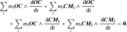
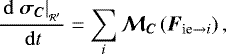
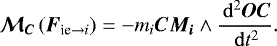
In the introduction, we evoke the conservation of angular momentum during the collapse of a dense core, leading to the formation of a disk. However, the angular momentum is correctly defined only in a given frame and with respect to a given point. We consider the angular momentum calculated in the simulation box frame  , with respect to the center O of this box1. It is computed as follows, with the summation referring to the different cells i of the simulation, mi and Mi are the mass and position of each cell i, respectively:
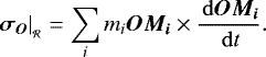 (1)
(1)
This momentum is conserved in virtue of the fundamental law of evolution of the angular momentum in a Galilean frame:
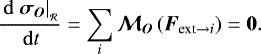 (2)
(2)
Since no external force is applied on the system, the angular momentum  is conserved. In a simple axisymmetrical case, this momentum coincides with what we call “the momentum of the disk”. Indeed, during the collapse, a disk forms in the center of the box, thus
  represents the angular momentum computed in the frame of the disk, in relation to the center of the disk.
2.2 Nonaxisymmetric configuration
In a nonaxisymmetrical case,  is no longer a relevant quantity to study the disk that formed in the simulation. In fact, to measure the angular momentum in protostellar disks, the reference point with respect to which the angular momentum is computed is the center of the disk, and the velocities considered are those in relation to the center of the disk, which are deduced from those projected on the line of sight (Belloche 2013). In the axisymmetrical case, the center of the formed disk remains motionless at the center of the simulation box. In the nonaxisymmetrical case, the disk is not formed at the center of the simulation box and it has a proper motion. We thus have to consider the angular momentum computed in the frame
  of the disk, in relation to the center C of the disk:
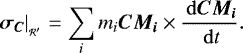 (3)
(3)
We show in Appendix A.1 that for an initial condition where all cells are at rest in  ,
,  can be expressed as:
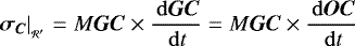 (4)
(4)
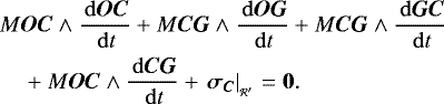
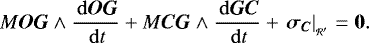
where  is the total mass of the system, and G is the center of mass2. Furthermore, the time derivative of Eq. (4) gives:
 (5)
(5)
This equation can be interpreted as the variation of the angular momentum  due to the torques of inertial force that apply to each cell of the simulation in the non-Galilean frame
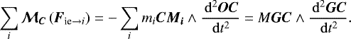
  (see Appendix A.2 for detailed development). Since the center of mass G and the center of the formed disk C do not coincide, the angular momentum
  is not expected to be conserved.
The point C is the accretion center of the system, and the matter collapses toward it. Since the angular momentum (in  with respect to C) of this matter does not vanish, a rotationally supported structure forms around C.
In the axisymmetrical case, the three points C, G, and O coincide as well as the two frames  and
and  . Thus
 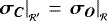 and the angular momentum is therefore conserved through the temporal evolution of the structure. In the nonaxisymmetrical case, Eq. (4) shows that the angular momentum
  is equal to the angular momentum of the point C to which the whole simulation mass has been allocated, which was computed with respect to G in the frame
  of the simulation box. Equation (5) shows that this angular momentum is not conserved in the general case. Here, we consider the extreme case where every cell is initially at rest in the simulation frame
  . We note that
  is thus initially null. As matter is falling toward the accretion center C, the transversal velocity of this matter has to increase for the angular momentum to grow. As a result, a rotational structure naturally forms around the accretion center without violating the conservation of the angular momentum in the simulation frame
  . These ideas are similar to those of Peebles (1969) who showed that the angular momentum of spiral galaxies can be understood as a consequence of tidal torques acting during the gravitational collapse.
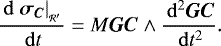
In our context of protostellar disk formation and before analyzing our simulations in Sect. 4.2 in detail, we can provide an order of magnitude for the expected momentum  . The simulations show that the distance between the points C and G is about a thousand astronomical units, which roughly corresponds to a tenth of the dense core radius, about 875 AU. The total mass inside the simulation is 2.5 M⊙. If we take the order of magnitude of the sound speed, 0.2 km s−1, for
  , we obtain:
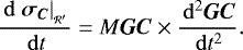
![Mathematical equation: \[ \left. \sigma_C \right| _{_{\mathcal{R'}}} \sim {2.5}~{{M}_{\odot}} ~\times~ {10^3}\,\textrm{AU} \times {0.2}\,\textrm{km\,s}^{-1} \sim {10^{47}}\textrm{kg\,m}^2\,\textrm{s}^{-1}. \]](/articles/aa/full_html/2020/03/aa36394-19/aa36394-19-eq28.png)
As is seen later, this order of magnitude is consistent with the values given by our analyses (see Fig. 3) and stresses good agreement with Belloche (2013) and Gaudel et al. (2020).
3 Numerical methods
3.1 Code and numerical parameters
To study whether the asymmetry of a gravitational collapse can be sufficient to form a prestellar disk, we carried out a set of hydrodynamics simulations with  AMSES (Teyssier 2002). This numerical Eulerian code uses the adaptative mesh refinement (AMR) technique to enhance resolution locally, where it is needed, on a Cartesian mesh. Our refinement criterion is based on Jeans length, such that each local Jeans length is described by at least 40 cells. We used ten levels of AMR, from 8 to 18, leading to a spatial resolution that goes from 270 to 0.26 AU.
3.2 Initial conditions
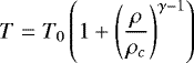
We consider a 3D cubic box with sides of 0.33 pc (about 70000 AU). In the middle of the box, we placed a 2.5 M⊙ sphere of gas that is the quarter of the box length in diameter and that has a flat radial density profile. This sphere acts as a model for the prestellar dense core. The rest of the box was filled with an envelop of gas whose density is constant and equal to a thousandth of the mean density of the gas sphere. Initially all velocities were set to zero so that the angular momentum in the box frame with respect to any motionless point was initially null. The alpha parameter, thermal over gravitational energy ratio, of the gas sphere is 0.35. We used a barotropic equation of state for the gas:
 (6)
(6)
in which T and ρ are the temperature and density of the gas, T0 = 10 K, ρc = 10−13g cm−3 is the critical density, and γ = 1.4 is the adiabatic index.
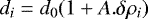
Since we wanted to study the effect of asymmetrical gravitational collapse, we broke the symmetry of the cloud by introducing random density perturbations in the dense core. To roughly mimic the physics of the interstellar gas, we based the probability distribution of the density perturbations on that of the turbulence (see for example Chapter 3 of Hennebelle & Falgarone 2012 for a review on turbulence in interstellar clouds). In the Fourier space, the perturbations spectrum matches with the power spectrum of the velocity for Kolmogorov turbulence3, and the phases are randomly chosen. We can thus write the density of each cell i of the prestellar core as:
 (7)
(7)
where d0 represents the mean density of the prestellar core, δρi is the value of the perturbation at the considered point, and ![Mathematical equation: $A \in \left[ 0, ~1 \right] $](/articles/aa/full_html/2020/03/aa36394-19/aa36394-19-eq32.png) is an internal parameter allowing us to control the amplitude of the perturbation. To ensure that the density stays positive everywhere, it is necessary that
is an internal parameter allowing us to control the amplitude of the perturbation. To ensure that the density stays positive everywhere, it is necessary that ![Mathematical equation: $~~\delta \rho_i \in \left] -1, ~+ \infty \right[$](/articles/aa/full_html/2020/03/aa36394-19/aa36394-19-eq33.png) . To satisfy this condition, we modified all of the values of δρi < −1 to bring them to -0.99.
. To satisfy this condition, we modified all of the values of δρi < −1 to bring them to -0.99.
To assure that the mean density of the prestellar core stay constant when varying A, we renormalized4 the value of di defined in Eq. (7) in each cell, so:
 (8)
(8)
where the operator ⟨.⟩i represents the mean value over all of the cells i of the prestellar dense core. As the mean value of δρi is not null, this operation warrants that we can change the amplitude of the perturbations without modifying the mean value of the density.
Lastly, we call the “perturbation level” the ratio between the root mean square value of the perturbations and the mean value of the density, which we express as the following percentage:
 (9)
(9)
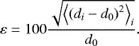
An example of initial conditions, including density perturbations constructed as described above, is presented in Fig. 1. We stress that unlike most of the previous dense core collapse studies, which attempted to form and study disks, we have no rotation or turbulence initially.
3.3 Choice of a time reference
Since the free-fall time depends on the density, it can slightly vary from a level of perturbation to another. As the grid is initially coarse, the first time-steps of the simulation are much larger than the ones just after the collapse occured, corresponding to a higher level of refinement. These two effects lead to a bad description in time at the beginning of the simulation. We were thus compelled to choose a time reference from which the ages were computed. We based our time reference on the maximum density inside the simulation box. For time reference, we used the moment when the maximum density reaches 10−13g cm−3. It corresponds to the limit density beyond which the compression of the dense gas changes from isothermal to adiabatic (Larson 1969).
 |
Fig. 1 Column density map along the y-axis of the simulation box, representing the initial conditions with a perturbation level of 50%. These perturbations in density are based on a Kolmogorov turbulent spectrum. Initially all of the velocities are set to zero so that the angular momentum in the box frame is initially null. |
4 Results
4.1 Formation of a disk
The main result of this study is, as we expected from our theoretical development, the formation of a disk within our simulations. We show a sequence of images of the disk growing with time in the simulation with 50% of density perturbations in Fig. 2. This disk is very similar to those found in many studies (Bate et al. 2003; Matsumoto & Hanawa 2003; Goodwin et al. 2004a; Hennebelle & Fromang 2008; Gray et al. 2018). As can be seen, it presents prominent spiral arms that transport angular momentum. To verify that this structure is a disk, we made sure to check that the structure that formed is rotationally supported. In order to keep our model as simple as possible, we did not use sink particles (Krumholz et al. 2004; Bleuler & Teyssier 2014) in our simulations that are presented in this section and analyzed in Sects. 4.2 and 4.3. As a consequence, the dense gas accumulates in the disk, making it self-gravitating. Thus, the azimuthal velocity profile shows substantial deviations from the Keplerian profile, but the structure is still rotationally supported, as the azimuthal velocity is much larger than the radial velocity inside the disk, typically by a factor of 50. However, we also show that disks form in simulations with sink particles (see Sect. 4.4) and we verified that the structures that formed match the Keplerian profile very well.
We ran a set of simulations that only differ by their perturbation level, from 10 to 60%. In all of these simulations, we observe the formation of a protostellar disk. The comparison with theory, which is studied in detail for the simulation with 50% of density perturbations in Sect. 4.2, gives clues to assess the trust level of our simulations; for the other levels of perturbation, the results are visible in Appendix B. For the simulations over 20% of perturbations, the comparison shows that the formation of the disk can be trusted. For the simulations with low perturbation level, which is typically less than 20%, the agreement with theory is not as good and the numerical errors are higher.
4.2 Comparison with theory
We show in Sect. 2.2 that a rotational structure should emerge from an asymmetric gravitational collapse, even without any initial motion. To compare this theoretical prediction with our simulations, we refer to Eqs. (3) and (4). The first expression simply expresses the numerical way to compute the total angular momentum in the simulation (in the frame  , with respect to the point C, what we will not mention anymore). We name this quantity σnum. The second one is the analytic expression of the same quantity. It is equivalent to the first one if a set of hypothesis is verified (see Appendix A.1), which is the case in our simulations. We refer to this quantity as σan. The equality of the two quantities σnum and σan ensures thatwe are observing the physical phenomenon we described. The differences could be due to numerical errors. Initially, we numerically verified the equality:
 (10)
(10)
The comparison between σnum and σan is represented on the top panel of Fig. 3 for the simulation with 50% of perturbations. The slight relative difference, which is roughly less than 2%, shows that the equality of these two quantities is numerically consistent. Furthermore, the relative difference does not maintain the same sign during the temporal evolution. It shows that this difference is not a systematic error for one of the two quantities.
We note . To be entirely surethat the disk that formed in our simulation is not a numerical artifact, we verified that the angular momentum it contains is larger than
  . In the most pessimistic scenario where
  would be entirely concentrated in the disk, this ensures that
  is not sufficient in explaining the presence of the disk. The angular momentum contained in the disk is computed as σnum, but in the restricted area of the simulation corresponding to the disk5. The comparison between
  and the angular momentum in the disk is visible on the bottom panel of Fig. 3. As
  is smaller than the angular momentum in the disk, and as Δσ switches signs over the temporal evolution of the system, it confirms that the formed disk is the result of the physics described in Sect. 2.2. For the other levels of perturbations, the results are presented in Appendix B.
4.3 Analysis of velocity gradients
In this section we analyze our simulations from an observational point of view to highlight whether or not our model succeeds in describing some features of real observations. Since the rotation emerges from the asymmetrical gravitational collapse in our model, it is not straightforwardly inherited from larger scales. This lack of connection between disk and envelope scales leads to important features. We computed three quantities at different scales that are accessible to observations: the direction and amplitude of velocity gradients and the specific angular momentum.
To compute the direction and amplitude of the velocity gradients at a scale R, we followed the method of Goodman et al. (1993). We considered a cube with a side of 2R around the disk, aligned with the three main axis of the simulation. We considered these three main axis as our lines of sight to compute maps of projected velocities that are weighted by density with a depth of 2R. Then we fit these maps with a solid-body rotation profile:
 (11)
(11)
in which v0 is the systemic velocity of our object and Δx and Δy are the vertical and horizontal dimensions of our map of projected velocities. The magnitude of the velocity gradient is thus  and its direction is given by
  . The specific angular momentum at a scale R is thus given by j = R2Ω.
In an axisymmetrical model with initial rotation, velocity gradients at small and large scales are perfectly aligned. In our model, due to the lack of initial rotation, it is interesting to see how velocity gradients at different scales are organized. The top panel of Fig. 4 shows the angular variation of velocity gradients according to the probed scale, relative to the velocity gradient at the disk scale. Velocity gradients in the disk and in the envelope are misaligned. For the y projection, the velocity gradient in the envelope is even reversed in comparison to the small scale gradient; whereas for the x projection, the velocity gradients make a complete turn from the disk to the envelope scales.
The amplitude of the velocity gradient at different scales is shown in the mid panel of Fig. 4. In the three projections, the amplitude profile from a hundred astronomical units roughly follows a power law of Ω ∝R−1.8. It shows that these gradients are detectable in real observations since the choice of appropriate molecular lines allows one to detect gradient amplitude about 1 km s−1 pc−1 in a solar type star-forming core at a distance of 200 pc.
Once we computed the amplitude of these gradients, we were able to determine the specific angular momentum. The evolution of this quantity at different scales is presented on the bottom panel of Fig. 4. This figure shows that for the three main lines of sight of the simulation, the specific angular momentum does not vary so much through the different scales, except for some peaks that correlate to abrupt changes in angular direction of velocity gradients. Furthermore, this quantity is roughly constant in the envelope, at the scale of a hundred and thousands of astronomical units, with a mean value of about 310−4 km s−1 pc. In the discussion section, we compare the projected kinematics properties of our modeled core to observations in protostellar envelopes.
To determine the origin of these velocity gradients, we computed the maps of projected velocities along the line of sight by only taking the radial part of the velocity into account with respect to the disk center, on the one hand, and the orthoradial part of the velocity on the other hand. We computed the velocity gradient directions over the differentscales for the radial and orthoradial part of the velocity as we did for the total velocity gradients. We compared the angular deviation between the total velocity gradient and the radial velocity gradient, Δθrad, and between the total velocity gradient and the orthoradial velocity gradient, Δθorthorad. The results for different levels of perturbation that were taken at similar times are visible in Fig. 5. For the simulation with 10% of perturbations, the total and radial velocity gradient directions are very close over the probed scales6. As the levelof perturbation increases, the radial and total gradients begin to misalign, and  increases, for scales larger than 400 AU; whereas the orthoradial and total gradient directions get closer, and
  decreases. These results depend on the line of sight chosen to compute the projected velocity, and to a lesser extent on the evolutionary stage of the simulations. What is a common feature is that for the small perturbation levels, the radial and total velocity gradient directions are very close over all of the probed scales.
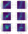 |
Fig. 2 Column density in the simulation with 50% of perturbations at three different times. Left: face-on projection. Right: edge-on projection. The rotation axis zd of the disk does not overlap with any simulation box axis. We see that a disk forms and grows in spite of the fact that the angular momentum is null initially. |
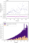 |
Fig. 3 Analysis of the simulation with 50% of perturbations. Top: σnum (see Eq. (3)) in blue, and the relative difference between σnum and σan (see Eq. (4)) in purple for each output. Bottom: momentum in the disk (in violet) compared to the absolute value of the difference between σnum and σan (in beige). We see that |

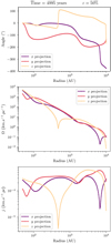 |
Fig. 4 Analysis of velocity gradients at different scales in the simulation with 50% of perturbations. In each panel, the three curves correspond to the three main projections of the simulation. Top: angular direction of velocity gradients. The origin of the angular direction corresponds to the direction of the disk scale gradient. Mid: amplitude of velocity gradients. Bottom: specific angular momentum as computed in analyses of observations. |
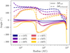 |
Fig. 5 Angle between radial and total velocity gradients (Δθrad, solid lines) and between orthoradial and total velocity gradients (Δθorthorad, dashed lines), for different levels of perturbation ε. For the simulation with 10 and 20% of perturbations, the total gradient directions follow the ones of the radial velocity gradients over all scales. For the simulations with more perturbations, Δθrad is higher for scales larger than 400 AU and Δθorthorad gets lower. |
4.4 Size of formed disks
We had not introduced any sink particle in our simulations until now. As a consequence, the gas cannot collapses at a smaller scale than our maximal resolution. This compels the gas to accumulate in the center of the disk; this causes the disk to become autogravitating and leads to the apparition of the spiral arms, which are visible in Fig. 2, to transport angular momentum inside the disk. As this accumulation of dense gas in the disk is not physical – the gas should continue to collapse to the stellar scales – it is not correct to compute the disk radius in these simulations. To handle this issue, we ran simulations with sink particles that were introduced when the density reaches the threshold of 1014 cm−3. The disk grows, but it is less massive than before, and it matches the Keplerian profile very well. At some point, the disk fragments. Figure 6 shows the disk at an advanced stage, shortly before fragmentation. The disk reaches a radius of about 125 AU, which is large in comparison to observed disk radii (Maury et al. 2010, 2019; Tobin et al. 2015; Segura-Cox et al. 2016). To compute the disk radius in our simulations, the first step was to isolate what belongs to the disk. This selection was based on density and velocity criterion: a cell has to be dense enough and the orthoradial component of its velocity has to be at least two times larger than the radial one. Once this selection was completed, we looked at the maximum distance projected inthe equatorial plane for a large number of angular sectors. The mean of these distances over the different angular sectors was taken as the disk radius. Figure 7 shows the evolution of the disk radius over time for several simulations. The three green curves show the radius of the disk in the simulations with a 10, 20, and 50% perturbation level. It appears that in these three simulations, the disks grow to reach radii around 200 AU in 20–30 kyr, before fragmenting. The disk size does not depend much on the perturbation level in the range of 10–50% of perturbations.
4.5 Effects of initial rotation
To see the influence of initial rotation on our results, we ran four simulations in which a solid-body rotation velocity profile is imprinted in the initial conditions. We ran simulations with ε = 20 and 50%, and for each of these perturbation levels, we chose two rotation levels7 β =0.25 and 1%. The evolution of the disk radius in these simulations is visible in Fig. 7, which is represented by the four curves from red to yellow. For these four simulations, the evolution of the radius is similar. These disk grows rapidly before fragmenting between 2 and 7 kyr at a radius around 100 AU. This evolution is different from those of the disks in the simulation without initial rotation, in particular, because the disk forms earlier and grows faster. Whereas, when there is no rotation, it takes about 15 kyr to get a disk that is bigger than 100 AU; this only takes 3–5 kyr when rotation is included.
In these simulations, we conducted the same analysis of velocity gradients as in Sect. 4.3. The results for the simulation with ε = 50% and β =1% are shown in Figs. 8 and 9. In the top panel of Fig. 8, we see that the angular deviations of the velocity gradients are less pronounced than in the case without initial rotation. Only the face-on projection exhibits large deviations, but the amplitude Ω in this projection is much smaller than in the two edge-on projections by a factor of around 10. The resulting specific angular momentum is visible in the bottom panel of Fig. 8. For the two edge-on projections, it exhibits values that are larger than in the case without initial rotation and also those that were deduced from observations. We also see that j ∝ Rα with α ≃ 0.5 while observations revealed that in the inner few thousands of astronomical units, α ≃0 (see Belloche 2013 for a review). The most recent observations by Gaudel et al. (2020) reveal α ≃0.3 ± 0.3 under 1600 AU.
Here, we also computed the decomposition of the velocity in its radial and orthoradial components and conducted the same analysis of velocity gradients with these two components. The results are visible in Fig. 9 for the full velocity gradients, the radial velocity gradients, and orthoradial velocity gradients in the simulation with ε = 50% and β = 1% for the edge-on projection 1. The top panel shows the angle using the same arbitrary reference for the three gradients, whereas the middle and bottom panels show the amplitude and the specific angular momentum deduced from these gradients, respectively. The joint analysis of the top and middle panel shows that for R < 102 AU and R > 3 × 10³ AU, the orthoradial velocity gradient is dominant since it is much larger in amplitude than the radial one and it is much closer to the full velocity gradient in angular position than the radial one is. This means that at a large scale, the full velocity gradient traces the rotation of the envelope. For 102 AU < R < 3 × 10³ AU, the contribution of the radial and orhoradial component are of the same order of magnitude in amplitude, which leads to the full velocity gradients to be misaligned with both the radial and orthoradial gradients at those scales. In the face-on projection, the effect of the rotation is nearly invisible and the results are similar to the ones presented Sect. 4.3. The results are comparable for the four simulations introduced in this section and, therefore, the other cases are not shown for conciseness.
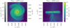 |
Fig. 6 Column density in the simulation with 50% of perturbations and with sink particle (red circle). Left: face-on projection. Right: edge-on projection. At this time, the sink particle has a mass of 0.64 M⊙. The disk is large with a radius of nearly 125 AU. |
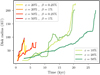 |
Fig. 7 Temporal evolution of disk size for a set of simulations. The three green curves are purely hydrodynamics simulations with different levels of perturbations ε. The four curves from red to yellow are also purely hydrodynamics, but they include an initial solid-body rotation velocity profile, with different levels of perturbations and rotation β. The curves stop when the disk fragments. All of the plotted curves were smoothed by a sliding median. |
4.6 Effects of the magnetic field
For the sake of completeness, we finally added a magnetic field8 in our simulations to see its effects on the formed disk. The magnetic field is treated under the ideal MHD approximation. In these simulations, a disk still forms even in the absence of initial large scale rotation. Figure 10 shows the appearance of the disk at the same time as in Fig. 6. Clearly the two disks are qualitatively very different. In the purely hydrodynamics case, the disk is big and massive, with sharp edges, whereas in the MHD case, the disk is smaller and less massive (smaller column density).
In the MHD case, it is hard to define a disk’s radius properly. In fact, when looking at Fig. 10, the disk is buried in a very filamentary structure that has the same order of magnitude in column density as the outer part of the disk. At some places these filaments verify the velocity criteria set out in Sect. 4.4 to define the belonging to the disk. Here, we are confronted with a definition problem. In hydrodynamics simulations, the disk has sharp edges and it is clear as to what belongs to the disk or not by the naked eye. In MHD simulations, it is really hard to do so and, therefore, we do not attempt to present a quantitative comparison here.
In spite of this difficulty, the comparison between Figs. 6 and 10 reveals that in the MHD case, the disk is much smaller. For the MHD simulation without initial rotation, the disk stops growing after 20 kyr and does not fragment like in the hydrodynamics case. For the simulation with initial rotation, the disk grows more rapidly but it also stabilizes at the same size between 40 to 70 AU depending on the definition of what belongs to the disk. We believe that this is the signature of the magnetic braking that occurs in magnetized disk.
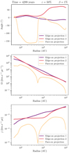 |
Fig. 8 Analysis of velocity gradients at different scales in the simulation with 50% of perturbations and β = 1%. On each panel, the three curves correspond to two edge-on and one face-on projections. Top: angular direction of velocity gradients. The origin of the angular direction corresponds to the direction of the disk scale gradient. Middle: amplitude of velocity gradients. Bottom: specific angular momentum as computed in observation analysis. |
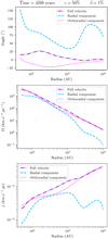 |
Fig. 9 Analysis of velocity gradients for the full velocity (in purple dashdotted), the radial component (in blue dashed), and the orthoradial component (pink dotted). These quantities are represented at different scales in the simulation with 50% of perturbations and β = 1%, for the edge-on projection 1. Top: angular direction of velocity gradients. The origin of the angular direction corresponds to the direction of the disk scale gradient. Middle: amplitude of velocity gradients. Bottom: specific angular momentum as computed in observation analysis. |
5 Discussion
From a very simple model, we show that the angular momentum computed in the frame of the disk in relation to the center of the disk is not a conserved quantity. This is due to the non-Galilean nature of the frame, which is provoked by the nonaxisymmetrical gravitational collapse. This collapse leads to the formation of a protostellar disk. In our system, the angular momentum that forms the disk is not a mere conservation of preexisting large scale angular momentum. The rotation can be generated locally by the asymmetry of the collapse. This result is in agreement with the early work by Peebles (1969). This mechanism, which is responsible for the formation of spiral galaxies, is thus also able to account for the formation of protostellar disks. Thereby, the conservation of a preexisting angular momentum at large scales might not be the only mechanism responsible for protostellar disk formation, and the assumption that small scale rotation is being inherited from the large scales may not be correct, at least for some systems.
The disks that formed in the simulations with sink particles reach a radius that is larger than a hundred astronomical units until they fragment. As these simulations start with no angular momentum and only require moderate density perturbations, which are expected to be present in real cores, this study gives a sort of “minimal hydrodynamic radius” that a disk should reach in a hydrodynamics collapse. As most of the observed disks are much smaller (Maury et al. 2010, 2019; Tobin et al. 2015; Segura-Cox et al. 2016), this implies that angular momentum extraction processes are at work in real disks. In the traditional picture of axisymmetric collapse, the size of the disk directly depends on the initial rotation. The presence of small disks in observations could therefore be interpreted as being due to low rotation levels. In the present study, we show that in the nonaxisymmetric case, even modest levels of density perturbations lead to the formation of large disks that have a size of about a hundred astronomical units. The latter appears to be the natural outcome of the gravitational dynamics and local conservation of angular momentum. These disks are thus generic features. Therefore, the most natural way to reconcile these observations with the generic nature of big hydrodynamical disks is to invoke the presence of magnetic braking, which we know is operating in cores (Li et al. 2014; Hennebelle & Inutsuka 2019). Our MHD simulation starting from the same initial conditions but just adding a magnetic field shows that the outcoming disk is much smaller and it does not fragment, which is as expected from these previous studies.
The magnitudes of the velocity gradients from our modeled core do not depend much on the chosen projection, although a dip is observed in the z projection at scales of 600 AU (see mid panel of Fig. 4), which is the result of a reversal in angular direction of velocity gradients. Their amplitude is roughly consistent with velocity gradients observed in protostellar cores using dense gas tracers (see, for example, Chen et al. 2007; Belloche & André 2004 who recover amplitudes from 0.1 to 10 km s−1 pc−1 in protostellar cores at scales of 5000 AU) and also with the recent results of Gaudel et al. (2020) who probe inner regions of Class 0 envelopes down to a hundred astronomical units. The specific angular momentum j in our modeled core, which was computed from the velocity gradients following a similar methodology as the one extracting j from observations, has a roughly constant value of about 3 × 10⁻⁴ km s−1 pc between 102 and 103 AU (see bottom panel of Fig. 4). This order of magnitude is similar to typical specific angular momentum values recovered from observations in solar-type protostellar cores: see Yen et al. (2015a) for observations in seven Class 0 protostars and the work of Gaudel et al. (2020) in 12 Class 0 protostars that give a specific angular momentum of 5 × 10⁻⁴ km s−1 pc below 1400 AU. The few observational constraints on the spatial distribution of specific angular momentum in prestellar cores and protostars suggest a scenario where local specific angular momentum follows a power-law R1.6 in starless structures at scales larger than 6000 AU, while it is constant and conserved within collapsing star-forming cores (see Belloche 2013 for a review). However, Yen et al. (2015b) find that the decreasing trend of j(R) observed at large scales propagates down to radii that are smaller than 5000 AU. Gaudel et al. (2020) resolved the break radius around 1600 AU where it stabilizes with a weak dependence on radius j ∝ R0.3±0.3 between 50 and 1600 AU. These observations are very well matched by the properties of specific angular momentum in our simulations with density perturbations and no rotation. Our model shows a dependency of Ω along a R−1.8 power-law, which translates9 to a j ∝ R0.2 power-law that is centered on the value of 3 × 10⁻⁴ km s−1 pc, coinciding with the recent observational results cited earlier.
However, the analysis of velocity gradients also reveals a large dispersion of the gradient directions between the disk and envelope scales. Depending on the viewing angle, the observed velocity gradients in the envelope can be very misaligned with respect to the small-scale gradient resulting from disk rotation. The projected kinematics can even produce a complete reversal of the gradient at some scales. For example in the top panel of Fig. 4, the y projection (red curve) shows a gradient about 200 ° from the disk scale gradient at scales of 2000 AU. Since the rotation is generated locally in our model, it is not surprising that small and large scale gradients are unrelated and hence misaligned. In our model, there is no large scale rotation, suggesting that observations of strongly misaligned gradients in protostellar cores could be due to nonaxisymmetric gravitational collapse, rather than to global rotational motions of the core. Such a scenario could explain, for example, the reversal of velocity gradients observed in the L1527 protostar (Tobin et al. 2011) or our recent findings that the rotation of the small-scale disk in the low-luminosity protostar IRAM 04191 (Maury et al., in prep.) is opposite to the large-scale gradient at 2000 AU scales in the envelope, which is interpreted as core rotation (Belloche & André 2004). This observation of a “counter-rotating” disk is incompatible with simple axisymmetrical collapse models in which the disk would have simply formed because of the conservation of a large scale angular momentum in a rotating core. Tsukamoto et al. (2017) developed MHD models, including the Hall effect, that form counter-rotating envelopes at the upper region of a pseudo-disk under some conditions about the alignment between the magnetic field and initial rotation. This thin counter-rotating layer is located close to the pseudo-disk, typically between 50 and 200 AU, and they are thus unable to explain counter-rotation in the outer envelopes, at scales larger than 1000 AU, while it is a natural feature of our model.
The analysis of the radial and orthoradial part of the velocity and their contribution to the total velocity gradient directions shows that for small perturbation levels (typically less than 20%), the radial and total velocity gradient directions are very close over all of the probed scales, whereas the orthoradial component is misaligned. As the perturbation level increases, for scales larger than 400 AU the radial component is more and more misaligned; whereas the orthoradial one tends to be closer to the total velocity gradient direction. These features depend on the choice of the line of sight. A common point, which seems independent from the choice of a line of sight, is that for small perturbation levels, the radial component is very close to the total velocity gradient direction. Since the simulations start with no global rotation, this analysis shows that the notion of radial and orthoradial though as infall and rotation is less and less clear as the level of perturbations increases, which means as the deviation from axisymmetry grows. With a small perturbation level, the deviation from axisymmetry is low and the velocity gradients are mainly due to infall motions. With large perturbation levels, the deviation from axisymmetry is high and the velocity gradients result from the complex dynamics of the self- gravitating gas.
When adding global rotation to the initial conditions, we found that the formed disks grow more rapidly and fragment earlier. In analyzing the kinematics of the gas in those simulations with initial rotation, we show that the angular deviations are lower than in the case without initial rotation, which is less in agreement with the observational results from Gaudel et al. (2020). From this analysis, the inferred specific angular momentum exhibits a slope and a mean value larger than in the case without initial rotation. As for the angular deviation, this result is in agreement to a lesser extent with observations than in the case without initial rotation.
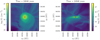 |
Fig. 10 Column density in the MHD simulation with 50% of perturbations and with sink particle (red circle), at the same time than Fig. 6. Left: face-on projection. Right: edge-on projection. At this time, the sink particle has a mass of 0.40 M⊙. It is hard todefine a proper disk radius in this case. |
6 Conclusion
We show that protostellar disks can emerge from a nonaxisymmetrical gravitational collapse in which there is no rotation initially. We ran purely hydrodynamical simulations of a collapsing dense core starting from an initial condition where all the cells are at rest, and we broke the symmetry of the problem by adding density fluctuations over a flat profile. We show analytically that the angular momentum in the frame of the accretion center and with respect to the accretion center is not a conserved quantity due to the non-Galilean character of the frame. This leads to the possibility of the formation of a disk and we demonstrate numerically that a disk indeed forms in these simulations.
We then analyze our simulations from an observational point of view by computing the velocity gradients at different scales, as is done with real observations, and by deducing the amplitude of these gradients and the specific angular momentum over the different scales. The results we obtained for the value of the specific angular momentum matches the ones from Belloche (2013) and Gaudel et al. (2020).
This study then suggests a new paradigm as to the formation of protostellar disks, but it does not replace the current one regarding the conservation of preexisting angular momentum at a large scale. It shows that even if this conservation of angular momentum is absolutely correct in an axisymmetrical model, it is more complicated when the axisymmetry is broken since the accretion center frame becomes non-Galilean. In the extreme case we studied in which every cell is initially at rest, it shows that even without initial rotation, the formation of a protostellar disk is possible. The formation of these disks in our model no longer depends on the specificities of large scales, but it results in a more generic process that is only due to the density fluctuations of the gas. We show that the different features of the model based on the analysis of velocity gradients are realistic. This model could thus help in understanding the features observed in some objects as the angular deviation of velocity gradients at different scales. It also helps in understanding the formation of a disk within progenitors, which do not seem to contain enough angular momentum at large scales to form a disk by conservation of the angular momentum during the collapse. We find that these models without initial rotation are in better agreement with observational results than the models with initial solid-body rotation.
Our model uses the following minimal physical ingredients: hydrodynamics, thermodynamics, gravity, and density fluctuations. It is thus robust in the sense that all of these ingredients are always present in dense cores. In particular, we find that a disk forms even for density perturbations as low as 10%. Protostellar disks appear to be natural features of a gravitational collapse as soon as it is not axisymmetric. Since large disks are formed in this new scenario, we stress the necessity to evoke processes extracting angular momentum to lead to the formation of smaller disks, as found with observations. We show that the presence of a magnetic field reducesthe size of the formed disk, which is in agreement with past studies (Hennebelle et al. 2016; Maury et al. 2018).
Acknowledgements
We sincerely acknowledge the anonymous referee for the revision of our work and for the comments and suggestions.
Appendix A Full theoretical development
A.1 Development from the angular momentum in the box frame
In this annex, we reused the notations and definitions found in Sect. 2.2. The frame  of the simulation box is Galilean and there are not any external forces that are applied on the system of material points. The angular momentum
  that is computed in
 in relation to O is thus conserved. For the entire development, we consider an initial condition where all of the points are motionless in
  , this ensure that
  is equal to zero and that it stays null through the temporal evolution of the system.
 (A.1)
(A.1)
From this expression, we can include the accretion center C:
 (A.2)
(A.2)
By involvingthe expression of the total mass  , by using the definition of the center of mass G that implies
 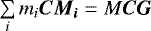 , and by recognising10 that the fourth term of the expression above if the angular moment
  defined Eq. (3), we obtain:
 (A.3)
(A.3)
By rewritingthe second term, the point G appears as follows:
 (A.4)
(A.4)
In reuniting the first term with the fourth one, and then with the second one, we obtain:
 (A.5)
(A.5)
We can apply the inertia center theorem to the whole system of material points in  . In the lack of external force, it gives:
![Mathematical equation: \[ M \frac{\, \mathrm{d} ^2 \bm{OG}}{\, \mathrm{d} t^2} = \bm{F_{\text{ext}}} = \bm{0} ~~~\Longrightarrow ~~~ \frac{\, \mathrm{d} \bm{OG}}{\, \mathrm{d} t} = \bm{\text{cte}} = \bm{0} \]](/articles/aa/full_html/2020/03/aa36394-19/aa36394-19-eq63.png)
because the velocity in each point is initially null. Then only two terms remain in the Eq. (A.5), which can be rewritten in the form of the Eq. (4):
 (A.6)
(A.6)
This expression is equivalent to  due to the fact that
  .
.
A.2 Interpretation with the inertial force
We consider the problem from the frame  . The latter is not Galilean, and we chose it to be in translation with respect to
  , without loosing any generality, in order to have the equality of the temporal derivative operators in
  and
and  . We can thus rewrite the evolution equation of the angular momentum
  in the absence of external forces:
 (A.7)
(A.7)
where  is the torque of the inertial force that is exerted on each point i, in relation to the point C. For the given conditions of
  , this force can be written as:
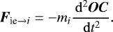 (A.8)
(A.8)
We can thus write the momentum of Fie→i in relation to the point C as:
 (A.9)
(A.9)
By reusing the definition of the center of mass and the fact that  , the right side of Eq. (A.7) becomes:
 (A.10)
Equation (A.7) then becomes :
 (A.11)
This expression is the same as the one obtained by taking the derivative of Eq. (A.6), but it allows us to understand that the nonconservation of the angular momentum is due to the non-Galilean character of the frame
 .
.
Appendix B Numerical validity
In this annex, we reuse the notations found in Sect. 4.2. We show in Sect. 4.2 that in looking at the difference between σnum and σan and in comparing this difference to the momentum in the disk, this gives us a simple way to estimate the trust level of our simulations. The results for all of the perturbation levels we studied are given in Fig. B.1. The left panel shows the relative difference between σnum and σan. Except for the simulation with ε = 10%, this difference is less than a few percent. For the simulation with 10% of perturbation, this difference grows higher.
In order to conclude on the trust level on the simulations, we have to compare to the angular momentum  contained inthe disk. This relative comparison is visible in the right panel of Fig. B.1. A value close to 1 means that Δσ is negligible compared to the momentum in the disk. A value of 0 or lower means that
  is equal or higher than
  . In this latter case, we cannot exclude the worst scenario where all of the numerical errors would be concentrated at the same location, resulting in the formation of a disk that is then a numerical artifact. The right panel of Fig. B.1 shows the results until the disk starts to fragment since our disk isolation algorithm gives correct results only when a single disk is present in the simulation box. These results show that the simulation with ε = 50% is the best in terms of trust level. For the other levels of perturbation, the trust level is lower, but as this relative difference remains higher than 0.1, even the worst scenario cannot explain the amount of angular momentum present in the disk in terms of numerical errors.
 |
Fig. B.1 Analysis of numerical errors in the simulations with different levels of perturbations ε, without sinkparticle. The legend is the same for both panels. To improve visibility, the results have been smoothed. Left: relative difference between σnum and σan. Right: relative difference between the momentum in the disk |


References
- Bate, M. R. 1998, ApJ, 508, L95 [NASA ADS] [CrossRef] [Google Scholar]
- Bate, M. R., Bonnell, I. A., & Bromm, V. 2003, MNRAS, 339, 577 [NASA ADS] [CrossRef] [Google Scholar]
- Belloche, A. 2013, EAS Pub. Ser., 62, 25 [CrossRef] [EDP Sciences] [Google Scholar]
- Belloche, A., & André, P. 2004, A&A, 419, L35 [NASA ADS] [CrossRef] [EDP Sciences] [Google Scholar]
- Bleuler, A., & Teyssier, R. 2014, MNRAS, 445, 4015 [NASA ADS] [CrossRef] [Google Scholar]
- Chen, X., Launhardt, R., & Henning, T. 2007, ApJ, 669, 1058 [NASA ADS] [CrossRef] [Google Scholar]
- Dib, S., Hennebelle, P., Pineda, J. E., et al. 2010, ApJ, 723, 425 [NASA ADS] [CrossRef] [Google Scholar]
- Dutrey, A., Semenov, D., Chapillon, E., et al. 2014, Protostars and Planets VI (Tucson, AZ: University of Arizona Press), 317 [Google Scholar]
- Gaudel, M., Maury, A. J., Belloche, A., et al. 2020, A&A, in press, https://doi.org/10.1051/0004-6361/201936364 [Google Scholar]
- Goodman, A. A., Benson, P. J., Fuller, G. A., & Myers, P. C. 1993, ApJ, 406, 528 [NASA ADS] [CrossRef] [Google Scholar]
- Goodwin, S. P., Whitworth, A. P., & Ward-Thompson, D. 2004a, A&A, 414, 633 [Google Scholar]
- Goodwin, S. P., Whitworth, A. P., & Ward-Thompson, D. 2004b, A&A, 423, 169 [NASA ADS] [CrossRef] [EDP Sciences] [Google Scholar]
- Gray, W. J., McKee, C. F., & Klein, R. I. 2018, MNRAS, 473, 2124 [NASA ADS] [CrossRef] [Google Scholar]
- Harsono, D., Jørgensen, J. K., van Dishoeck, E. F., et al. 2014, A&A, 562, A77 [NASA ADS] [CrossRef] [EDP Sciences] [Google Scholar]
- Hennebelle, P., & Falgarone, E. 2012, A&ARv, 20, 55 [NASA ADS] [CrossRef] [Google Scholar]
- Hennebelle, P., & Fromang, S. 2008, A&A, 477, 9 [NASA ADS] [CrossRef] [EDP Sciences] [Google Scholar]
- Hennebelle, P., & Inutsuka, S.-i. 2019, Front. Astron. Space Sci., 6, 5 [NASA ADS] [CrossRef] [Google Scholar]
- Hennebelle, P., Commerçon, B., Chabrier, G., & Marchand, P. 2016, ApJ, 830, L8 [NASA ADS] [CrossRef] [Google Scholar]
- Hoyle, F. 1949, MNRAS, 109, 365 [Google Scholar]
- Krumholz, M. R., McKee, C. F., & Klein, R. I. 2004, ApJ, 611, 399 [NASA ADS] [CrossRef] [Google Scholar]
- Kurtovic, N. T., Pérez, L. M., Benisty, M., et al. 2018, ApJ, 869, L44 [Google Scholar]
- Kuznetsova, A., Hartmann, L., & Heitsch, F. 2019, ApJ, 876, 33 [NASA ADS] [CrossRef] [Google Scholar]
- Larson, R. B. 1969, MNRAS, 145, 271 [NASA ADS] [CrossRef] [Google Scholar]
- Li, Z.-Y., Banerjee, R., Pudritz, R. E., et al. 2014, Protostars and Planets VI (Tucson, AZ: University of Arizona Press), 173 [Google Scholar]
- Machida, M. N., Matsumoto, T., Tomisaka, K., & Hanawa, T. 2005, MNRAS, 362, 369 [NASA ADS] [CrossRef] [Google Scholar]
- Matsumoto, T., & Hanawa, T. 2003, ApJ, 595, 913 [NASA ADS] [CrossRef] [Google Scholar]
- Matsumoto, T., Machida, M. N., & Inutsuka, S.-i. 2017, ApJ, 839, 69 [NASA ADS] [CrossRef] [Google Scholar]
- Maury, A. J., André, P., Hennebelle, P., et al. 2010, A&A, 512, A40 [NASA ADS] [CrossRef] [EDP Sciences] [Google Scholar]
- Maury, A. J., Girart, J. M., Zhang, Q., et al. 2018, MNRAS, 477, 2760 [Google Scholar]
- Maury, A. J., André, P., Testi, L., et al. 2019, A&A, 621, A76 [NASA ADS] [CrossRef] [EDP Sciences] [Google Scholar]
- Ohashi, N., Hayashi, M., Ho, P. T. P., et al. 1997, ApJ, 488, 317 [NASA ADS] [CrossRef] [Google Scholar]
- Peebles, P. J. E. 1969, ApJ, 155, 393 [NASA ADS] [CrossRef] [Google Scholar]
- Pérez, L. M., Benisty, M., Andrews, S. M., et al. 2018, ApJ, 869, L50 [NASA ADS] [CrossRef] [Google Scholar]
- Pineda, J. E., Zhao, B., Schmiedeke, A., et al. 2019, ApJ, 882, 103 [NASA ADS] [CrossRef] [EDP Sciences] [Google Scholar]
- Sciama, D. W. 1955, MNRAS, 115, 3 [Google Scholar]
- Segura-Cox, D. M., Harris, R. J., Tobin, J. J., et al. 2016, ApJ, 817, L14 [NASA ADS] [CrossRef] [Google Scholar]
- Simon, M., Dutrey, A., & Guilloteau, S. 2000, ApJ, 545, 1034 [NASA ADS] [CrossRef] [Google Scholar]
- Takakuwa, S., Tsukamoto, Y., Saigo, K., & Saito, M. 2018, ApJ, 865, 51 [NASA ADS] [CrossRef] [Google Scholar]
- Testi, L., Birnstiel, T., Ricci, L., et al. 2014, Protostars and Planets VI (Tucson, AZ: University of Arizona Press), 339 [Google Scholar]
- Teyssier, R. 2002, A&A, 385, 337 [NASA ADS] [CrossRef] [EDP Sciences] [Google Scholar]
- Tobin, J. J., Hartmann, L., Bergin, E., et al. 2011, IAU Symp., 270, 49 [NASA ADS] [Google Scholar]
- Tobin, J. J., Looney, L. W., Wilner, D. J., et al. 2015, ApJ, 805, 125 [NASA ADS] [CrossRef] [Google Scholar]
- Tobin, J. J., Bos, S. P., Dunham, M. M., Bourke, T. L., & van der Marel, N. 2018, ApJ, 856, 164 [NASA ADS] [CrossRef] [Google Scholar]
- Tsukamoto, Y., Okuzumi, S., Iwasaki, K., Machida, M. N., & Inutsuka, S.-i. 2017, PASJ, 69, 95 [CrossRef] [Google Scholar]
- Yen, H.-W., Koch, P. M., Takakuwa, S., et al. 2015a, ApJ, 799, 193 [NASA ADS] [CrossRef] [Google Scholar]
- Yen, H.-W., Takakuwa, S., Koch, P. M., et al. 2015b, ApJ, 812, 129 [NASA ADS] [CrossRef] [Google Scholar]
In fact, in relation to any fixed point of the simulation.
The center of mass remains motionless in the frame  of the simulation box due to the lack of external force. See Appendix A.1 for more details.
 .
.
The operation is simply :  with be
and af
referring to before and after the renormalization operation, which naturally leads to
with be
and af
referring to before and after the renormalization operation, which naturally leads to
 .
.
To belong to the disk, we consider that a cell has to have a high enough density and an azimuthal velocity that is larger than twice the radial velocity.
The smallest scale probed is 50 AU, which is a bit more than the disk radius at the moment the gradients were computed.
β is the ratio of rotational over gravitational energy.
We set a magnetization of μ = 0.3. For the MHD simulation with initial rotation, the axis of the magnetic field and the axis of rotation are aligned.
We note that j = R2Ω.
We chose  to be in translation with respect to
  in order to have the equality of the temporal derivative operators in the two frames, without loosing any generality.
All Figures
|
Fig. 1 Column density map along the y-axis of the simulation box, representing the initial conditions with a perturbation level of 50%. These perturbations in density are based on a Kolmogorov turbulent spectrum. Initially all of the velocities are set to zero so that the angular momentum in the box frame is initially null. |
| In the text | |
|
Fig. 2 Column density in the simulation with 50% of perturbations at three different times. Left: face-on projection. Right: edge-on projection. The rotation axis zd of the disk does not overlap with any simulation box axis. We see that a disk forms and grows in spite of the fact that the angular momentum is null initially. |
| In the text | |
|
Fig. 3 Analysis of the simulation with 50% of perturbations. Top: σnum (see Eq. (3)) in blue, and the relative difference between σnum and σan (see Eq. (4)) in purple for each output. Bottom: momentum in the disk (in violet) compared to the absolute value of the difference between σnum and σan (in beige). We see that |
| In the text | |
|
Fig. 4 Analysis of velocity gradients at different scales in the simulation with 50% of perturbations. In each panel, the three curves correspond to the three main projections of the simulation. Top: angular direction of velocity gradients. The origin of the angular direction corresponds to the direction of the disk scale gradient. Mid: amplitude of velocity gradients. Bottom: specific angular momentum as computed in analyses of observations. |
| In the text | |
|
Fig. 5 Angle between radial and total velocity gradients (Δθrad, solid lines) and between orthoradial and total velocity gradients (Δθorthorad, dashed lines), for different levels of perturbation ε. For the simulation with 10 and 20% of perturbations, the total gradient directions follow the ones of the radial velocity gradients over all scales. For the simulations with more perturbations, Δθrad is higher for scales larger than 400 AU and Δθorthorad gets lower. |
| In the text | |
|
Fig. 6 Column density in the simulation with 50% of perturbations and with sink particle (red circle). Left: face-on projection. Right: edge-on projection. At this time, the sink particle has a mass of 0.64 M⊙. The disk is large with a radius of nearly 125 AU. |
| In the text | |
|
Fig. 7 Temporal evolution of disk size for a set of simulations. The three green curves are purely hydrodynamics simulations with different levels of perturbations ε. The four curves from red to yellow are also purely hydrodynamics, but they include an initial solid-body rotation velocity profile, with different levels of perturbations and rotation β. The curves stop when the disk fragments. All of the plotted curves were smoothed by a sliding median. |
| In the text | |
|
Fig. 8 Analysis of velocity gradients at different scales in the simulation with 50% of perturbations and β = 1%. On each panel, the three curves correspond to two edge-on and one face-on projections. Top: angular direction of velocity gradients. The origin of the angular direction corresponds to the direction of the disk scale gradient. Middle: amplitude of velocity gradients. Bottom: specific angular momentum as computed in observation analysis. |
| In the text | |
|
Fig. 9 Analysis of velocity gradients for the full velocity (in purple dashdotted), the radial component (in blue dashed), and the orthoradial component (pink dotted). These quantities are represented at different scales in the simulation with 50% of perturbations and β = 1%, for the edge-on projection 1. Top: angular direction of velocity gradients. The origin of the angular direction corresponds to the direction of the disk scale gradient. Middle: amplitude of velocity gradients. Bottom: specific angular momentum as computed in observation analysis. |
| In the text | |
|
Fig. 10 Column density in the MHD simulation with 50% of perturbations and with sink particle (red circle), at the same time than Fig. 6. Left: face-on projection. Right: edge-on projection. At this time, the sink particle has a mass of 0.40 M⊙. It is hard todefine a proper disk radius in this case. |
| In the text | |
|
Fig. B.1 Analysis of numerical errors in the simulations with different levels of perturbations ε, without sinkparticle. The legend is the same for both panels. To improve visibility, the results have been smoothed. Left: relative difference between σnum and σan. Right: relative difference between the momentum in the disk |
| In the text | |
Current usage metrics show cumulative count of Article Views (full-text article views including HTML views, PDF and ePub downloads, according to the available data) and Abstracts Views on Vision4Press platform.
Data correspond to usage on the plateform after 2015. The current usage metrics is available 48-96 hours after online publication and is updated daily on week days.
Initial download of the metrics may take a while.