| Issue |
A&A
Volume 656, December 2021
|
|
|---|---|---|
| Article Number | A85 | |
| Number of page(s) | 19 | |
| Section | Interstellar and circumstellar matter | |
| DOI | https://doi.org/10.1051/0004-6361/202141648 | |
| Published online | 07 December 2021 | |
Collapse of turbulent massive cores with ambipolar diffusion and hybrid radiative transfer
II. Outflows
1
AIM, CEA, CNRS, Université Paris-Saclay, Université de Paris,
91191
Gif-sur-Yvette,
France
e-mail: This email address is being protected from spambots. You need JavaScript enabled to view it.
2
Université de Paris, CNRS, Astroparticule et Cosmologie,
75013
Paris,
France
3
Centre de Recherche Astrophysique de Lyon UMR5574, ENS de Lyon, Univ. Lyon1, CNRS, Université de Lyon,
69007
Lyon,
France
Received:
27
June
2021
Accepted:
10
September
2021
Abstract
Context. Most massive protostars exhibit bipolar outflows. Nonetheless, there is no consensus regarding the mechanism at the origin of these outflows, nor on the cause of the less-frequently observed monopolar outflows.
Aims. We aim to identify the origin of early massive protostellar outflows, focusing on the combined effects of radiative transfer and magnetic fields in a turbulent medium.
Methods. We use four state-of-the-art radiation-magnetohydrodynamical simulations following the collapse of massive 100 M⊙ pre-stellar cores with the RAMSES code. Turbulence is taken into account via initial velocity dispersion. We use a hybrid radiative transfer method and include ambipolar diffusion.
Results. Turbulence delays the launching of outflows, which appear to be mainly driven by magnetohydrodynamical processes. We study both the magnetic tower flow and the magneto-centrifugal acceleration as possible origins. Both contribute to the acceleration and the former operates on larger volumes than the latter. Our finest resolution, 5 AU, does not allow us to get converged results on magneto-centrifugally accelerated outflows. Radiative acceleration takes place as well, dominates in the star vicinity, enlarges the outflow extent, and has no negative impact on the launching of magnetic outflows (up to M ~17 M⊙, L ~ 105 L⊙). We observe mass outflow rates of 10−5−10−4 M⊙ yr−1 and momentum rates of the order ~10−4 M⊙ km s−1 yr−1. The associated opening angles (20−30deg when magnetic fields dominate) are in a range between observed values for wide-angle outflows and collimated outflows. If confirmed with a finer numerical resolution at the outflow interface, this suggests additional (de-)collimating effects. Outflows are launched nearly perpendicular to the disk and are misaligned with the initial core-scale magnetic fields, in agreement with several observational studies. In the most turbulent run, the outflow is monopolar.
Conclusions. Magnetic processes are dominant over radiative ones in the acceleration of massive protostellar outflows of up to ~17 M⊙. Turbulence perturbs the outflow launching and is a possible explanation for monopolar outflows.
Key words: stars: formation / stars: massive / stars: protostars / radiative transfer / magnetohydrodynamics (MHD) / methods: numerical
© R. Mignon-Risse et al. 2021
 Open Access article, published by EDP Sciences, under the terms of the Creative Commons Attribution License (https://creativecommons.org/licenses/by/4.0), which permits unrestricted use, distribution, and reproduction in any medium, provided the original work is properly cited.
1 Introduction
Massive stars form in dense environments, and one of their birth signs is the presence of (often bipolar) outflows. Nevertheless, their large luminosities, together with the presence of magnetic fields in their birth place, has complicated the task of understanding the origin of these outflows. Indeed, while it is now quite well accepted that low-mass protostars power magnetically driven outflows (see e.g., Pudritz & Ray 2019 and references therein), the strong radiative force from massive protostars is also capable of launching outflows (Krumholz & Matzner 2009; Kuiper et al. 2011; Rosen et al. 2016; Mignon-Risse et al. 2020). Moreover, magnetic protostellar outflows rely on disk-mediated accretion, while the accretion mechanism of massive protostars has long been debated, with additional modes such as accretion via stellar collisions (Bonnell et al. 1998); radiative Rayleigh-Taylor instabilities (Krumholz & Matzner 2009; Rosen et al. 2016), or dense filaments (Rosen et al. 2016). Distinguishing between a magnetically driven and a radiatively driven outflow in a self-consistent way requires, at the very least, solving the magnetohydrodynamics (MHD) equations coupled to radiative transfer equations. This is the purpose of the present paper.
There are now numerous observational clues as to the outflow mechanism around massive protostars. Several works agree on a clear correlation between the source radio luminosity up to 105 L⊙, the core mass, and the outflow momentum rate (Anglada et al. 1992; Cabrit & Bertout 1992; Beuther et al. 2002, see the review by Anglada et al. 2018). This correlation is found to continue to high luminosities, that is, for high-mass protostars (core masses ranging from hundreds to thousands of solar masses, Beuther et al. 2002). Collimated jets, a common feature of low-mass star formation are also observed around massive young-stellar objects (e.g., Moscadelli et al. 2005). As there is no clear correlation between the line luminosities in the observed winds and the stellar photospheric luminosity (Cabrit et al. 1990), the outflow mechanism likely originates from the disk and not from the star itself. This is also an additional argument in favor of disk accretion. Outflows seem to have an onion-shell structure (Cabrit & Bertout 1990), with large velocities close to the outflow axis and a decreasing velocity as gas is located further away from the axis, in agreement with the MHD disk wind theory (Blandford & Payne 1982; Spruit 1996). The cavity walls formed by the outflows have been revealed, for example, with the Subillimeter Array (SMA) in the GGD27 complex which hosts a ~ 4 M⊙ protostar powering a thermal radio jet (Fernández-López et al. 2011; Girart et al. 2017). Evidence of precession is associated with the molecular outflows of this source (Fernández-López et al. 2013), similarly to those around low-mass protostars (e.g., de Valon et al. 2020). Hirota et al. (2017) found signs of rotation within an outflow as well as the presence of a disk with the Atacama Large Millimeter/submillimeter Array (ALMA) around a ~ 15 M⊙ source (Ginsburg et al. 2018). These examples bring evidence of outflows originating from a MHD disk wind for high-mass protostars, similarly to their low-mass counterparts. Finally, the outflow orientation with respect to the core-scale magnetic fields could provide insight into the role of magnetic fields. Zhang et al. (2016) find its main axis direction does not seem correlated to the magnetic field orientation. This could indicate that the disk orientation may not be governed by magnetic braking but by other dynamical interactions, as in multiple systems. However, the magnetic braking efficiency depends on the orientation between magnetic fields and angular momentum (Hennebelle & Ciardi 2009; Joos et al. 2012), and this remains to be thoroughly investigated. Because magnetic braking would reduce the disk size, constraints on disk geometry can help us to identify the exact role of magnetic fields in massive star formation.
Indeed, disk accretion is the most favored accretion mechanism for stars of all masses, and their is growing evidence for their presence around massive protostars (see Beltrán 2020 for an up-to-date review). Early theoretical works showed that accretion disks can power fast (≳100 km s−1) jets by magneto-centrifugal acceleration (Blandford & Payne 1982; Pudritz & Norman 1983; Pelletier & Pudritz 1992) or slow (~ 1−10 km s−1) magnetic-pressure-gradient-driven tower flows (Lynden-Bell 1996, 2003) by twisting the field lines and accumulating enough toroidal magnetic field. Magneto-centrifugal jets are characterized by a very collimated structure and a magnetic field whose poloidal component is dominant at the launching region (the inner disk regions). Gas is accelerated along the field lines (no magnetic force) by the centrifugal acceleration until its motion becomes super-Alfvénic so that field lines lag behind its conserved rotation motion and self-collimate in response to the magnetic tension force. The magnetic tower flow gives rise to a wide-angle outflow and is dominated by the toroidal component in the launching region (as fields lines are wound-up by the disk) and in the entire flow. Gas is accelerated perpendicular to the twisted field lines by the Lorentz acceleration. For a review of the numerical advances regarding these processes we refer the reader to Pudritz et al. (2007), and for their role in star formation to Pudritz & Ray (2019).
The presence of these two types of magnetic outflows, namely magneto-centrifugal and magnetic tower flows, has been confirmed in numerical simulations. Both outflows have been obtained under the ideal MHD approximation, in the low-mass regime (Hennebelle & Fromang 2008; Banerjee & Pudritz 2006), and later on in the high-mass regime (Hennebelle et al. 2011; Seifried et al. 2012). Using sub-AU resolution 3D calculations of massive core collapse, Banerjee & Pudritz (2007) obtained the early bipolar outflows but did not follow the calculation after a star has formed. Relaxing the ideal MHD approximation, the question has been tackled with the inclusion of Ohmic dissipation by Matsushita et al. (2017) and Kölligan & Kuiper (2018). Matsushita et al. (2017) used 3D nested grids with equatorial symmetry to reach very high resolution (0.8 AU). They find that the ratio between the mass outflow rate and the mass accretion rate is nearly constant throughout the stellar mass spectrum, indicating a common launching mechanism, in line with the observational constraints (see e.g., Wu et al. 2004). Including ambipolar diffusion, Commerçon et al. (2021, hereafter, C21) obtained qualitatively similar results. With a 2D spherical grid, Kölligan & Kuiper (2018) studied the launching of both types of outflow with an even higher resolution (0.09 AU) and Ohmic dissipation around a massive protostar. They found that only a spatial resolution of ≲ 0.17 AU at 1 AU was sufficient to provide numerically converged results on the magneto-centrifugal jets, while distinguishing between the two types of outflow was very difficult in their low-resolution run. The conclusions from these works are twofold. First, the outflow mechanisms during low- and high-mass star formation could be the same. Second, sub-AU resolution is required to obtain converged results on the magneto-centrifugal jets. Nonetheless, these MHD-oriented studies have neglected a key ingredient at play in massive star formation: radiative transfer.
Many numerical studies have demonstrated the production of radiative outflows in a radiation-hydrodynamical framework using the popular flux-limited diffusion (FLD) method (Levermore & Pomraning 1981). However, stellar radiation propagates along rays, and therefore requires a method capable of conserving its directionality. Moreover, the dust opacities are very sensitive to the radiation frequency, and stellar radiation is ultraviolet-like radiation while dust emission is infrared. The appropriate numerical method should track this frequency information, from stellar radiation emission to absorption by the surrounding dust, otherwise the opacity of the first absorption event of stellar radiation is underestimated and the radiative force along with it (Owen et al. 2014). Numerous irradiation implementations have been designed for massive star formation (Kuiper et al. 2010; Rosen et al. 2017; Mignon-Risse et al. 2020) or for the physical structure of protoplanetary disks (Flock et al. 2013; Ramsey & Dullemond 2015; Gressel et al. 2020; Melon Fuksman et al. 2021). Radiative cavities have been found to form after the central star has reached ~ 10 M⊙, and so the corresponding luminosity can drive a radiative force capable of overcoming the gravitational force (and ram pressure). Radiative outflows are characterized by velocitiesof ~10−20 km s−1 (Rosen et al. 2016; Mignon-Risse et al. 2020). Nevertheless, the stellar radiative acceleration appears to be too weak to explain the momentum rate of bipolar outflows observed around protostars of all masses (Lada 1985; Cabrit & Bertout 1992), by one to two orders of magnitude.
The first implementations of both a radiative transfer method and an MHD solver were targeted towards the physics of fragmentation (see e.g., Commerçon et al. 2011; Peters et al. 2011). Only a few works have focused on the co-launching of radiative and magnetic outflows, because this requires a hybrid radiative transfer method so as not to underestimate stellar feedback; (nonideal) MHD in order to obtain a realistic disk and self-consistent outflows; and sub-AU resolution. To circumvent this difficulty, subgrid models have been used to mimic protostellar outflows and have also been found to dominate over the radiative ones (Rosen & Krumholz 2020) and to enhance the flashlight effect (Kuiper et al. 2015).
Two studies have been dedicated to investigating the impact of stellar radiation on the launching and structure of magnetic outflows. On the one hand, including photoionizing radiation (but no radiative force) and in the ideal MHD frame, Peters et al. (2011) showed that the development of HII regions perturbs the magnetic field topology and weakens the tower flow (however, the typical launching radius for magneto-centrifugal outflows was not resolved). Nevertheless, Peters et al. (2014) showed that the CO emission associated to ionization feedback is not able to reproduce observations. On the other hand, Vaidya et al. (2011) focused on the collimation of magnetic jets in axisymmetric setups with ideal MHD and prescriptions for radiative forces. They observe that line-driven radiation force from a 30 M⊙ star starts to compete with magnetic forces for disk field strengths ≲5 G at r = 1 AU and moderately reduces the jet collimation but does not disrupt the magnetic field geometry. Including ambipolar diffusion, using the FLD method and an aligned rotator in their initial setup of a collapsing massive core, C21 found the outflows to be launched magnetically, and the Lorentz force to dominate over the radiative force by several orders of magnitude. These latter authors that early massive protostellar outflows are magnetic, but their treatment of radiative transfer underestimates the radiative force. We therefore explore whether this conclusion remains valid when including a more realistic model for irradiation, and turbulence.
In addition, it has been shown that the massive star radiative force could create cavities. The question of whether it would dominate over magnetic forces at launching outflows, or if it would be sufficient to disturb the field geometry, preventing the launching ofMHD outflows, has to be assessed in a self-consistent framework. In this work, we use the numerical simulations presented inMignon-Risse et al. (2021) (hereafter Paper I), which include both a hybrid radiative transfer method and nonideal MHD effects (ambipolar diffusion here). We extend the work of C21, which was performed using the FLD method in a nonturbulent medium, focusing on the magnetic effects. In the present study, four runs are considered with various levels of turbulence and magnetic fields, the aim being to identify the outflow origin and its dependency on environmental conditions. We finally investigate to what extent our results compare with current observational constraints on massive protostellar outflows and on the disk-outflow and outflow-magnetic field alignments.
This paper is organized as follows: numerical methods are summarized in Sect. 2 (we refer the reader to Paper I for more details), Sect. 3 is dedicated to studying the outflows, focusing on their origin, and in Sect. 4 we compare several of their properties (e.g., opening angle, momentum rate) with observations, trying to assess how realistic our numerical results are and, consequently, whether or not the identified mechanism is a robust candidate for massive protostellar outflows.
Initial conditions of the four runs.
2 Methods
2.1 Setup
We use the suite of four radiation-magnetohydrodynamical simulations presented in Paper I (including four lower resolution runs). Let us summarize their main characteristics. These simulations are run with the adaptive-mesh refinement code RAMSES (Teyssier 2002; Fromang et al. 2006). Nonideal MHD is accounted for in the form of ambipolar diffusion (Masson et al. 2012) and we use the hybrid radiative transfer method (Mignon-Risse et al. 2020), that is, a M1 closure relation (Levermore 1984), to treat stellar radiation from the primary sink, while all radiation emitted otherwise is modeled with the Flux-Limited Diffusion method (FLD, Levermore & Pomraning 1981). An ideal equation of state is employed to relate the specific internal energy to the temperature of the dust–gas mixture (with 1% dust-to-gas ratio). In this framework, we follow the collapse of a Mc = 100 M⊙ pre-stellar core of radius Rc = 0.2 pc. The density profile follows the relation  , with ρc ~ 7.7 × 10⁻¹⁸ g cm−3 and rc = 0.02 pc, which is the size of the central plateau, and contains about 15 M⊙. The initial, uniform temperature is Tc = 20 K, resulting in a ratio between the thermal and gravitational energies Eth ∕Egrav = 6.2%. The central plateau contains Mplateau∕MJeans = 13.6 Jeans masses. Solid-body rotation is imposed with a rotational frequency Ω ≈ 9.5 × 10⁻¹⁵ Hz, which means that the associated rotational energy is ≈1% of the gravitational energy. A velocity field consistent with a turbulent medium is initialized, the amplitude of which is set by the turbulent Mach number, which varies between 0 and 2. A uniform magnetic field is set aligned with the x−axis, with a mass-to-flux to critical-mass-to-flux ratio (Mouschovias & Spitzer 1976) μ = 2 (strong magnetic fields) or μ = 5 (moderate).Our runs are labeled as follows: runs NOTURB (Mach number
  ), SUPA (
 ), and SUPAS (
 ) have μ = 5, and run SUBA (
 ) has a stronger magnetic field (μ = 2) corresponding to subAlfvénic turbulence. Those physical parameters are given in Table 1.
Sink particles are introduced at the finest level, which corresponds to a physical resolution of 5 AU (10 AU in the low-resolution runs, hereafter referred to as “LR” runs). These accrete material in a volume of radius 20 AU (40 AU for the LR runs). They follow evolutionary tracks (Kuiper & Yorke 2013) – based on their mean accretion rate and mass – that give the corresponding radius, luminosity, hence effective temperature. Accordingly, radiative energy is injected in the central oct (the eight centralcells) of the sink volume, either with the M1 method (primary sink) or with the FLD method (other sinks). Gas and radiation are decoupled within the primary sink in order to model the escape of photons with the M1 module (see the discussion in Paper I).
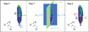 |
Fig. 1 Outflow selection slice perpendicular to the disk in run NOTURB, showing three of the eight steps to compute its opening angle. Displayed are the projection vector pi associated to cell i (Eq. (3), left panel), the four subselections based on this projection (middle panel) and the geometric center vector u, and two of the outermost positions vectors r2,± used to compute the opening angle (Eq. (4), right panel). The circle shows the sink position that we consider as the coordinates origin. |
2.2 Analysis: outflow properties
Section 3 is dedicated studying the outflows. We are looking at potentially fast (≳ 10 km s−1) outflows but we do not want to extract very biased properties by only selecting their higher-velocity component. Instead, we identify outflows on a cell-by-cell basis as follows. To be considered as part of an outflow, the radial speed within a cell must exceed the escape speed: vr > vesc with  , where r is the distance to the central star of mass M⋆. The velocity component perpendicular to the disk plane v⊥ must exceed a threshold of 0.8 km s−1. This value corresponds to the maximal velocity introduced in our turbulent initial conditions in runs SUPA and SUBA. We choose this value rather than that implied by Run SUPAS (≈ 3km s−1) in order to minimize the bias towards high-velocity gas when computing the outflow properties and because the outflow in Run SUPAS is weak and transient in a highly dynamical medium, making robust measurements difficult. Taking the component perpendicular to the disk strengthens this criterion, so that potential thermal-pressure-driven, radiative-pressure-driven, or interchange-instability-driven flows (see Paper I) occurring at the disk edge, parallel to the disk plane, are not counted as outflows. Thanks to this process, we can easily obtain the mean properties of the outflow. To go further and extract its geometry, we developed the method below.
Below we present our method to extract the outflow opening angle, trying not to make strong assumptions on the outflow geometry (e.g., conical, strictly perpendicular to the disk or to the axes, axisymmetric). Looking at bipolar outflows, we distinguish two components, each one located on one side of the disk plane, and compute their properties individually. We consider the primary sink as the origin, use ri to refer to the position vector of thecell of index i, and create the basis (e1, e2, e3) where e1 is colinear to the angular momentum vector J and e2, e3 are in the disk plane. For this computation, the angular momentum is taken as  where r and v are the position and velocity vectors, respectively.
- 1.
As detailed above, we first select all cells with vr > vesc and v⊥ > 0.8 km s−1.
- 2.
For each cell in the outflow selection, we compute the dot product between the position vector ri and J and create two subselections to distinguish the two cases: ri ⋅J > 0 (“above” the disk) and ri ⋅J < 0 (“below”) that we refer to as “A” and “B” outflows. Now we focus on one subselection between the two, i.e., one outflow.
- 3.
We define the position vector of geometric center (see Fig. 1)
 (1)
(1)where dVi is the volume of the cell of index i. We observe transient clumps of denser gas being ejected within the outflows; therefore taking the barycenter instead of the geometric center would lead to more variability and difficulty in interpreting the outcomes.
- 4.
We get the distance between the sink and the geometric center. We use this value as a sphere radius centered on the outflow geometric center and remove cells located outside the sphere: this acts as a connectivity criterion. In binary systems, we also exclude cells located within an orbital separation of the secondary star.
- 5.
Following the methodology of Cabrit & Bertout (1992), we get the distance of the most distant outflow cell Routflow and the volume-averaged velocity voutflow of the selection to compute the outflow momentum rate:
 (2)
(2)This corresponds to the required force to accelerate the flow from a null velocity to the characteristic velocity voutflow on a timescale of Routflow∕voutflow.
- 6.
We compute the projection pi (left panel of Fig. 1) of the cell position vector perpendicular to the position vector of the geometrical center u,
 (3)
(3) - 7.
We create four subselections pi,2 > 0, pi,2 < 0, pi,3 > 0, and pi,3 < 0 (middle panel of Fig. 1). The subscripts 2 and 3 denote the basis vectors e2 and e3, respectively.
- 8.
In the pi,2 > 0 subselection, we identify the cell with
 ; its position vector is labeled r2,+. This corresponds to the outermost cell in the positive e2 direction. We perform the same step for pi,2 < 0 (outermost cell in the negative e2 direction), pi,3 > 0 and pi,3 < 0, and obtain r2,−, r3,+, r3,− (right panel of Fig. 1).
 - 9.
We define the outflow opening angle θoutflow as the average of the four angles between u and r2,+, r2,−, r3,+ and r3,−, respectively, i.e.,
 (4)
(4)where the factor 2 arises because the four angles correspond to semi-opening angles.
Let us note that, by projecting the cell positions onto the disk plane (e2, e3), we implicitly assume that the outflow is perpendicular to the disk. As this is not generally valid, our resulting opening angle becomes less accurate as the misalignment between the outflow and j increases (see Sect. 3.6).
3 Results: outflow launching mechanism and observable properties
3.1 Analytical estimate of the origin
We aim to study the candidates for driving bipolar outflows: radiative acceleration, magnetic tower flow, and magneto-centrifugal acceleration. While modeling the latter requires strong assumptions on the magnetic field topology, we choose to compare the radiative and magnetic pressure-driven accelerations analytically.
The radiative and magnetic-pressure-gradient accelerations are respectively defined as arad = κF∕c = κL∕4πr2c where κ is the dust-and-gas mixture opacity, F is the radiative flux coming from the star, L is the stellar luminosity, r is the distance to the star, and apmag = 1∕ρ∇Pmag = 1∕ρ∇B2∕2. In the ideal MHD regime, B ∝ ρ2∕3 and ρ ∝ r−2 from our initial conditions, so B ∝ r−4∕3. It follows that the acceleration due to the magnetic pressure gradient can be approximated as
 (5)
(5)
Now comparing the radiative and magnetic accelerations absolute values and deducing the luminosity for the radiative acceleration to overcome the magnetic acceleration, one obtains
 (6)
(6)
taking r0 = 50 AU, B0 = 0.1 G, κ0 = 50 cm2 g−1 (the gray opacity to stellar radiation, considering an effective temperature of 4000 K), and ρ0 = 10−15g cm−3 as references after r0 has been fixed. From this equation, we can anticipate a change of regime from magnetic-dominated to radiation-dominated outflows as the protostellar luminosity increases, but only at small to intermediate scales. Indeed, Eq. (6) shows that the radiative acceleration decreases more rapidly with the distance than the magnetic acceleration, meaning that, at large distances, magnetic tower flow is the dominant mechanism. This analysis remains valid as long as the two components do not interact with each other. More specifically, the radiative force can push on the field lines and perturb the field topology (Vaidya et al. 2011), while the tower flow dense parts can shield the rest of the outflow from stellar radiation. More generally, the previous formulation is no longer valid for r > 1∕(κρoutflow) (optically thick outflow), except to show that the radiative acceleration is overwhelmed by magnetic-pressure gradient.
3.2 Fiducial case: run NOTURB
We start by analyzing the nonturbulent run NOTURB as our fiducial case, before comparing it with the study of C21 (their run MU5AD, with μ = 5).
3.2.1 Radiative acceleration versus Lorentz acceleration
Let us identify which of the two forces dominates when the star becomes massive (≳ 8 M⊙), in run NOTURB for simplicity. Figure 2 shows slices perpendicular to the disk plane of the ratios aLor∕agrav (left panel),which are the Lorentz and gravitational accelerations, respectively, aLor∕arad (middle panel) and arad∕agrav (right panel). The snapshots are taken when the central star is 10 M⊙ and L = 2 × 10⁴ L⊙ in run NOTURB and when M = 23.8 M⊙ and L =1.2 × 10⁵ L⊙ in run LRNOTURB. The radiative acceleration arad is the total (i.e., M1 and FLD) radiative acceleration. Run LRNOTURB allows us to reach a higher stellar mass and therefore a greater luminosity. One can clearly see that both the Lorentz force and the radiative force contribute to the gas acceleration in the outflow, as they exceed the gravitational force. Interestingly, in run NOTURB the radiative force contribution is very asymmetric with respectto the disk plane. This is due to the density distribution not being symmetric, with denser gas in the southern direction stopping stellar radiation propagation, while the northern direction is particularly optically thin at this time-step. We briefly discuss this asymmetry below. The extent of the radiatively dominated region is more constant with time in run LRNOTURB. Indeed, this reflects a fundamental problem when modeling radiative transfer: if the photon mean free path is not resolved, absorption is overestimated. Hence, there is more absorption in run LRNOTURB (a factor ≈ 2 at L = 2 × 10⁴ L⊙ in both runs). We measured the absorption by taking the photon density as a function of the distance to the sink to derive an absorption factor, assuming exponential decay and after correcting for geometrical dilution. This difference in absorption explains why, despite a larger stellar luminosity than in the run NOTURB snapshot, radiation does not propagate further away. As shown in the middle panel of Fig. 2, the Lorentz acceleration dominates the radiative acceleration everywhere except in the vicinity of the star (closer than ≈ 300 AU in run NOTURB). In the meantime, run LRNOTURB illustrates the stronger radiative force with a more extended zone where radiative force dominates over Lorentz force. The center panel and right panel show very similar features, revealing that the radiative force domination is limited by absorption in run LRNOTURB, while it is mainly limited by geometrical dilution (inherent to an optically thin channel) in run NOTURB. To conclude, the Lorentz force dominates over the radiative force up to a stellar mass of ~ 20 M⊙.
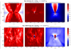 |
Fig. 2 Slices of 10 000 AU of three forces ratios when M = 10 M⊙ (L = 2 × 10⁴ L⊙) in run NOTURB (top) and when M = 23.8 M⊙ (L = 1.2 × 10⁵ L⊙) in run LRNOTURB. Left panels: Lorentz against gravitational acceleration. Middle panels: Lorentz acceleration against radiative acceleration. Right panels: radiative acceleration against gravitational acceleration. Lorentz acceleration dominates over the radiative acceleration everywhere but close to the protostar. |
3.2.2 Radiative acceleration: FLD versus M1
Above we consider the total numerical radiative acceleration from our two radiative transfer modules, but this can be decomposed as the sum of the stellar radiative acceleration and treated with the M1 module and the FLD radiative acceleration. The latter corresponds to momentum transfer from dust-reprocessed (infrared-like) radiation after stellar radiation (the main luminosity source in these simulations) has been absorbed. Figure 3 shows the ratio of FLD radiative acceleration to the gravitational acceleration (top panel) and to the M1 radiative acceleration (bottom panel). The FLD acceleration also contributes to the outflow, because it dominates over the gravitational force. Although its contribution is marginal compared to the direct stellar radiative force in the outflows here, it could play a more important role in the gas dynamics inthe regions shielded from stellar radiation. Indeed, the FLD acceleration is greater in the southern outflow where density is higher (see the density slices displayed in Figs. 4 and 5) because of the increased re-processed emission. In the same figure, we observe regions of higher outflow density (ρ > 10−18 g cm−3) than in purely radiative outflows (see e.g., Rosen et al. 2016; Mignon-Risse et al. 2020). As a consequence, stellar radiation is absorbed and cannot contribute to the gas acceleration at large (> 104 AU) distances when such a transient density region is present. The ejection of optically thick material is a common feature in our simulation, as we discuss below.
3.2.3 Magnetic tower flow
Now, let us focus on the magnetic launching mechanism. As shown in Fig. 2, the Lorentz force dominates the gas dynamics in the outflow. It can be decomposed as the sum of a magnetic-pressure gradient force and a magnetic tension force. While the former pushes the gas along the direction of stronger magnetic fields variations, giving rise to a magnetic tower flow, the latter impedes the bending of the field lines. The left panel of Fig. 6 shows the ratio of the magnetic-pressure-gradient force to the gravitational force in the direction perpendicular to the disk, computed from simulations outputs. We only take the toroidal component of the magnetic field (in the frame of the sink), as it is the only one contributing to the gas dynamics in the poloidal direction (Spruit 1996). This acceleration appears to dominate over gravity in the whole of the outflow by about one order of magnitude. Therefore, the outflow in our simulation contains a magnetic tower flow (Lynden-Bell 1996, 2003). As shown in the right panel of Fig. 6, the toroidal component (blue) indeed dominates the outer zones of the outflow, while the poloidal component dominates close to the outflow axis. In that respect, we obtain a similar outflow magnetic structure as many works in the literature (see e.g., Seifried et al. 2012). From the left panel of Fig. 6 it can be seen that the tower-flow-launching region (i.e., close to the disk plane y ~ 0) is not restricted to the inner disk region because the disk radius in run NOTURB is ≈ 100 AU (see Paper I), while the region where this acceleration dominates over gravity (the red region) extends over more than 1000 AU perpendicular to the outflow. This is consistent with the toroidal component of the magnetic field dominating beyond the disk outer radius (up to ≈ 500 AU, see Fig. 13 of Paper I). More precisely, the tower flow develops on disk scales and widens later on. As in Kato et al. (2004), we find that the outflow itself is dominated by magnetic pressure (β = Pth∕Pmag < 1, where Pth and Pmag are the thermal and magnetic pressures, respectively, while the outflow edge corresponds to β ≈ 1), as displayed in Fig. 7. In addition to the possible thermal pressure gradient from the outer medium, collimation is enforced by the magnetic tension force when the field lines are sufficiently wound up. While we emphasize the poloidal (i.e., pressure-driven) component of the Lorentz acceleration in the left panel of Fig. 6, there is a collimating component as well, as can be seen from the direction of the Lorentz acceleration vectors in Fig. 7. The tower grows vertically (i.e., the frontier between the outflow and the outer medium) as the field lines anchored on the disk rotate, and the tower vertical growth is predicted to occur at the disk rotation velocity (Lynden-Bell 1996). Indeed, looking at the evolution of the tower frontier position over 32 kyr, we find a mean growth velocity of ≈ 6 km s−1. In the meantime, we reported a gas azimuthal velocity in the disk of ≈5 km s−1 at the outer radius. This is consistent with the findings of Lynden-Bell (1996).
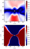 |
Fig. 3 Slice of 1000 AU showing the ratio of the FLD radiative acceleration to the gravitational acceleration (top) and to the M1 radiative acceleration (bottom), perpendicular to the disk plane in run NOTURB, when M = 12.7 M⊙. Below M = 10 M⊙, the FLD radiative acceleration rarely dominates the gravitational acceleration. The M1 acceleration dominates in the outflow region over the FLD acceleration and the disk region is dominated by the FLD acceleration. |
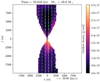 |
Fig. 4 Gas density slice of 20000 AU in the outflow selection perpendicular to the disk plane: run NOTURB, M = 10 M⊙. The gas outflow density corresponds to particle densities between ~105 cm−3 and ~ 107 cm−3. |
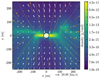 |
Fig. 5 Gas density slice of 500 AU perpendicular to the disk plane: run NOTURB, M = 10 M⊙. Velocity vectors and magnetic lines are overplotted. The gas density corresponds to particle densities between ~ 106 and ~ 1013 cm−3. |
3.2.4 Magneto-centrifugal outflow
As the poloidal magnetic field component dominates close to the outflow axis and in the disk midplane (right panel of Fig. 6), we investigate whether the magneto-centrifugal process originally described by Blandford & Payne (1982) is at work. In this process, gas is centrifugally accelerated along field lines anchored in the disk and corotating with it. Distinguishing centrifugal acceleration from a magnetic tower acceleration is a complicated task in such adaptive mesh refinement calculations,as underlined by Seifried et al. (2012). Indeed, the system is far from the ideal MHD, axisymmetric stationary case and the criterion from Blandford & Payne (1982) only applies to the disk surface. These latter authors derived strict conditions in terms of theinclination of magnetic field lines to launch the flow centrifugally, but neglect disk thermal pressure which is non-negligible in our calculation. Moreover, analytical results rely on several invariants along the field lines (see e.g., Ogilvie 2016), but it is difficult to trace the field line on which a gas particle has been centrifugally accelerated back to the line foot point in the disk. For that purpose, Seifried et al. (2012) derived a criterion to estimate whether centrifugal acceleration is taking place based on grid-evaluated quantities. These authors assume that Bϕ = 0, so that the field lines corotate with the gas. As Bϕ is never strictly equal to zero in our calculation, we apply this criterion only where Bp > Bϕ. The aim of Seifried et al. (2012) is to determine, for a given point, the isocontour along which the effective gravity (accounting for the centrifugal force) is constant: it draws a line along which gas can freely move, regarding these forces. They then compare, in the (r, z)−plane (in cylindrical coordinates), the gas trajectory along this line to the field lines inclination by computing the derivative ∂z(r)∕∂r to Bz ∕Br, where z(r) is given by theisocontour equation (Eq. 16 of Seifried et al. 2012). Eventually, at any given point, centrifugal acceleration occurs if ∂z(r)∕∂r is larger than the field line inclination, i.e.,
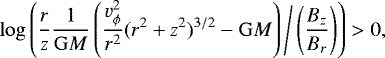 (7)
(7)
where the numerator corresponds to ∂z(r)∕∂r. We visualize this criterion in Fig. 8: centrifugal acceleration occurs in red regions. Hence, the zone close to the outflow axis, where we previously found Bp to dominate, is consistent with centrifugal acceleration.
In the cold disk limit, gas is accelerated centrifugally from the disk surface to the Alfvén point, where the poloidal velocity equals the poloidal Alfvén speed. We check this by visualizing these velocities as a function of the (mainly vertical) distance to the sink. As shown in Paper I, Bp dominates for disk radii ≲50 AU, and therefore the centrifugal mechanism may be at work below 50 AU. Therefore, we select cells at a cylindrical radius smaller than 100 AU, so that theirexpected launching radius is a few tens of AU, which is consistent with the zone where the magnetic field is mainly poloidal within the disk. Figure 9 shows these velocities in the northern (A) and southern (B) outflows of run NOTURB when M = 10 M⊙. The poloidal velocity is found to increase when the distance to the sink is larger than 60− 80 AU. Gas acceleration appears to take place up to the Alfvén point, in agreement with the theory (e.g., Spruit 1996). As shown in the right panel of Fig. 6, even beyond the Alfvén surface (≳ 1000−2000 AU), the poloidal component dominates close to the outflow axis. This feature is reminiscent of the findings of many studies including a magnetic tower flow (e.g. Kato et al. 2004; Banerjee & Pudritz 2007; Seifried et al. 2012; Kölligan & Kuiper 2018). A plausible explanation for the generation of the poloidal component close to the axis (beyond the Alfvén surface) is the vertical inflation of the magnetic tower which develops the magnetic field poloidal component as it grows (Kato et al. 2004). Consistently, we find a nearly perfect alignment between the velocity vector and the magnetic field vector close to the outflow axis, while it is nearly perpendicular further away from the axis. This suggests that gas located near the axis is accelerated magneto-centrifugally.
The magneto-centrifugal mechanism is the best candidate for the fast outflows around young-stellar objects. We therefore compare the highest velocities we obtain with theoretical predictions. The terminal velocity v∞ is predicted tobe (e.g., Pudritz et al. 2007)
 (8)
(8)
where rc,A is the (cylindrical) Alfvén radius and rc,0 is the launching radius, so that rc,A∕rc,0 is the lever arm and has a typical value of 2−3 (Pudritz & Ray 2019), and vesc,0 is the escape velocity at the launching distance. Magneto-centrifugal outflows have an onion-like velocity distribution, with the highest speed close to the axis corresponding to the gas initially close to the central object. In our simulation, gas is launched at a vertical distance of 60− 80 AU from the sink (see also Fig. 5). Hence, we infer a corresponding escape velocity of ≈ 11 km s−1 for M = 10 M⊙. This leads to v∞ ≃ 22−33 km s−1, which is of the same order as the fastest velocities we obtain at this time-step, namely v ~ 32 km s−1 on one side of the disk and v ~ 20 km s−1 on the other side (Fig. 9). Hence, the magneto-centrifugal mechanism may be responsible for the highest velocities of outflow, close to the axis, while the magnetic tower flow drives the wider angle and slower component of the outflow. Moreover, the wide-angle gas is unlikely related to magneto-centrifugal acceleration because it can be located more than 2000 AU away from the axis (see Fig. 4), which is inconsistent with a launch from a 100 AU disk with a lever arm of 2−3 as predicted by the theory.
Let us note that the highest velocity in each lobe shows fluctuations between these two values. These small velocity differences suggest thatthis mechanism may be either transient in our simulation (the radiative acceleration being able to accelerate the gas to v ~ 20 km s−1) or not symmetric with respect to the disk plane (as can be seen in Fig. 4). This north–south asymmetry in the ejection may arise from the asymmetry in the streamers. These channels feeding the disk are not located in the disk plane (more details in Paper I), hence part of the outflow asymmetry may be a product of this asymmetry.
Let us also recall that the magneto-centrifugal mechanism taps into the gravitational energy, as can be seen from the relation above between the outflow terminal velocity and its initial escape velocity. Hence, a launch from the disk (~ 20 AU for the disk inner edge) instead of ~100 AU above it would result in a more than twice larger initial escape velocity (and therefore a twice larger terminal velocity). Overall, there are several clues indicating the presence of a magneto-centrifugal jet in our simulation.
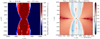 |
Fig. 6 Left panel: ratio of the magnetic-pressure-gradient acceleration and the gravitational acceleration in the vertical direction. Right panel: ratio of the poloidal and toroidal components of the magnetic field and velocity vectors overplotted. Slices of 20 000 AU perpendicular to the disk plane are shown, when M = 10 M⊙; run NOTURB. |
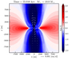 |
Fig. 7 Plasma β and Lorentz acceleration vectors overplotted. Slice of 20 000 AU perpendicular to the disk plane, when M = 10 M⊙, run NOTURB. |
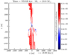 |
Fig. 8 Criterion for centrifugal acceleration (Eq. (7)) from Seifried et al. (2012) applied to a slice of 4000 AU perpendicular to the disk plane. Run NOTURB, M = 10 M⊙. Red regions are consistent with centrifugal acceleration. |
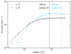 |
Fig. 9 Poloidal velocity as a function of the distance to the sink (mainly in the vertical direction), in a cylindrical selection of cells with rcyl < 100 AU. Negative radial velocities have been masked out. Velocities are obtained as averages over a distance bin. A and B label the northern and southern outflow, respectively, and the vertical lines indicate the positions where the poloidal velocity equals the Alfvén poloidal velocity (averaged over the same distance bin). Run NOTURB, M = 10 M⊙. |
3.3 Influence of a turbulent medium: runs SUPA, SUPAS, and SUBA
We now focus on the outflows in the three other runs. Figure 10 shows density slices in the outflow selection (left panel), the ratio between the Lorentz and the radiative accelerations (middle panel), and the ratio between the radiative and the gravitational accelerations (right panel). We recall that the Lorentz acceleration encapsulates the magnetic pressure gradient acceleration. Outflows form at t ~ 30 kyr in the subAlfvénic runs, NOTURB and SUBA. Meanwhile, their launch occurs at t = 56 kyr in run SUPA and ~66 kyr in run SUPAS (see Table 2).
The inclusion of a noncoherent initial velocity distribution in our turbulent runs should perturb the magnetic field coherence, impeding the launch of the outflow. As shown in Fig. 13 of Paper I, ~ 22 kyr after sink formation a strong toroidal magnetic field has built up, but no outflow has been launched yet in runs SUPA and SUPAS. Indeed, the density structure formed by the combined effect of infall and turbulent motions is a filament-like structure of a few thousand AU almost perpendicular to the disk plane, which carries an additional ram pressure to be overcome by the outflow regardless of its origin.
Magnetic and radiative forces are of different nature. On the one hand, magnetic outflow launching is a long-term process and can be prevented, for example, by the orbital motions in a binary system (Peters et al. 2011). On the other hand, the launching (close to the star) of radiative outflows is isotropic and depends mostly on the density distribution via the optical depth. Its launch and propagation depend on the environment, and so one can expect transient and smaller radiative outflows in a turbulent medium, unless radiation can find its way out and accelerate gas instantaneously. Without magnetic fields, Rosen et al. (2019) found that infalling filaments of gas are self-shielded against radiation and form a network of dense filaments and optically thin channels centered on the massive star.
In the present study, with magnetic fields and super-Alfvénic turbulence (run SUPAS), gravity is diluted and material gently falls via thermally supported (β > 1) streamers on a moderately magnetized complex structure of ~1000 AU squared (see Fig. 2 of Paper I). At that time, a secondary star–disk system has formed. As a consequence, we observe two failed attempts at launching outflow as dense gas passes through it. These occur when the secondary sink is closer to the apastron. Eventually, the monopolar outflow launches, and survives for ~ 3 kyr before it becomes difficult to characterize it as an outflow because it has been perturbed by the environment motions and no gas is newlyejected from the basis. A similar process occurs in run SUPA. While the ram pressure is lower than in run SUPAS and consequently an outflow successfully develops, the formation of a secondary sink at about the same time has progressively displaced the center of mass of the system. The primary sink disk moves on a ~ 350−600 AU orbit and the outflow is consequently broadened from the basis. Nonetheless, the outflow is sustained until the end of the run, as opposed to run SUPAS. As mentioned above, the orbit is eccentric. When the primary sink approaches the apastron, it stays longer in the same area and has more time to accelerate the gas radiatively. Finally, despite the turbulent support, the subAlfvénic run SUBA has no difficulty launching the outflows at about the same time as in the fiducial run, because the initial magnetic field is stronger. The toroidal magnetic field reaches similar values as in the less-magnetized, nonturbulent run NOTURB (> 0.1 G). The magnetic tower develops at about the same speed as in run NOTURB. The presence of a turbulent velocity field contributes to the north–south asymmetry. The bipolar outflows, which are not strictly identical in run NOTURB, are even more distinguishable in terms of extent or orientation here. Hence, turbulence provides an additional mechanism to break the symmetry between bipolar outflows and can even suppress them.
Figure 10 shows that once the outflows are launched in runs SUPA and SUPAS, the local relative contribution from radiative acceleration to the total acceleration is larger than in the fiducial case. First, by delaying the launching, the central star has time to reach slightly higher masses (and therefore luminosities). Second, the magnetic field is less organized than in the nonturbulent case, and thus the component of the Lorentz force contributing to the outflow is smaller.
Let us compare the two accelerations in the outflow as a function of time. Figure 11 shows the ratio between the radiative acceleration and the Lorentz acceleration, both integrated over the outflow volume, as a function of the primary sink luminosity. In our simulations, the sink luminosity is an increasing, monotonic function of time. This figure shows that the Lorentz acceleration is significantly greater (two orders of magnitude) than the radiative acceleration at the time when the outflow forms. In run SUPA, the ratio approaches one. This is due to the outflow having formed later than in the other runs, so the outflow is smaller and radiative acceleration is efficient. We observe that, even for a luminosity larger than 104 L⊙, the Lorentz acceleration dominates in the outflow.
As in run NOTURB, we find that the poloidal component of the magnetic field dominates the toroidal component close to the outflow axis and in the disk plane (see Paper I) in runs SUPA and SUBA. This suggests that the magneto-centrifugal mechanism could be at play, in addition to the Lorentz acceleration.
To conclude, turbulence delays the outflows but does not change their nature: we still obtain magnetic outflows, although the local relative contribution from radiative acceleration is larger than without turbulence.
 |
Fig. 10 Slices perpendicular to the disk plane. Left column: density slice in the outflow selection. Middle column: ratio of the Lorentz acceleration to the radiative acceleration. Right column: ratio of the radiative acceleration to the gravitational force. From top to bottom: Run SUPA (super-Alfvénic, subsonic turbulence, 10 000 AU, t = 67.0 kyr, M = 8.2 M⊙, L = 1.4 × 10⁴ L⊙), run SUPAS (super-Alfvénic, supersonic turbulence, 4000 AU, t = 72.6 kyr, M = 5.6 M⊙, L = 8 × 10³ L⊙) and run SUBA (sub-Alfvénic, subsonic turbulence, 10 000 AU, t = 61.1 kyr, M = 9.6 M⊙, L = 1.7 × 10⁴ L⊙). The gas densities in the left column correspond to particle densities between ~ 104 and ~ 106 cm−3. |
Simulation outcomes regarding the outflow launching.
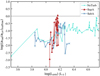 |
Fig. 11 Ratio between the radiative and Lorentz accelerations (both integrated over the outflow volume) as a function of the sink luminosity. |
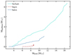 |
Fig. 12 Outflow mass as a function of the sink mass. |
3.4 A channel for radiation?
The magnetic outflows develop at a smaller stellar mass (M ≈ 4−7 M⊙, see Table 2) than what is found in RHD simulations regarding radiative outflows (M > 10 M⊙, see e.g. Kuiper et al. 2012; Mignon-Risse et al. 2020). Hence, they could act as a channel of radiation to propagate, as put forward by Krumholz et al. (2005) for protostellar outflows. Banerjee & Pudritz (2007) proposed the same mechanism for tower flows, but their calculation did not include radiative transfer. Despite the regular presence of optically thick gas in the outflow, most of the outflow volume is optically thin. To assess the effect of the radiative force, we compare theoutflow extent between the NOTURB run and one including the FLD method rather than the hybrid method (that we call the NOTURBFLD run; see the Appendix A.1). When the central star is ~ 5 M⊙, the outflow extends over more than ~4500 AU in the NOTURB run while it extends over 3000 AU in run NOTURBFLD (see Fig. A.1). Moreover, the outflow appears more symmetric (axisymmetric and north–south) in the NOTURB run than in the NOTURBFLD run, indicating that the radiative force stabilizes the outflow structure. To sum up, the outflow appears as a channel for radiation to escape. Radiative acceleration participates in the gas acceleration more than in the FLD case, as we find that the highest gas velocity is 25% smaller in run NOTURBFLD than in NOTURB (see Appendix A.1).
3.5 Outflow properties
3.5.1 Outflow mass
Figure 12 shows the outflow mass as a function of the sink mass. It generally increases with time and has values 1− 8 M⊙ in subAlfvénic runs and subsolar masses in run SUPA during the epoch covered. While it appears to be variable in run SUPA, it only increases in subAlfvénic runs, and more rapidly in the nonturbulent run NOTURB. We note that step 4 of our outflow definition (removing cells far from the outflow geometric center and close to the secondary sink) is required to obtain relevant measurements of outflow mass in run SUPA. Without this criterion, the outflow mass is larger by one order of magnitude because of the fact that we only loosely account for the dense gas gravitationally bound to the secondary sink. Considering their mass and dynamical time (i.e., timescale of existence), we obtain a mean ejection rate of ~ 2 × 10⁻⁴ M⊙ yr−1 in run NOTURB, ~ 5 × 10⁻⁵ M⊙ yr−1 in run SUBA, and ~ 10−5 M⊙ yr−1 in run SUPA.
It can be noted that around 11 M⊙ and 10 M⊙ there is a small change of slope in the outflow mass evolution in runs NOTURB and SUBA, respectively. Interestingly, radiative outflows are reported to occur at about this mass in radiation-hydrodynamical simulations (Kuiper et al. 2012; Mignon-Risse et al. 2020 with the same pre-main sequence track as here, i.e., taken from Kuiper & Yorke 2013). Hence, the change of slope, and more specifically the increase in the outflow-mass-to-sink-mass ratio may be linked to the increasing radiative force. An argument in that regard comes from the comparison with C21. These authors measure an outflow mass of ~ 2 M⊙ when the sink is ~8 M⊙, which is similar to what is obtained here. As the main difference between our runs comes from the radiative transfer method used, and the Flux-Limited Diffusion underestimates the direct stellar force compared to the hybrid method, this change of slope appearing at the stellar mass of ~20 M⊙ instead of ~10 M⊙ is consistent with a radiative force origin.
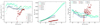 |
Fig. 13 Outflow properties as a function of the primary sink age: momentum rate (left), maximal outflow radius (middle), opening angle (right), and angle between the outflow and the large-scale magnetic field (bottom-right), in runs NOTURB, SUPA, SUBA. Forces and opening angles of outflows composed of less than 50 cells are not displayed. Outflows come in pairs in these runs, so they are individually labeled as A and B. Values are averaged over 0.5 kyr (smaller than the orbital timescale in run SUPA). |
3.5.2 Momentum rate
Left panel of Fig. 13 displays the outflow momentum transfer rate (also called outflow force) computed from Eq. (2), each point corresponding to an outflow (either northern, labeled “A” or southern, “B”) at a given time-step. For runs NOTURB and SUBA, we have Foutflow of the order of 10−4 M⊙ km s−1 yr−1 and a dispersion of less than one order of magnitude. We observe more dispersion at the beginning of run SUPA, and then the evolution is similar with an overall increasing force with time. By the end of run SUPA, the outflow force reaches similar values as in runs NOTURB and SUBA with ~10−4 M⊙ km s−1 yr−1. These are consistent with the aforementioned numerical work of Seifried et al. (2012).
3.5.3 Opening angles
Close to the star, the outflow shape resembles a conical shape before collimation occurs (≲ 2000 AU) and extends the outflow in an elliptic shape. In Sect. 2.2 we presented our method to compute the outflow opening angle (see also Fig. 1). We adopted a method adapted to the elliptic shape of the outflows we observe, which is similar to Offner et al. (2011).
The right panel of Fig. 13 shows θoutflow as a function of the sink age. We mentioned above that the outflow launched was quite similar between runs NOTURB and SUBA. Consequently, the values and evolution of the opening angle are, to first order, similar. During a first phase (a few kyr), the outflow broadens and so θoutflow increases; then (after a sink age ofroughly 9 kyr in run NOTURB, or 11 and 16 kyr in run SUBA) the base of the outflow becomes nearly stationary but the outflow propagates, and hence the opening angle decreases. During this second phase, the angle has values of 20–40deg which are north–south asymmetric. Finally, it tends toward 20− 25deg. The outflow re-collimates, which is partly due to the toroidal component of the magnetic fields (Fig. 7) and possibly to the pressure from the outer medium, in addition to the aforementioned geometrical effect. In run SUPA, the measurement of the opening angle is greatly affected by the orbital motions of the sink because the orbital separation (as large as 600 AU) is not negligible with respect to the outflow extent (~2000 AU, middle panel of Fig. 13), and the orbital velocity is similar to the tower growth speed, by definition (Sect. 3). As both velocities and spatial extents are of the same order, the outflow geometry becomes complex. Hence, the opening angle in run SUPA is not comparable to a single observation. If anything, it shows that the stellar motions in a turbulent medium, or a multiple stellar system, will strongly affect this type of geometrical measurement. Overall, we obtain opening angles varying between 30 deg and 70 deg and between the north and south outflow. The orbital motion seems to have played a dominant role in the outflow broadening. We focus on the outflow orientation in the following section.
3.6 Alignment with magnetic fields, core-scale angular momentum, and disk
Low- and high-mass pre-stellar cores are threaded by magnetic fields, but their exact role is not yet clear. As disk-mediated accretion is observed in the low-mass regime (e.g., Pety et al. 2006), and now in the high-mass regime as well (see e.g. Cesaroni et al. 2017), and disks are required to launch MHD outflows (supported by e.g., Hirota et al. 2017), studying the alignment between outfows and magnetic fields should provide insights into their exact role during (massive) star formation. Furthermore, magnetic outflows are expected to be launched perpendicular to the disk. In the following, we study the misalignment between outflows and magnetic fields, angular momentum (on core scale), and the disk. Figure 14 shows the angle formed by the outflow geometric center vector with respect to the x-axis (corresponding to the initial magnetic field orientation, left panel), with respect to the core-scale angular momentum vector (middle panel), and with respect to the disk normal vector (right panel), as a function of time.
In run NOTURB, we find a nearly perfect alignment between the outflows and the magnetic fields, the core-scale angular momentum, and the disk normal. Several factors have broken the north–south symmetry as well as the axisymmetry (which could increase the outflow-disk misalignment), but still the misalignment is smaller than 10 deg in each case and the bipolar outflows show similar misalignment angles.
Let us now study the misalignments in the turbulent runs. In run SUPA, the bipolar outflows are not symmetric and there is no clear trend toward an alignment with the large-scale magnetic fields. Most of the time, the outflows align within less than 40 deg with the disk normal and with the core-scale angular momentum.
In run SUBA, the angles between the outflows and both magnetic fields, and core-scale angular momentum decrease with time (but never reach a perfect alignment), suggesting a preference for outflow-angular momentum and outflow-magnetic field alignments on large scales. This is naively expected because magnetic outflows are related to organized field lines twisted by rotation. Here is another possible interpretation, based on the presence of streamers (dense filaments) perpendicular to the magnetic fields (see Fig. 2 of Paper I), randomly oriented with respect to the disk. Streamers may either enforce forbidden directions for the outflows by opposing a strong ram pressure, and these forbidden directions are 90 deg oriented with respect to the magnetic fields, or bring angular momentum and contribute to twisting of the field lines. By preventing outflow launching along these directions, the outflow center of mass is shifted toward a location closer to the magnetic fields axis. This trend is not visible in run SUPA, where the angles do not show any clear evolution other than periodic variations on orbital timescales.
Finally, a few words on the short-lived (≈3 kyr) monopolar outflow in run SUPAS. It develops almost perpendicular to the disk (with a disk–magnetic-field misalignment of ~ 90deg; see Paper I). This shows that, indeed, a disk oriented perpendicular to the core-scale magnetic fields has trouble launching outflows; but it remains possible (Joos et al. 2013). It can also occur on smaller scales than those covered in this study, especially in the case of magneto-centrifugal jets where the highest velocity component comes from the disk inner radius.
In summary, in the four runs, the outflow orientation appears to be mainly set by the disk orientation, which depends on the initial angular momentum. Nonetheless, it never corresponds to a strict perpendicular angle with the disk, and is larger in the super-Alfvénic run than in the subAlfvénic run. As the outflow grows, it tends to align with the core-scale magnetic fields and angular momentum when turbulence is subAlfvénic. Overall, the alignment with the disk normal and with the core-scale angular momentum (which is linked to the disk normal, as shown in Paper I) are better than with magnetic fields.
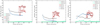 |
Fig. 14 Angle between the outflow and the large-scale magnetic field (left), the core-scale angular momentum (middle), and the disk (right), respectively, in runs NOTURB, SUPA, SUBA. Values obtained for outflows composed of less than 50 cells are notdisplayed. Outflows come in pairs in these runs, so they are individually labeled as A and B. |
4 Comparison of the outflow properties with observational constraints
In the following, we compare the outflows properties to the findings of several observational studies based on large samples of low- and high-mass protostars. When comparing to low-mass objects, we implicitly assume a continuity in the outflow-launching mechanism from low- to high-mass protostars, as pointed out by many studies (i.e., Cabrit & Bertout 1992; Bally 2016).
4.1 Outflow velocity, mass, dynamical time, and ejection rate
As mentioned in the previous section, the outflows in our simulations are dominated by MHD processes while radiation can participate in the acceleration. Before comparing the outcomes of our simulations with observational values, let us specify that some of these observable quantities are often plotted against stellar luminosity (see e.g., Lada 1985). Luminosity is not solely used as a tracer of evolutionary stage. As high-mass protostars are expected to have higher accretion rates than their low-mass counterparts (Motte et al. 2018), the luminosity has often been used as a proxy for the accretion rate (Wu et al. 2004). This is of utmost interest here because MHD disk outflows are powered by the gravitational energy from accretion, with a predicted ratio of mass outflow rate to mass accretion rate ~ 0.1 (see Pudritz & Ray 2019 and references therein). Matsushita et al. (2017) obtain a ratio of ≳ 0.2, which can approach unity when the core initial magnetic energy is comparable to the gravitational energy. Finally, we refer to a mean accretion or ejection rate by run rather than an instantaneous rate, as it can vary by more than one order of magnitude from one time-step to another (see Paper I).
First, as shown in the left panel of Fig. 8, the maximal outflow velocity vmax in run NOTURB is ≃ 20 km s−1 for one outflow lobe and ≃ 32 km s−1 for the other, at the time when the central star is 10 M⊙. This velocity is expected to gently increase with the squared root of the sink mass for magnetic outflows; after a sudden increase phase (until Msink ~6 M⊙), we find 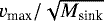 to remain constant within ~20%. We compare the previous values with those obtained by Nony et al. (2020) on the most massive core (~ 102 M⊙) of their 1− 100 M⊙ sample (in the W43-MM1 protocluster). On this sample, they obtained a median velocity of 47 km s−1. The most massive core exhibits a monopolar outflow with a maximal velocity of 34 ± 2km s−1 and 10 000 ± 1000 AU length, which agrees well with one of the two outflow lobes in run NOTURB (when the central star is 10 M⊙). Interestingly, while we attribute the monopolar nature of the outflow in run SUPAS to the ram pressure of the turbulent gas, this occurrence in W43-MM1 could be due to an inflow of material according to Nony et al. (2020).
Let us first present the observational results regarding outflow masses before comparing with our study. Wu et al. (2004) built a statistical study of 391 high-velocity outflows covering several evolutionary stages. For L > 103 L⊙ objects, these latter obtain outflow masses of a few solar masses up to 102 M⊙ with averaged dynamical times of 100 kyr. This is consistent with the study of Beuther et al. (2002) which focused on the CO J = 2−1 emission towards 26 massive star-forming regions. These authors obtain outflow masses of typically  (where Mc is the core mass) and dynamical timescales of the order of the core free-fall time. In the sample of 11 massive star-forming regions of Wu et al. (2005), the outflow mass is also found to be between a few solar masses, while the maximal mass is 60 M⊙ and averaged dynamical timescales are of 20 kyr. Similarly, Zhang et al. (2005) extract a mean outflow mass of 20.6 M⊙ and a median of 15.6 M⊙ from a sample of 69 sources with luminosities of 102−5 L⊙.
The upper-mass limits of 60−100 M⊙ are significantly larger than what we obtain, as well as those obtained by Zhang et al. (2005) of 15.6−20.6 M⊙, although the latter values might be reached at later times in our study (this would occur at M ~ 21 M⊙ in run NOTURB, extrapolating from the results presented in Fig. 12). The outflow mass presented in Beuther et al. (2002) for a core mass similar to ours (Mc = 100 M⊙, corresponding to L > 103 L⊙ from their Fig. 4) is ~4 M⊙ (see the relation above), which is consistent with our results for subAlfvénic runs (Fig. 12), and possibly for run SUPA at later times. All these studies agree on typical accretion rates of a few times 10−4 M⊙ yr−1, similar to those presented in Paper I. Hence, regarding the outflow mass, our outflows are consistent with observational constraints.
On the one hand, the outflow ejection rate is consistent with observations of high-mass cores and luminous (> 102 L⊙) protostellar objects. On the other hand, the outflow mass agrees when the core mass is 100 M⊙ (Beuther et al. 2002), and is smaller than for more massive cores. This discrepancy can be explained by our initial conditions corresponding to the low-mass limit of massive cores.
4.2 Outflow momentum rate
Let us compare the results presented in Sect. 3.5.2 with the current observational constraints (observed in CO) for L >103 L⊙ objects. Indeed, the pioneer study of Lada (1985) revealed a general trend between the outflow force and the stellar luminosity of Foutflow~102L∕c from 1 L⊙ to 105 L⊙, suggesting a common outflow mechanism for low- and high-mass protostars, which is likely a magnetic mechanism. Hence, let us determine whether our outflow forces are consistent with this trend, with up-to-date outflow samples. In the statistical analysis of Wu et al. (2004) towards high-velocity outflows, 102 M⊙ is the lowest core mass of the sample and gives FCO = 10−3 M⊙ km s−1 yr−1. Towards 11 massive star-forming regions, Wu et al. (2005) found values of between ~10−3 M⊙ km s−1 yr−1 and 2 × 10⁻¹ M⊙ km s−1 yr−1 (for L > 103 L⊙ protostars). Including the measurements from Beuther et al. (2002); Zhang et al. (2005) obtain outflow forces of 10−4−10−2 M⊙ km s−1 yr−1. Hence, the outflow momentum rate we obtain is consistent with the lower values mentioned above, that is 10−4 M⊙ km s−1 yr−1. However, we note that the uncertainty is almost two orders of magnitude on the values of Wu et al. (2005). Further observational campaigns are required to put stronger constraints on the outflow force.
4.3 Opening angles
Collimated outflows are observed around O- and B-type protostars (Arce et al. 2007), but several studies point toward less collimated outflows in the high-mass regime than in the low-mass regime (see e.g., Beuther et al. 2002; Wu et al. 2004). Opening angles of between 17deg and 25deg (i.e., a good collimation) have been reported in the massive protostellar sources IRAS 20126+4104 (Moscadelli et al. 2005) and IRAS 16547-4247 (Rodriguez et al. 2005), but likely originate from a magneto-centrifugal jet given the velocities involved (34–112 km s−1 for IRAS 20126+4104).
The outflow morphology below ~2000 AU in runs NOTURB and SUBA roughly fits a conical shape. The outflow growth, while keeping this shape, lasts a few thousands years. This epoch corresponds to the highest values of θoutflow measured, with θoutflow≈30−60deg until then. For comparison, Pety et al. (2006) (in the low-mass regime) fit a conical shape to an outflow of ~ 450 AU for a low-mass protostar, with an opening angle of 60deg. If the outflow mechanism is indeed the same for low- and high-mass stars, and if this is a magnetic tower flow, then the outflow detected by Pety et al. (2006) should re-collimate at larger radii and later times if accretion continues.
Wu et al. (2004) and Beuther et al. (2002) find average opening angles of ~ 53deg over the same samples of >103 L⊙ sources (corresponding to 5−15 M⊙ protostars in Wu et al. 2004) mentioned above; however these are higher limits due to angular resolution and projection effects (Beuther et al. 2002). These are typically larger than what we obtain in runs NOTURB and SUBA. Therefore, this discrepancy may indicate a different outflow-launching process, a smaller pressure confinement by the outer medium, or a need for higher numerical resolution at the outflow–environment interface in our simulation if these values were to be confirmed with higher angular resolution studies.
4.4 Alignment with magnetic fields, core-scale angular momentum, and disk
Let us now compare the values obtained in Sect. 3.6 to observational studies, in both the low- and high-mass regimes, because, as we see below, so far there is no suggestion of a different orientation mechanism depending on the stellar mass. In the low-mass regime, Hull et al. (2013) observe that the angle distribution between outflows and magnetic fields on scales of ~ 1000 AU is consistent with random distribution or preferentially perpendicular, on a sample of 16 low-mass protostars. On the core-scale, Hull et al. (2014) reached a similar conclusion. With a sample of four low-mass isolated protostars, Chapman et al. (2013) came to the opposite conclusion, with a positive correlation between the outflow axis and the magnetic field direction. Interestingly, Galametz et al. (2018) show that the best alignment between the magnetic fields and the outflow axis is observed for sources with no large (> 100 AU) disk or multiplicity. Finally, in the high-mass regime, Arce-Tord et al. (2020) reach the same conclusions as Hull et al. (2014): their distribution is best fitted by either a 50−70deg preferential orientation or a random orientation between the outflow and the magnetic fields.
To begin with, our results seem to favor a random inclination on small scales, as observed by Hull et al. (2013), because the outflow orientation is initially set by the disk orientation, which depends on the initial momentum carried by turbulence. Second, the sample of Chapman et al. (2013) is most likely comparable to our nonturbulent run NOTURB, because these latter authors only investigate protostars that are isolated (e.g., B335, Olofsson & Olofsson 2009), while we show in Paper I that turbulence favors the formation of multiple stellar systems. Therefore, the positive correlation between the outflow axis and the magnetic fields in Chapman et al. (2013) agrees with our results. Moreover, the present study is consistent with the observations of Galametz et al. (2018). In fact, we only observe large rotating structures and multiple systems for super-Alfvénic runs, for which the outflow–magnetic field misalignment is indeed larger than in the subAlfvénic runs. Overall, our work would suggest that the preferential perpendicular orientation (> 45deg) or random orientation would be obtained for systems with the Alfvénic Mach number  , as a consequence of the outflow being perpendicular to the disk, whose orientation is set by the initial angular momentum. On the contrary, it would suggest that a better alignment is obtained for
  , because the field line geometry or the streamers (perpendicular to B) re-orient the outflows towards the core-scale magnetic field axis.
Finally, let us take a look at the magnetic field strength within the outflow. As the outflow grows, its mean magnetic field strength decreases. We measure a mean field strength of 15 mG in run NOTURB at the time when the outflow reaches ~ 2000 AU, and 5 mG when it reaches ~ 5000 AU. Using the Chandrasekhar-Fermi method with ALMA/Very Large Array (VLA) observations, Hirota et al. (2020) obtained a value of 30 mG at 100−200 AU in the outflows of the high-mass protostar Orion Source I. Computing the average in the outflow at a height between 150 AU and 250 AU, we have a field strength of ≈ 60 mG in run NOTURB, ≈ 50 mG in run SUPA (measuring it at late times), ≈50−60 mG in run SUBA (depending on the lobe), and ≈50 mG in run SUPAS (in the transient outflow). These are consistent within a factor of two with Hirota et al. (2020).
5 Discussion
5.1 Comparison with previous works
The main result of this paper, namely a magnetic origin for massive protostellar outflows, is consistent with the work of C21, who included a similar physics and initial conditions but a FLD method to treat both stellar radiation and dust emission. While the radiative force is underestimated with the FLD (typically by two orders of magnitude, Owen et al. 2014; Mignon-Risse et al. 2020), these latter authors observe a difference of roughly three orders of magnitude between the Lorentz force and the radiative force. Under the hypothesis that the radiative force does not interfere with the magnetic outflow launching (see Sect. 3.4), their work demonstrated the magnetic origin of massive protostellar outflows up to ~ 20 M⊙. With the present work, we show the validity of this hypothesis and confirm this result, with a larger participation from radiation, even at moderate masses (5 M⊙, see Appendix A.1).
We find that the presence of a turbulent velocity field delays and perturbs the launching of outflows, especially when the turbulence is super-Alfvénic. This picture is consistent with the recent study of Machida & Hosokawa (2020), where ram pressure was caused by infalling gas at high accretion rates. Our results indicate that that mechanism remains the same as in the nonturbulent case, namely a magnetic outflow, but the radiative contribution is larger than in the nonturbulent case, partially because the outflow is delayed and launched at a larger stellar luminosity. In the most turbulent case, a monopolar outflow forms, while the outflows are bipolar in all other runs. This particular case shows the possibility of launching MHD outflows even when the orientation between the disk and the core-scale magnetic field is close to 90deg, in agreement with Joos et al. (2013). This contrasts with Ciardi & Hennebelle (2010) who did not include turbulence but only misaligned rotation. Hence, including initial rotation only may be an oversimplification regarding the processes affected by the angular momentum–magnetic field misalignment, because a realistic turbulent velocity field, in reality, carries a nonregular distribution of angular momentum. Consequently, the organization of magnetic field for launching outflows is delayed but is not prohibited.
Several clues point to a possible magneto-centrifugal jet in our simulations, such as the acceleration region coinciding with sub-Alfvénic velocities, and the criterion of Seifried et al. (2012). As discussed in the high-resolution studies of Banerjee & Pudritz (2007) in the ideal MHD frame and Kölligan & Kuiper (2018) with nonideal MHD, obtaining numerically converged results on the magneto-centrifugal mechanism requires sub-AU resolution (Sect. 5.4). However, the co-presence of a “slow” magnetic tower flow and “fast” centrifugal wind, which is what we obtain here, agrees with their work. Furthermore, the similarities between our modeling and observations that we highlight in Sect. 4 mainly arise from the two low-velocity components, the magnetic tower flow and the radiative outflow. Deviation from the observed values could be attributed to the unresolved high-velocity jet for which further studies should be dedicated.
Let us compare the outflow mass and rate with numerical works. Matsushita et al. (2017) explored several values for the ratio of the gravitational to magnetic energy (hence the accretion rate) with resistive MHD. After outflow launching, these authors obtain outflow masses that are almost equal to the protostar’s mass at all time. Hence, for the typical protostar masses we obtain here, their outflow mass is typically 2− 15 M⊙. Nonetheless, these latter authors cover a timescale of only 10 kyr, which is likely attributed to the Ohmic dissipation constraints. Hence, they consider very high accretion rates in order to reach a mass of a few tens of solar masses. If we only consider their runs with an accretion rate of the order of a few 10−4 M⊙ yr−1, similar to ours, they obtain an outflow mass of ~4 M⊙ for a ~4 M⊙ central protostar, while the disk becomes gravitationally unstable and the outflow mass highly variable. Nonetheless, as mentioned in Table 2, we notice a delay of at least 8 kyr (corresponding to at least 4 M⊙ accreted) between the sink formation and the outflow launching, which is not the case in Matsushita et al. (2017) and may be related to different initial conditions. Hence, while we should not directly compare their outflow mass with ours at a given time (or sink mass), the value of 4 M⊙ only gives an order of magnitude estimate, consistent with our work. Finally, we compare our results to the ideal MHD study conducted by Seifried et al. (2012), which is one of the few works focusing on magnetic outflows in the massive star formation context. They obtain mass outflow rates of 10−4 M⊙ yr−1 (and do not include turbulence), which agrees with our non-turbulent run NOTURB.
5.2 Impact of ambipolar diffusion
Let us first focus on the presence of outflows and whether these are impacted by ambipolar diffusion. C21 showed that magnetic outflows develop in the ideal MHD case (their run MU5I) and when ambipolar diffusion is included (their runs MU5AD, MU2AD and MU5ADF). Nevertheless, these authors show that the strong increase in magnetic pressure in the ideal MHD case moves the primary sink particle, shutting off the outflow launch for ~ 20 kyr. In their study, this behavior is absent when ambipolar diffusion is accounted for. We confirm its absence here, both with and without turbulence.
Second, let us investigate the magnetic field topology. In Paper I and in C21, the vertical component of the magnetic field was found to dominate the inner regions of the disk when ambipolar diffusion is included, without turbulence. On the other hand, in the ideal MHD case, C21 find that the inner region is strongly dominated by the toroidal component of the magnetic fields. Nevertheless, the picture we obtain with ambipolar diffusion might change at sub-AU scales where the gas is ionized and the field weakened by diffusion processes, as found by Vaytet et al. (2018). This results in the generation of toroidal field by the disk differential rotation around the protostellar core. Overall, such aspects should be addressed with all nonideal MHD effects (see e.g., Wurster et al. 2021), and going down to second Larson core scales.
5.3 Comparison with observations
We find agreement with CO observations regarding the outflow mass rate and momentum rate for cores of 100 M⊙. One possibility is that our initial conditions, namely a massive core of 100 M⊙, are representative of the low-mass range of high-mass stars precursors.
Our results point to a correlation between the accretion plane and the outflow direction. Even though disk scales are not resolved in the recent study by Goddi et al. (2020), they show how the sudden change in the orientation of the outflow could reveal the accretion mode around massive protostars such as accretion streamers from multiple directions or a (small, < 100 AU) disk plane changing with time (see also Paper I). Large-scale simulations and long-time integration are needed to address this question.
We obtain outflows with larger and smaller opening angles than observed jets and molecular outflows, respectively. While this may open the possibility for mechanisms other than the one we explore, it could indicate that the outflow border requires higher resolution than offered here. This could also be attributed to our outflow selection criteria, and especially to our velocity threshold (in the vertical direction), which is required to avoid capturing isolated gas with a positive radial velocity but unrelated to outflows. Nevertheless, a further lead would be to determine the role of ambient thermal pressure collimating the flow to see whether collimation depends on the initial ambient temperature (20 K) and to investigate how the outflow–environment interface depends on numerical refinement, but this is beyond the scope of the present work.
5.4 Limitations
Our method contains several limitations. First, we use a hybrid scheme to treat the stellar irradiation separately from the ambient radiation, but with gray (i.e., frequency-averaged) methods for each component. As discussed in Kuiper et al. (2010), such a gray treatment would under- or overestimate the effect of radiative pressure depending on the stellar spectrum compared to a frequency-dependent (multigroup) scheme. Nonetheless, this is a second-order effect, while we have determined regions where radiative acceleration and Lorentz acceleration differ by more than one order of magnitude (Fig. 2). Therefore, our conclusions should not be affected by the gray approximation.
We also consider idealized conditions for protostar formation with an isolated pre-stellar core, while several models have shown that most massive stars may reside in a highly dynamical environment (see e.g., Vázquez-Semadeni et al. 2009; Peretto et al. 2013). While these may not change our qualitative results, our study of the accretion rate and the properties of the observable outflow (mass rate, momentum rate, opening angles) should be extended in the frame of large-scale simulations.
Finally, we do not have the resolution to capture high-velocity (~ 300 km s−1) MHD jets launched in the vicinity of the star with convergence. However, these may be necessary in order to reproduce the well-collimated outflows we mention (see e.g., Moscadelli et al. 2005), while radiative force could contribute to their partial de-collimation. Indeed, they may entrain the ambient gas and fit the outflow momentum rate observed in CO (Arce et al. 2007). In that respect, the development of a subgrid model for such jets is a first step (Kuiper et al. 2015; Rosen & Krumholz 2020). Similarly, the inclusion of photoionization (Kuiper & Hosokawa 2018) and longer-time integration (to reacher higher stellar masses, at which photoionization may dominate) are required. We leave this to a future study.
6 Conclusions
We used four radiation-MHD simulations with ambipolar diffusion and hybrid radiative transfer. This allows us to avoid the magnetic field strength overestimation of the ideal MHD framework on the one hand, and the radiative force underestimation of the flux-limited diffusion method on the other, allowing us to characterize the protostellar outflows in an unbiased way. We investigated the impact of turbulence and magnetic field strength on the outflow mechanism by considering a turbulent initial velocity field, varying the initial Mach number and Alfvénic Mach number. Our results can be summarized as follows:
- 1.
Outflows develop in all runs, but are delayed with super-Alfvénic turbulence, in comparison to sub-Alfvénic turbulence. They are mainly bipolar, but in the super-Alfvénic, supersonic turbulence run we only observe a transient, monopolar outflow such as the few observed (16% in Wu et al. 2004). To a larger extent, this highlights the importance of environmental ram pressure in the outflow physics.
- 2.
All outflows emerge from a magnetic mechanism. We find a magnetic tower flow (Lynden-Bell 1996) acceleration on the largest volumes while the radiative acceleration contribution is dominant close to the star. There are hints of a magneto-centrifugal acceleration near the outflow axis but confirmation of this requires dedicated studies at higher resolution.
- 3.
The radiative force does not disrupt the field topology, at least up to ~ 105 L⊙ (~23 M⊙) in run LRNOTURB.
- 4.
In comparison with CO observations of massive star-forming regions, we find overall agreement on the outflow mass rate and momentum rates for a similar core mass (100 M⊙).
- 5.
We do not find clear agreement over opening angles in sub-Alfvénic turbulence runs with observational constraints. We produce outflows that are wider than the observed collimated jets, but more collimated than the wide-angle outflows observed, although these are limited by observational resolution. In run SUPA, the stellar motions in its binary system cause the outflows to widen.
- 6.
We do not find preferential outflow-magnetic field alignment, except at large distances in the sub-Alfvénic run SUBA. Outflows are first launched nearly perpendicular to the disk plane, and align within less than 40deg with the core-scale angular momentum. These results predict a random outflow–magnetic field misalignment if
 and a slightly better alignment for
  .
.
In summary, these results show that magnetic outflows are good candidates regarding outflow mass, mass ejection rate, and mass momentum rate measured in massive protostellar outflows. On the contrary, they also show that the effect of the ambient gas of the outflow collimation is poorly known, and that, in the present study, magnetic outflows cannot reproduce the opening angles obtained from observations. Although the radiative acceleration dominates close to the star, it seems insufficient to perturb the magnetic field topology enough to prevent MHD outflows from being launched. Therefore, the only candidate (so far) to disrupt the field geometry is photoionization, as pointed out by Peters et al. (2011), and should occur at later times than those considered here. We finally show that outflows preferentially develop perpendicular to the disk, but their orientation is highly dependent on the ambient gas ram pressure.
Acknowledgements
This work was supported by the CNRS “Programme National de Physique Stellaire” (PNPS). The numerical simulations we have presented in this paper were produced on the CEA machine Alfvén and using HPC resources from GENCI-CINES (Grant A0080407247). The visualisation of RAMSES data has been done with the OSYRIS python package.
Appendix A Luminosity injection in the sink particle volume: outflows
In this Appendix, we investigate the influence of the radiative transfer method and of the kernel function in depositing the luminosity within the sink volume on the outflows. This is motivated by the fact that part of the sink sitsonto the inner disk region, and hence a portion of the stellar radiation (which depends on the disk density, the resolution, the luminosity and the opacities) is locally absorbed before it has time to escape the sink volume. This is a limitation of the hybrid approach, because the re-emitted radiation is treated with the FLD method instead of the M1. As the FLD method does not model stellar radiation properly in such anisotropic geometries and underestimates the radiative force, if one is interested in the temperature or dynamics of the outflows, one may want to circumvent this limitation so that stellar radiation can effectively escape from the sink volume with the M1 module.
The simulations are the same as run NOTURB: they include nonideal MHD (ambipolar diffusion) but no turbulence. Four simulations are considered: two with flux-limited diffusion ("FLD") and two with the hybrid radiative transfer approach ("HY"). For each radiative transfer method, we test two injection kernels: either the luminosity is deposited uniformly over the sink volume ("uniform"), or only over the central oct ("peaked").
Figure A.1 shows the density slices perpendicular to the disk and in the disk plane for each run, when the central star mass is ≈5 M⊙. The outflows are larger with the hybrid method than with the FLD, as expected from the radiative force estimations in Mignon-Risse et al. (2020); they also appear less symmetric (with respect to the disk plane) in the FLD runs. We note the presence of high-density "clumps" at the outflow front in the HY runs. These are likely due to the greater acceleration by the stellar radiative force compared to the FLD runs, which shocks with the outer medium.
Let us estimate the influence of the luminosity injection function. For both radiative transfer methods, the "peaked" run leads to smaller outflows than the "uniform" run. The difference in outflow size is even more obvious for the HY runs, because, as mentioned above, the M1 radiative force is significantly larger than the FLD radiative force. Indeed, when all the luminosity is injected in the central oct, part of the radiation is absorbed and re-emitted with the FLD method, thus the outflow and disk properties can resemble that of the FLD runs. Conversely, the sink volume is larger than the local disk scale height, and therefore among the cells where luminosity has been injected uniformly there are some cells located outside the disk, so that stellar radiation can directly escape without being absorbed. In that regard, a subgrid model with uniform injection reproduces one of the key features we are interested in. Moreover, with such an injection method we find that the highest gas velocity is roughly 25% smaller in run FLD run (20 km s−1) than in the HY run (26 km s−1), at ≈5 M⊙, indicating that radiative acceleration is not negligible in the outflow cavity opened by magnetic processes.
Nevertheless, a uniform injection of luminosity within the sink volume is not physically satisfying. More precisely, the M1 radiative flux which powers the radiative force indirectly depends on the local radiative energy gradient. If the injection is uniform over the sink volume, radiative energy is absorbed to a greater degree in the central cells (which is where dense gas is found) than above and below the disk plane (where lower density gas is located). This results in a radiative flux oriented towards the central cells and consequently in a spurious radiative force oriented towards the central cells, from above and below the disk plane. For this reason, we do not adopt a uniform luminosity injection function in this paper but rather set the sink volume as entirely optically thin.
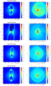 |
Fig. A.1 Density slices perpendicular (left) and parallel to the disk plane (right). First row: FLD method, uniform; second row: hybrid method, uniform; third row: FLD method, peaked; fourth row: hybrid method, peaked. |
References
- Anglada, G., Rodriguez, L. F., Canto, J., Estalella, R., & Torrelles, J. M. 1992, ApJ, 395, 494 [NASA ADS] [CrossRef] [Google Scholar]
- Anglada, G., Rodríguez, L. F., & Carrasco-González, C. 2018, A&ARv, 26, 3 [Google Scholar]
- Arce, H. G., Shepherd, D., Gueth, F., et al. 2007, Protostars and Planets V, eds. B. Reipurth, D. Jewitt, & K. Keil (Tucson: University of Arizona Press), 951, 245 [NASA ADS] [Google Scholar]
- Arce-Tord, C., Louvet, F., Cortes, P. C., et al. 2020, A&A, 640, A111 [NASA ADS] [CrossRef] [EDP Sciences] [Google Scholar]
- Bally, J. 2016, ARA&A, 54, 491 [Google Scholar]
- Banerjee, R., & Pudritz, R. E. 2006, ApJ, 641, 949 [NASA ADS] [CrossRef] [Google Scholar]
- Banerjee, R., & Pudritz, R. E. 2007, ApJ, 660, 479 [NASA ADS] [CrossRef] [Google Scholar]
- Beltrán, M. 2020, Perspective Section of the Star Formation Newsletter, [arXiv:2005.06912] [Google Scholar]
- Beuther, H., Schilke, P., Sridharan, T. K., et al. 2002, A&A, 383, 892 [NASA ADS] [CrossRef] [EDP Sciences] [Google Scholar]
- Blandford, R. D., & Payne, D. G. 1982, MNRAS, 199, 883 [CrossRef] [Google Scholar]
- Bonnell, I. A., Bate, M. R., & Zinnecker, H. 1998, MNRAS, 298, 93 [Google Scholar]
- Cabrit, S., & Bertout, C. 1990, ApJ, 348, 530 [CrossRef] [Google Scholar]
- Cabrit, S., & Bertout, C. 1992, A&A, 261, 274 [Google Scholar]
- Cabrit, S., Edwards, S., Strom, S. E., & Strom, K. M. 1990, ApJ, 354, 687 [Google Scholar]
- Cesaroni, R., Sánchez-Monge, Á., Beltrán, M. T., et al. 2017, A&A, 602, A59 [NASA ADS] [CrossRef] [EDP Sciences] [Google Scholar]
- Chapman, N. L., Davidson, J. A., Goldsmith, P. F., et al. 2013, ApJ, 770, 151 [NASA ADS] [CrossRef] [Google Scholar]
- Ciardi, A., & Hennebelle, P. 2010, MNRAS, 409, L39 [NASA ADS] [Google Scholar]
- Commerçon, B., Hennebelle, P., & Henning, T. 2011, ApJ, 742, L9 [CrossRef] [Google Scholar]
- Commerçon, B., González, M., Mignon-Risse, R., Hennebelle, P., & Vaytet, N. 2021, A&A, submitted [Google Scholar]
- de Valon, A., Dougados, C., Cabrit, S., et al. 2020, A&A, 634, L12 [NASA ADS] [CrossRef] [EDP Sciences] [Google Scholar]
- Fernández-López, M., Curiel, S., Girart, J. M., et al. 2011, ApJ, 141, 72 [CrossRef] [Google Scholar]
- Fernández-López, M., Girart, J. M., Curiel, S., et al. 2013, ApJ, 778, 72 [CrossRef] [Google Scholar]
- Flock, M., Fromang, S., González, M., & Commerçon, B. 2013, A&A, 560, A43 [NASA ADS] [CrossRef] [EDP Sciences] [Google Scholar]
- Fromang, S., Hennebelle, P., & Teyssier, R. 2006, A&A, 457, 371 [NASA ADS] [CrossRef] [EDP Sciences] [Google Scholar]
- Galametz, M., Maury, A., Girart, J. M., et al. 2018, A&A, 616, A139 [NASA ADS] [CrossRef] [EDP Sciences] [Google Scholar]
- Ginsburg, A., Bally, J., Goddi, C., Plambeck, R., & Wright, M. 2018, ApJ, 860, 119 [NASA ADS] [CrossRef] [Google Scholar]
- Girart, J. M., Estalella, R., Fernández-López, M., et al. 2017, ApJ, 847, 58 [CrossRef] [Google Scholar]
- Goddi, C., Ginsburg, A., Maud, L. T., Zhang, Q., & Zapata, L. A. 2020, ApJ, 905, 25 [NASA ADS] [CrossRef] [Google Scholar]
- Gressel, O., Ramsey, J. P., Brinch, C., et al. 2020, ApJ, 896, 126 [Google Scholar]
- Hennebelle, P., & Ciardi, A. 2009, A&A, 506, L29 [NASA ADS] [CrossRef] [EDP Sciences] [Google Scholar]
- Hennebelle, P., & Fromang, S. 2008, A&A, 477, 9 [NASA ADS] [CrossRef] [EDP Sciences] [Google Scholar]
- Hennebelle, P., Commerçon, B., Joos, M., et al. 2011, A&A, 528, A72 [NASA ADS] [CrossRef] [Google Scholar]
- Hirota, T., Machida, M. N., Matsushita, Y., et al. 2017, Nat. Astron., 1, 146 [NASA ADS] [CrossRef] [Google Scholar]
- Hirota, T., Plambeck, R. L., Wright, M. C. H., et al. 2020, ApJ, 896, 157 [NASA ADS] [CrossRef] [Google Scholar]
- Hull, C. L. H., Plambeck, R. L., Bolatto, A. D., et al. 2013, ApJ, 768, 159 [Google Scholar]
- Hull, C. L. H., Plambeck, R. L., Kwon, W., et al. 2014, ApJS, 213, 13 [NASA ADS] [CrossRef] [Google Scholar]
- Joos, M., Hennebelle, P., & Ciardi, A. 2012, A&A, 543, A128 [NASA ADS] [CrossRef] [EDP Sciences] [Google Scholar]
- Joos, M., Hennebelle, P., Ciardi, A., & Fromang, S. 2013, A&A, 554, A17 [NASA ADS] [CrossRef] [EDP Sciences] [Google Scholar]
- Kato, Y., Mineshige, S., & Shibata, K. 2004, ApJ, 605, 307 [NASA ADS] [CrossRef] [Google Scholar]
- Kölligan, A., & Kuiper, R. 2018, A&A, 620, A182 [NASA ADS] [CrossRef] [EDP Sciences] [Google Scholar]
- Krumholz, M. R., & Matzner, C. D. 2009, ApJ, 703, 1352 [NASA ADS] [CrossRef] [Google Scholar]
- Krumholz, M. R., McKee, C. F., & Klein, R. I. 2005, ApJ, 618, L33 [NASA ADS] [CrossRef] [Google Scholar]
- Kuiper, R., & Hosokawa, T. 2018, A&A, 616, A101 [NASA ADS] [CrossRef] [EDP Sciences] [Google Scholar]
- Kuiper, R., & Yorke, H. W. 2013, ApJ, 772, 61 [Google Scholar]
- Kuiper, R., Klahr, H., Dullemond, C., Kley, W., & Henning, T. 2010, A&A, 511, A81 [NASA ADS] [CrossRef] [EDP Sciences] [Google Scholar]
- Kuiper, R., Klahr, H., Beuther, H., & Henning, T. 2011, ApJ, 732, 20 [CrossRef] [Google Scholar]
- Kuiper, R., Klahr, H., Beuther, H., & Henning, T. 2012, A&A, 537, A122 [NASA ADS] [CrossRef] [EDP Sciences] [Google Scholar]
- Kuiper, R., Yorke, H. W., & Turner, N. J. 2015, ApJ, 800, 86 [NASA ADS] [CrossRef] [Google Scholar]
- Lada, C. J. 1985, Ann. Rev. Astron. Astrophys., 23, 267 [CrossRef] [Google Scholar]
- Levermore, C. D. 1984, J. Quant. Spectr. Rad. Transf., 31, 149 [NASA ADS] [CrossRef] [Google Scholar]
- Levermore, C. D., & Pomraning, G. C. 1981, ApJ, 248, 321 [NASA ADS] [CrossRef] [Google Scholar]
- Lynden-Bell, D. 1996, MNRAS, 279, 389 [NASA ADS] [CrossRef] [Google Scholar]
- Lynden-Bell, D. 2003, MNRAS, 341, 1360 [NASA ADS] [CrossRef] [Google Scholar]
- Machida, M. N., & Hosokawa, T. 2020, MNRAS, 499, 4490 [NASA ADS] [CrossRef] [Google Scholar]
- Masson, J., Teyssier, R., Mulet-Marquis, C., Hennebelle, P., & Chabrier, G. 2012, ApJS, 201, 24 [Google Scholar]
- Matsushita, Y., Machida, M. N., Sakurai, Y., & Hosokawa, T. 2017, MNRAS, 470, 1026 [NASA ADS] [CrossRef] [Google Scholar]
- Melon Fuksman, J. D., Klahr, H., Flock, M., & Mignone, A. 2021, ApJ, 906, 78 [NASA ADS] [CrossRef] [Google Scholar]
- Mignon-Risse, R., González, M., Commerçon, B., & Rosdahl, J. 2020, A&A, 635, A42 [NASA ADS] [CrossRef] [EDP Sciences] [Google Scholar]
- Mignon-Risse, R., González, M., Commerçon, B., & Rosdahl, J. 2021, A&A, 652, A69, (Paper I) [NASA ADS] [CrossRef] [EDP Sciences] [Google Scholar]
- Moscadelli, L., Cesaroni, R., & Rioja, M. J. 2005, A&A, 438, 889 [NASA ADS] [CrossRef] [EDP Sciences] [Google Scholar]
- Motte, F., Bontemps, S., & Louvet, F. 2018, ARA&A, 56, 41 [NASA ADS] [CrossRef] [Google Scholar]
- Mouschovias, T. C., & Spitzer, Jr. L. 1976, ApJ, 210, 326 [NASA ADS] [CrossRef] [Google Scholar]
- Nony, T., Motte, F., Louvet, F., et al. 2020, A&A, 636, A38 [NASA ADS] [CrossRef] [EDP Sciences] [Google Scholar]
- Offner, S. S. R., Lee, E. J., Goodman, A. A., & Arce, H. 2011, ApJ, 743, 91 [CrossRef] [Google Scholar]
- Ogilvie, G. I. 2016, J. Plasma Phys., 82, 3 [CrossRef] [Google Scholar]
- Olofsson, S., & Olofsson, G. 2009, A&A, 498, 455 [NASA ADS] [CrossRef] [EDP Sciences] [Google Scholar]
- Owen, J. E., Ercolano, B., & Clarke, C. J. 2014, in The Labyrinth of Star Formation, eds. D. Stamatellos, S. Goodwin, & D. Ward-Thompson (Berlin: Springer), 36, 127 [NASA ADS] [CrossRef] [Google Scholar]
- Pelletier, G., & Pudritz, R. E. 1992, ApJ, 394, 117 [NASA ADS] [CrossRef] [Google Scholar]
- Peretto, N., Fuller, G. A., Duarte-Cabral, A., et al. 2013, A&A, 555, A112 [NASA ADS] [CrossRef] [EDP Sciences] [Google Scholar]
- Peters, T., Banerjee, R., Klessen, R. S., & Low, M.-M. M. 2011, ApJ, 729, 72 [NASA ADS] [CrossRef] [Google Scholar]
- Peters, T., Klaassen, P. D., Seifried, D., Banerjee, R., & Klessen, R. S. 2014, MNRAS, 437, 2901 [NASA ADS] [CrossRef] [Google Scholar]
- Pety, J., Gueth, F., Guilloteau, S., & Dutrey, A. 2006, A&A, 458, 841 [NASA ADS] [CrossRef] [EDP Sciences] [Google Scholar]
- Pudritz, R. E., & Norman, C. A. 1983, ApJ, 274, 677 [NASA ADS] [CrossRef] [Google Scholar]
- Pudritz, R. E., & Ray, T. P. 2019, Front. Astron. Space Sci., 6, 54 [Google Scholar]
- Pudritz, R. E., Ouyed, R., Fendt, C., & Brandenburg, A. 2007, Protostars and Planets V, eds. B. Reipurth, D. Jewitt, & K. Keil (Tucson: University of Arizona Press), 951, 277 [NASA ADS] [Google Scholar]
- Ramsey, J. P., & Dullemond, C. P. 2015, A&A, 574, A81 [NASA ADS] [CrossRef] [EDP Sciences] [Google Scholar]
- Rodriguez, L. F., Garay, G., Brooks, K. J., & Mardones, D. 2005, ApJ, 626, 953 [NASA ADS] [CrossRef] [Google Scholar]
- Rosen, A. L., & Krumholz, M. R. 2020, AJ, 160, 78 [NASA ADS] [CrossRef] [Google Scholar]
- Rosen, A. L., Krumholz, M. R., McKee, C. F., & Klein, R. I. 2016, MNRAS, 463, 2553 [NASA ADS] [CrossRef] [Google Scholar]
- Rosen, A., Krumholz, M., Oishi, J., Lee, A., & Klein, R. 2017, J. Comput. Phys., 330, 924 [NASA ADS] [CrossRef] [Google Scholar]
- Rosen, A. L., Li, P. S., Zhang, Q., & Burkhart, B. 2019, ApJ, 887, 108 [NASA ADS] [CrossRef] [Google Scholar]
- Seifried, D., Pudritz, R. E., Banerjee, R., Duffin, D., & Klessen, R. S. 2012, MNRAS, 422, 347 [NASA ADS] [CrossRef] [Google Scholar]
- Spruit, H. C. 1996, Evolutionary processes in binary stars, NATO ASI Series C (The Netherlands: Kluwer academic publishers), 477, 249 [NASA ADS] [CrossRef] [Google Scholar]
- Teyssier, R. 2002, A&A, 385, 337 [NASA ADS] [CrossRef] [EDP Sciences] [Google Scholar]
- Vaidya, B., Fendt, C., Beuther, H., & Porth, O. 2011, ApJ, 742, 56 [NASA ADS] [CrossRef] [Google Scholar]
- Vaytet, N., Commerçon, B., Masson, J., González, M., & Chabrier, G. 2018, A&A, 615, A5 [NASA ADS] [CrossRef] [EDP Sciences] [Google Scholar]
- Vázquez-Semadeni, E., Gómez, G. C., Jappsen, A.-K., Ballesteros-Paredes, J., & Klessen, R. S. 2009, ApJ, 707, 1023 [CrossRef] [Google Scholar]
- Wu, Y., Wei, Y., Zhao, M., et al. 2004, A&A, 426, 503 [NASA ADS] [CrossRef] [EDP Sciences] [Google Scholar]
- Wu, Y., Zhang, Q., Chen, H., et al. 2005, AJ, 129, 330 [NASA ADS] [CrossRef] [Google Scholar]
- Wurster, J., Bate, M. R., & Bonnell, I. A. 2021, MNRAS, 507, 2354 [NASA ADS] [CrossRef] [Google Scholar]
- Zhang, Q., Hunter, T. R., Brand, J., et al. 2005, ApJ, 625, 864 [NASA ADS] [CrossRef] [Google Scholar]
- Zhang, Y., Arce, H. G., Mardones, D., et al. 2016, ApJ, 832, 158 [NASA ADS] [CrossRef] [Google Scholar]
All Tables
All Figures
|
Fig. 1 Outflow selection slice perpendicular to the disk in run NOTURB, showing three of the eight steps to compute its opening angle. Displayed are the projection vector pi associated to cell i (Eq. (3), left panel), the four subselections based on this projection (middle panel) and the geometric center vector u, and two of the outermost positions vectors r2,± used to compute the opening angle (Eq. (4), right panel). The circle shows the sink position that we consider as the coordinates origin. |
| In the text | |
|
Fig. 2 Slices of 10 000 AU of three forces ratios when M = 10 M⊙ (L = 2 × 10⁴ L⊙) in run NOTURB (top) and when M = 23.8 M⊙ (L = 1.2 × 10⁵ L⊙) in run LRNOTURB. Left panels: Lorentz against gravitational acceleration. Middle panels: Lorentz acceleration against radiative acceleration. Right panels: radiative acceleration against gravitational acceleration. Lorentz acceleration dominates over the radiative acceleration everywhere but close to the protostar. |
| In the text | |
|
Fig. 3 Slice of 1000 AU showing the ratio of the FLD radiative acceleration to the gravitational acceleration (top) and to the M1 radiative acceleration (bottom), perpendicular to the disk plane in run NOTURB, when M = 12.7 M⊙. Below M = 10 M⊙, the FLD radiative acceleration rarely dominates the gravitational acceleration. The M1 acceleration dominates in the outflow region over the FLD acceleration and the disk region is dominated by the FLD acceleration. |
| In the text | |
|
Fig. 4 Gas density slice of 20000 AU in the outflow selection perpendicular to the disk plane: run NOTURB, M = 10 M⊙. The gas outflow density corresponds to particle densities between ~105 cm−3 and ~ 107 cm−3. |
| In the text | |
|
Fig. 5 Gas density slice of 500 AU perpendicular to the disk plane: run NOTURB, M = 10 M⊙. Velocity vectors and magnetic lines are overplotted. The gas density corresponds to particle densities between ~ 106 and ~ 1013 cm−3. |
| In the text | |
|
Fig. 6 Left panel: ratio of the magnetic-pressure-gradient acceleration and the gravitational acceleration in the vertical direction. Right panel: ratio of the poloidal and toroidal components of the magnetic field and velocity vectors overplotted. Slices of 20 000 AU perpendicular to the disk plane are shown, when M = 10 M⊙; run NOTURB. |
| In the text | |
|
Fig. 7 Plasma β and Lorentz acceleration vectors overplotted. Slice of 20 000 AU perpendicular to the disk plane, when M = 10 M⊙, run NOTURB. |
| In the text | |
|
Fig. 8 Criterion for centrifugal acceleration (Eq. (7)) from Seifried et al. (2012) applied to a slice of 4000 AU perpendicular to the disk plane. Run NOTURB, M = 10 M⊙. Red regions are consistent with centrifugal acceleration. |
| In the text | |
|
Fig. 9 Poloidal velocity as a function of the distance to the sink (mainly in the vertical direction), in a cylindrical selection of cells with rcyl < 100 AU. Negative radial velocities have been masked out. Velocities are obtained as averages over a distance bin. A and B label the northern and southern outflow, respectively, and the vertical lines indicate the positions where the poloidal velocity equals the Alfvén poloidal velocity (averaged over the same distance bin). Run NOTURB, M = 10 M⊙. |
| In the text | |
|
Fig. 10 Slices perpendicular to the disk plane. Left column: density slice in the outflow selection. Middle column: ratio of the Lorentz acceleration to the radiative acceleration. Right column: ratio of the radiative acceleration to the gravitational force. From top to bottom: Run SUPA (super-Alfvénic, subsonic turbulence, 10 000 AU, t = 67.0 kyr, M = 8.2 M⊙, L = 1.4 × 10⁴ L⊙), run SUPAS (super-Alfvénic, supersonic turbulence, 4000 AU, t = 72.6 kyr, M = 5.6 M⊙, L = 8 × 10³ L⊙) and run SUBA (sub-Alfvénic, subsonic turbulence, 10 000 AU, t = 61.1 kyr, M = 9.6 M⊙, L = 1.7 × 10⁴ L⊙). The gas densities in the left column correspond to particle densities between ~ 104 and ~ 106 cm−3. |
| In the text | |
|
Fig. 11 Ratio between the radiative and Lorentz accelerations (both integrated over the outflow volume) as a function of the sink luminosity. |
| In the text | |
|
Fig. 12 Outflow mass as a function of the sink mass. |
| In the text | |
|
Fig. 13 Outflow properties as a function of the primary sink age: momentum rate (left), maximal outflow radius (middle), opening angle (right), and angle between the outflow and the large-scale magnetic field (bottom-right), in runs NOTURB, SUPA, SUBA. Forces and opening angles of outflows composed of less than 50 cells are not displayed. Outflows come in pairs in these runs, so they are individually labeled as A and B. Values are averaged over 0.5 kyr (smaller than the orbital timescale in run SUPA). |
| In the text | |
|
Fig. 14 Angle between the outflow and the large-scale magnetic field (left), the core-scale angular momentum (middle), and the disk (right), respectively, in runs NOTURB, SUPA, SUBA. Values obtained for outflows composed of less than 50 cells are notdisplayed. Outflows come in pairs in these runs, so they are individually labeled as A and B. |
| In the text | |
|
Fig. A.1 Density slices perpendicular (left) and parallel to the disk plane (right). First row: FLD method, uniform; second row: hybrid method, uniform; third row: FLD method, peaked; fourth row: hybrid method, peaked. |
| In the text | |
Current usage metrics show cumulative count of Article Views (full-text article views including HTML views, PDF and ePub downloads, according to the available data) and Abstracts Views on Vision4Press platform.
Data correspond to usage on the plateform after 2015. The current usage metrics is available 48-96 hours after online publication and is updated daily on week days.
Initial download of the metrics may take a while.