| Issue |
A&A
Volume 634, February 2020
|
|
|---|---|---|
| Article Number | A124 | |
| Number of page(s) | 10 | |
| Section | Galactic structure, stellar clusters and populations | |
| DOI | https://doi.org/10.1051/0004-6361/201937284 | |
| Published online | 20 February 2020 | |
The strange case of the peculiar spiral galaxy NGC 5474
New pieces of a galactic puzzle
1
INAF – Osservatorio di Astrofisica e Scienza dello Spazio di Bologna, Via Gobetti 93/3, 40129 Bologna, Italy
e-mail: This email address is being protected from spambots. You need JavaScript enabled to view it.
2
Dipartimento di Fisica e Astronomia, Università degli Studi di Bologna, Via Gobetti93/2, 40129 Bologna, Italy
3
Dipartimento di Fisica, Università of Pisa, Largo B. Pontecorvo 3, 56127 Pisa, Italy
4
European Southern Observatory, Karl-Schwarzschild-Strasse 2, 85748 Garching bei München, Germany
Received:
9
December
2019
Accepted:
7
January
2020
Abstract
We present the first analysis of the stellar content of the structures and substructures identified in the peculiar star-forming galaxy NGC 5474, based on Hubble Space Telescope resolved photometry from the LEGUS survey. NGC 5474 is a satellite of the giant spiral M 101, and it is known to have a prominent bulge that is significantly off-set from the kinematic centre of the underlying H I and stellar disc. The youngest stars (age ≲ 100 Myr) trace a flocculent spiral pattern extending out to ≳8 kpc from the centre of the galaxy. On the other hand, intermediate-age (age ≳ 500 Myr) and old (age ≳ 2 Gyr) stars dominate the off-centred bulge and a large substructure residing in the south-western part of the disc (SW over-density) and they are not correlated with the spiral arms. The old age of the stars in the SW over-density suggests that this may be another signature of any dynamical interactions that have shaped this anomalous galaxy. We suggest that a fly by with M 101, generally invoked as the origin of the anomalies, may not be sufficient to explain all the observations. A more local and more recent interaction may help to put all the pieces of this galactic puzzle together.
Key words: galaxies: individual: NGC 5474 / galaxies: peculiar / galaxies: interactions / galaxies: stellar content / galaxies: structure
© ESO 2020
1. Introduction
NGC 54741 is a satellite of M 101 (the Pinwheel galaxy) classified as SAcd pec. It is located at 6.98 Mpc from us (Tully et al. 2013) in the M 101 group (Tully et al. 2016) at 0.74° from the centre of M 101, corresponding to ≃90 kpc in projection and 0.80° from NGC 5477, another member of the group. Its absolute integrated visual magnitude, MV ≃ −18.5, is ≃1.5 mag brighter than the conventional limit for dwarf galaxies, which was adopted, for example, by Tolstoy et al. (2009). The total visual luminosity of NGC 5474 is about 1.5 times that of the Large Magellanic Cloud (McConnachie 2012).
The most obvious reason for it being classified as peculiar is readily visible in the image shown in Fig. 1, where a seemingly circular compact bulge (hereafter “the bulge”, for brevity) is clearly seen to lie at the northern edge of what appears as a bright, nearly face-on, stellar disc. Moreover any additional piece of observational evidence seems to add more complexity to the overall picture of this system (see, e.g, Rownd et al. 1994; Gonzàlez Delgado et al. 1997; Kornreich et al. 1998, 2000; Epinat et al. 2008; Mihos et al. 2013, for discussion and references).
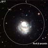 |
Fig. 1. RGB colour image of NGC 5474 obtained with SDSS images in g, r, and i band, for the blue, green, and red channels, respectively. North is up and east is to the left. The white circle is centred on the centre of the bulge. |
The three panels of Fig. 2, showing images of the galaxy at different wavelengths, provide the basis for a more thorough illustration of most of the anomalies affecting NGC 5474. In the central panel, we marked and labelled some remarkable features, for reference. In particular, the small red circle marks the optical centre of the bulge, which is easy to locate (see, e.g. the intensity contours in Fig. 5, below) and coincides with the position of a nuclear star cluster (see Sect. 2.2). The large red circle has a radius of R = 30.0″ (corresponding to r ≃ 1.0 kpc, at the distance of NGC 5474) and encloses the entirety of the optical bulge. The small cyan square marks the position of the kinematic centre of the H I disc, as determined by Rownd et al. (1994, R94, hereafter) and confirmed by Kornreich et al. (2000, K00, hereafter). It is worth noting that while the Hα velocity field is compatible with having the same kinematic centre as the H I, the amplitude of the Hα rotation curve seems to be significantly larger (Vmax sin (i)≃25 km s−1 vs. Vmax sin (i)≃8 km s−1; Epinat et al. 2008; Kornreich et al. 2000). Finally, the large blue circle is centred on the kinematic centre of the disc and has a radius of R = 240.0″, corresponding to r ≃ 8.1 kpc. Kornreich et al. (2000) traced the H I disc out to R ≃ 400″, corresponding to r ≃ 13.5 kpc. It is apparent from the Galaxy Evolution Explorer (GALEX) far ultraviolet (FUV) and Hα images of Fig. 2 that the youngest stars follow an irregular but clear and wide spiral pattern, whose centre of symmetry roughly coincides with the kinematic centre of the disc. However the strongest ultraviolet (UV) emission and some of the most remarkable H II regions are clustered in a bar-like structure that overlaps the bulge. Moreover the i-band image reveals the presence of a significant stellar over-density to the south-west of the bulge, with the shape of a fat crescent (SW over-density, see also Fig. 1). The latter feature does not coincide with the spiral arms, but it seems to match the position of a local minimum in the H I distribution (see Fig. 9 by K00). The sub-structure is approximately comprised in the range of angular distances from the centre of the bulge 50.0″ ≲ R ≲ 110.0″ (corresponding to the range 1.7 kpc to 3.7 kpc), with a surface density peak at R ≃ 65″ ≃ 2.2 kpc. It is interesting to note that the bulge does not seem strikingly off-set with respect to the overall spiral pattern. The strong displacement is with the kinematic centre of the H I distribution, and with the structure that, for historical reasons, we refer to as the “bright disc” (we use this name again in the following, for brevity). This is in fact a nearly circular cloud of redder light, which is seen in i-band but not in FUV, that encloses and surrounds the SW over-density.
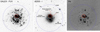 |
Fig. 2. Images of NGC 5474 at different wavelengths. Left: GALEX-FUV, centre: SDSS-i, Right: continuum-subtracted Hα image (retrieved from NED, where it is attributed to Dale et al. 2009). All the images have the same scale and are aligned. The small red circle is the photometric centre of the bulge, the wide red circle has radius = 30.0″ and encloses the bulge, the small cyan square is the kinematic centre of the H I disc (according to Rownd et al. 1994), and the wide blue circle is centred on this point and has a radius = 240.0″. North is up and east is to the left. |
Both R94 and K00 find that the H I disc displays a very regular velocity field in the central region, while beyond ≃180″ from the kinematic centre the typical features of a strongly warped disc become apparent, with the orientation of the kinematic major axis of the cold gas changing by more than 50°. The disc of the galaxy is nearly face-on with respect to the line of sight (i = 21°; Kornreich et al. 2000); this makes the derivation of the true amplitude of the rotation curve and, consequently, the estimates of the total dynamical mass are especially uncertain (Mdyn = 2−6.5 × 10⁹ M⊙; Rownd et al. 1994).
The various dynamical disturbances observed in NGC 5474 are generally attributed to its interaction with M 101, which also displays signs of interaction with the environment (see, e.g. Mihos et al. 2013) and is connected to NGC 5474 by a bridge of H I clouds and filaments (Hutchmeier & Witzel 1979; Mihos et al. 2012). However, as far as we know, a quantitative modelling of the interaction has never been attempted.
Here we present the results of the analysis of the deep photometry of individual stars in NGC 5474, which were obtained and made publicly available by the LEGUS collaboration (Calzetti et al. 2015; Sabbi et al. 2018) from Hubble Space Telescope (HST) optical (F606W, F814W) images acquired with the Wide Field Channel (WFC) of the Advanced Camera for Surveys (ACS). In particular, for the first time, we reveal the stellar content of the various asymmetric components of the galaxy, providing new observational insight into their possible origin. This study is part of an ongoing broader project aimed at searching for the observational signatures of the process of hierarchical merging in dwarf galaxies, the Smallest Scale of Hierarchy Survey (SSH) survey (Annibali et al. 2019).
Throughout the paper we adopt (m − M)0 = 29.22 ± 0.20, corresponding to D = 6.98 Mpc from Tully et al. (2013), and a foreground extinction of AV = 0.029 from the NASA/IPAC Extragalactic Database (NED), which is in good agreement with Gil de Paz et al. (2007). For the present-day oxygen abundance, we assume 12 + log(O/H) = 8.31 ± 0.22, which was estimated in H II regions by Moustakas et al. (2011) with the calibration by Pilyugin & Thuan (2005), corresponding to [M/H] ≃ −0.4 and Z ≃ 0.006.
The outline of the paper is the following: in Sect. 2 we present newly derived light profiles of the bulge and of the nuclear star cluster; in Sect. 3 we present the colour-magnitude diagram and the spatial distribution of stars as a function of their age. Finally, in Sect. 4 we discuss the main results of the analysis.
2. Surface photometry
2.1. The bulge
To obtain structural parameters and estimate the stellar mass of the bulge, we followed the same approach adopted by Bellazzini et al. (2017), using r and i band images from the Sloan Digital Sky Survey (SDSS) DR12 (Alam et al. 2015). These sky-subtracted images are flux-calibrated in nMgy units2, which can be easily converted into AB magnitudes with the relation mag = −2.5log(F[nMgy] + 22.5).
First, we determined the centre of the bulge as the position of the highest intensity peak on the image, with the aid of density contours. Then, the Aperture Photomety Tool software (APT, Laher et al. 2012) was used to perform surface photometry. We derived the surface brightness profile over a series of concentric circular apertures covering the whole extension of the bulge, up to 33.5″. To remove the contribution of the underlying disc, we estimated the background in a concentric annulus sampling that component and we subtracted it from the fluxes within the apertures. The background-subtracted surface brightness profile is shown in Fig. 3. All the parameters derived from the surface photometry are listed in Table 1. We used the i band as a reference for the profile and for estimating the stellar mass because in this band the light contribution from young stars, which is presumably unrelated to the bulge, should be minimal.
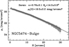 |
Fig. 3. Surface brightness profile of the bulge of NGC 5474 in the SDSS i band. The continuous line is the Sérsic model that best-fits the observed profile. |
Properties of the bulge of NGC 5474.
The parameters of the best-fit Sérsic model (Sérsic 1968)3, which are listed in Table 1, are in good agreement with those obtained by Fisher & Drory (2010) from 3.6 μm band images from the Spitzer space mission once the difference in the assumed distance are taken into account (n = 0.74 ± 0.2 and re = 439 ± 100 pc, corrected to our distance). The structural parameters of the bulge of NGC 5474 are consistent with those of pseudo-bulges (Kormendy & Kennicutt 2004; Fisher & Drory 2008), and indeed it is classified as such by Fisher & Drory (2010). It is interesting to note that these parameters are also fully compatible with the scaling laws of dwarf galaxies (see, e.g. Côté et al. 2008; Lange et al. 2015; Bellazzini et al. 2017; Marchi-Lasch et al. 2019). In particular, the absolute integrated magnitude, the stellar mass, and the effective radius of the bulge are quite similar to those of NGC 205, a nucleated dwarf elliptical satellite of M 31 (MV = −16.5 ± 0.1, M⋆ = 3.3 × 10⁸ M⊙, assuming M/LV = 1.0, and Re = 445 ± 25 pc (circularised), from McConnachie 2012).
2.2. The stellar nucleus
The inspection of the ACS images has revealed the presence of a star cluster residing at the centre of the bulge (see the upper panel of Fig. 4). The object is not resolved into stars but it is clearly more extended than the stellar point spread function (PSF).
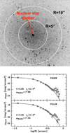 |
Fig. 4. Upper panel: HST ACS F814W zoomed image of the central part of the bulge with intensity cuts chosen to make the stellar nucleus visible. The concentric circles provide the scale of the image and help the eye to appreciate that the nucleus resides at the centre of the bulge. Lower panel: surface brightness profile of the stellar nucleus in both the ACS bands. The continuous line displays the King (1966) model that fits the observed profiles. The parameters of the model are reported in the panels. The deviation from a smooth profile observed around log(R) = 0.75 is due to a relatively bright source projected onto the outskirts of the nucleus. |
In the lower panels of Fig. 4, we show the surface brightness profile of the stellar nucleus obtained with APT aperture photometry on concentric circular annuli as mentioned above from the F606W and F814W ACS images. The profiles are nicely fitted by a King (1966) model with a concentration of C = 0.90 and a core radius of rc = 0.14″. The theoretical profile has been convolved with a Gaussian distribution with FWHM = 0.1″ to account for the smoothing due to the HST PSF. These and other measured properties of the system are listed in Table 2. The structural properties of the stellar nucleus derived here are in reasonable agreement with those provided by Georgiev & Böker (2014), who include it among those surveyed in their sample of 228 spiral galaxies.
Properties of the nuclear star cluster of NGC 5474.
The nuclear cluster has a stellar mass typical of globular clusters (GCs) and a (V − I)0 colour compatible with the most metal-poor Galactic GCs (Smith & Strader 2007). It fits well with the relation between rh and C of Galactic globular clusters (GGC, Djorgovski et al. 2003), but its concentration parameter is lower than any GGC with a similar MV (Djorgovski & Meylan 1994). The ratio of its stellar mass to that of the bulge as a whole obeys the relation that is known to exist between the stellar masses of galaxies and of their nuclei (see, e.g. Sánchez-Janssen et al. 2018, and references therein). The presence of a nuclear star cluster is a further element of similarity with NGC 205 (see, e.g. Heat et al. 1996, and references therein); the colour of the nuclei are also similar (Nguyen et al. 2019).
3. Photometry of resolved stars
We retrieved4 the F606W and F814W photometric catalogues produced by LEGUS (Calzetti et al. 2015) from ACS images that are nearly centred on the bulge of NGC 5474. The F814W drizzled image at the origin of this dataset is shown if Fig. 5. In this figure the intensity contours highlight the bulge and the SW over-density very clearly. All the details on the data reduction and on the parameters included in the catalogues are reported in Sabbi et al. (2018).
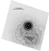 |
Fig. 5. HST ACS drizzled image of NGC 5474 in the F814W filter. The intensity contours are at 0.04, 0.08, 0.12, 0.25, 0.5, 1.0, and 2.0 e− s−1. The black circle marks the position of the kinematic centre of the H I disc. |
First, we selected from each catalogue only the sources classified as bona fide stars, then we applied further selections based on various quality parameters. In particular, we required that stars that were retained in the final catalogues satisfy the following conditions: ROUND < 3.0, CHISQ < 2.0, |SHARP| < 0.2, and CROWD < 0.2, for both F606W and F814W (see Sabbi et al. 2018, for the meaning of the parameters). We matched the two catalogues using CataXcorr5 with a first degree transformation, ending up with a merged catalogue with 137174 stars. Finally, we added to our catalogue V, I magnitudes in the Johnson-Cousins system, which were obtained from F606W and F814W magnitudes with the transformations by Harris (2018).
We transferred to the catalogue the astrometry embedded in the drizzled images provided by LEGUS. This was done by reducing the F606W image with Sextractor (Bertin & Arnouts 1996), with a 10σ detection threshold, in order to obtain an output catalogue with positions in RA and Dec. Then we used CataXcorr to cross-correlate this catalogue with the catalogue we got from LEGUS, and we transformed pixel coordinates into equatorial coordinates with a first degree polynomial in x,y fitted on 32571 stars in common, which are well distributed over the whole field. The residual of the transformation are < 0.2″ in both coordinates. The astrometric solution embedded in drizzled images may have a small zero-point residual. We checked with external catalogues and we conclude that the residual should be ≲1.0″, which is negligible for the purposes of the following analysis.
3.1. The colour-magnitude diagram
The upper panel of Fig. 6 shows the colour-magnitude diagram (CMD) of the entire sample of selected stars in the ACS field, which are colour coded according to the square root of the local density. Most of the stars are tightly clustered into a well defined red giant branch (RGB), running from F606W–F814W ≃ 0.5 at F814W ≃ 27.0 to a clear tip located at F814W ≃ 25.1 and ⟨F606W − F814W⟩≃1.1. Stars in this evolutionary phase are older than 1−2 Gyr, and possibly as old as > 10 Gyr. Above the RGB tip, a broad sequence of bright stars bends to the red and culminates at F814W ∼ 24.3. These are asymptotic giant branch (AGB) stars, tracing intermediate to old age populations (age ≳ 100 Myr). The blue vertical plume at F606W–F814W ≲ 0.3 hosts both main sequence stars and stars at the blue edge of the core helium burning phase. The thin diagonal sequence, emerging at the RGB tip level to the blue of the RGB and AGB sequences and running up to F814W ≃ 20.0 at F606W–F814W ≃ 1.3 (red plume), collects stars located at the red edge of the core helium burning phase. All the stars lying in the blue and red plumes and between them are younger than a few ≃100 Myr.
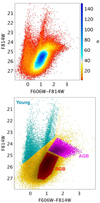 |
Fig. 6. Upper panel: CMD from the HST catalogue. Lower panel: CMD illustrating the boxes adopted to select the various populations. |
In the lower panel of Fig. 6, we illustrate the selection boxes we adopt to trace stellar populations in different age ranges: RGB, AGB, and young stars from both the blue and red plumes. A comparison with theoretical isochrones from the PARSEC set (Marigo et al. 2017) allows for a better age bracketing of the stars enclosed in our selection boxes, which also takes the effect of metallicity into account. In particular, by using isochrones with metallicity corresponding to the oxygen abundance measured in the disc of NGC 5474 (Z = 0.006), we find that our young selection box is only populated by stars that are younger than 100 Myr. The sharp break in the distribution of AGB stars at F814W ∼ 24.3 is matched by isochrones of an age ≳ 630 Myr, for Z = 0.006, and of an age ≳ 1.0 Gyr for Z = 0.0006. Stars that are significantly more metal-poor than the present day metallicity are likely part of the stellar mix when old-intermediate age populations are considered. We conclude that our AGB box includes stars in the age range from ≃0.5 Gyr to 4−5 Gyr, since, according to the adopted stellar evolution models, older age AGB stars in this range of metallicity do not become brighter than the RGB tip. Finally, under the same assumptions, selected RGB stars should have ages in the range ≃2.5 Gyr to ≃12.5 Gyr. In the following section we show and discuss the radial distribution of the various tracers.
In Fig. 7, we show the CMD for different radial annuli centred on the photometric centre of the bulge. This figure illustrates the strong impact of radially varying incompleteness in the region enclosing the bulge (R < 30.0″), with the limiting magnitude dropping from F814W ≃ 27.0 for R ≳ 30.0″ to F814W ≃ 25.5 for R < 10.0″. In the innermost annuli, we notice the smearing of the main CMD features due to the effects of stellar blending and to the increased photometric uncertainty related to the extreme degree of crowding in the bulge region. Outside R = 30.0″, the quality and completeness of the photometry is nearly constant. Figure 7 also shows that the same evolutionary sequences are present everywhere in the considered field, albeit not necessarily with the same relative abundance. The two outermost annuli have been split into their southern and nothern halves (SH and NH, respectively). In these radial ranges (R ≳ 50.0″), the “bright disc” and, in particular, the SW over-density are completely included in the SH, while the NH lack any obvious structure (see Fig. 5; in particular the densest part of SW is included in the SH annulus 50″ ≲ R ≲ 80.0″). This difference is clearly reflected in the corresponding CMDs. However, despite the strong asymmetry in favour of the SH annuli, a significant number of stars associated to NGC 5474 are present in the NH and also in the outermost regions for R ≳ 80.0″. Hence, an extended distribution of intermediate age and old stars, perhaps a halo component, is present everywhere in the sampled field.
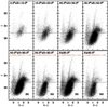 |
Fig. 7. CMD in different radial annuli, from the centre of the bulge to the edge of the ACS image. For R ≳ 50.0″ we split the annuli in their northern and southern halves (NH and SH, respectively) in order to highlight the asymmetry in the surface density related to the SW over-density. In the corresponding panels, we also report the ratio between AGB and RGB stars. The horizontal grey line marks the position of the RGB tip as determined from the whole sample. This series of CMDs also clearly illustrate the severe effect of the increasing incompleteness towards the centre of the most crowded substructure, i.e. the bulge, with the limiting magnitude dropping by nearly 2 mag from R > 30.0″ to R < 10.0″. |
It is interesting to note that the ratio of the number of AGB and RGB stars is significantly larger in SH than in NH, suggesting that intermediate age stars represent a larger fraction of the old and intermediate age population in the region to the south of the bulge that is dominated by the SW over-density, as opposed to the “empty” region to the north of it. While the actual values of this ratio are affected by the incompleteness of the RGB sample, which reaches the limiting magnitude of the photometry, this should equally affect the northern and southern halves of the same radial annulus, thus making the comparison between the ratios in SH and NH meaningful. We verified that the reported differences are unchanged if only RGB stars brighter than I = 26.0 are used, a subset much less affected by incompleteness.
3.2. The spatial distribution of stars
The density maps of the stars belonging to the CMD selection boxes described above are shown in Figs. 8–10, for the YOUNG, the AGB, and the RGB samples, respectively. The positions of the photometric centre of the bulge and of the kinematic centre of the H I disc are reported in all the maps (upper and lower asterisk, respectively).
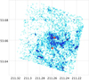 |
Fig. 8. Density map of the YOUNG sample obtained with TOPCAT. The axis are RA and Dec (in degrees) in sin projection. North is up and east is to the left. The colour is proportional to the square root of the local density; darker tones of blue traces higher density levels. The two asterisk symbols superimposed on the map mark the position of the centre of the bulge and of the dynamical centre of the H I disc (from Rownd et al. 1994), from north to south, respectively. |
The stars younger than ≃100 Myr (YOUNG) clearly display the same spiral pattern shown in the left panel of Fig. 2, including the central bar-like structure (see also Cignoni et al. 2019, for an analysis of the youngest stars). While the pattern is visible over the whole field, the densest clusters of young stars lie in the south-west half, also showing that the recent star formation has been asymmetric on large scales (a few kpc).
The intermediate-age AGB stars have a very different distribution. The bulge and the SW over-density stand out as the most remarkable structures, which are possibly connected by a fainter bridge of stars protruding from the eastern edge of the over-density approximately towards the east and reaching the eastern edge of the bulge, after a strong bending towards the north-west.
The map of old RGB stars (Fig. 10) displays a density minimum at the position of the bulge. We should emphasise, however, that the lack of RGB stars in the central bulge is entirely due to the strong incompleteness affecting this region (see Sect. 3) and thus preventing the detection of stars fainter than the AGB. However, the CMD of the outer corona of the bulge (Fig. 7) strongly suggest that RGB stars are an important component of the bulge, albeit unresolved near the centre. On the other hand, the SW over-density and the stellar bridge identified on the AGB map are also quite evident in this map. Hence, we conclude that old and intermediate-age stars trace the SW over-density and dominate its stellar content. On the other hand, Fig. 11, where the density map of the YOUNG stars is superimposed to that of RGB stars, shows that the main spiral arms and the SW over-density are not spatially correlated.
4. Discussion and conclusions
Large asymmetries in the distribution of stars in a galaxy such as NGC 5474 can only be produced by (a) inherently asymmetric star formation episodes, which are quite frequent in star-forming galaxies, or by (b) a strong dynamical disturbance due to an interaction with another galaxy. The old age (> 2 Gyr) of the stars populating the SW over-density militates against the first hypothesis, as orbital mixing should wipe out an over-density originated by an asymmetric episode of star formation within the disc of NGC 5474 in a few orbital times. However, this possibility cannot be completely dismissed since the SW over-density lies in the rising branch of the rotation curve, the rise is approximately solid body (Epinat et al. 2008) and the orbital periods at the relevant distances from the H I kinematic centre are relatively long (in the range 200−400 Myr assuming the Epinat et al. 2008 velocity curve, and > 500 Myr adopting the curve by Kornreich et al. 2000).
A major episode of star formation producing such a conspicuous and long-lasting substructure may have also been triggered by dynamical interaction, the generally hypothesised past encounter with M 101 being the most obvious candidate. However, by assuming that the difference in transverse velocity between M 101 and NGC 5474 is as large as 300 km s−1 (about six times the difference in radial velocity) and that the projected separation (90 kpc) corresponds to the 3D mutual distance, the close encounter with M 101 should have occurred ∼300 Myr ago. Whereas, the hypothetic burst started more than 2 Gyr ago.
In conclusion the variety of anomalies observed in NGC 5474 suggests that it is advisable to also consider the possibility that, in addition to the interaction with M 101, the galaxy also bears the signs of a recent interaction with a dwarf companion. For instance, the SW over-density could be the remnant of a recently disrupted satellite, whose merging triggered the observed enhancement in the recent star formation in the southern half of the gaseous disc. Alternatively, it can be the density wake produced by the off-set of the bulge within the disc or by the passage of a companion. Long-lasting (up to ≃1 Gyr) spiral patterns induced by impulsive interactions have been observed in N-body simulation of galaxy encounters (see, e.g. Struck et al. 2011, and references therein). Still, at least in the cases explored by Struck et al. (2011), they show up as two-arms spiral patterns in stars and gas, which do not seem to match the distribution of old and intermediate-age stars shown in Figs. 9 and 10.
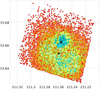 |
Fig. 9. Same as Fig. 8, but for the AGB sample. Here the colour code goes from warm colours (low density) to cold colours (high density). |
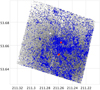 |
Fig. 11. Stars of the YOUNG sample (in blue) are superposed to stars of the RGB sample (in grey) in a map with the same arrangement and symbols as in Fig. 10. |
A natural candidate as a still-alive companion is the putative bulge, a hypothesis already mentioned by other authors (e.g. Mihos et al. 2013). Indeed, Mihos et al. (2013) conclude that the relatively regular outer isophotes of the galaxy are not easy to reconcile with a strong tidal interaction, for example, with a massive galaxy such as M 101, and that the off-centred position of the bulge is suggestive of a recent or on-going interaction with a less conspicuous body.
Some broad consistency check of this hypothesis can be attained, based on the structural similarity of the bulge with local dwarfs (Sect. 2). The latter obey to a tight relation between MV and dynamical mass Mdyn, or, equivalently, the dynamical mass-to-light ratio Mdyn/L, with Mdyn/L in solar units ranging from ∼1000 for the faintest dwarfs to ∼1−3 for the brightest ones, with luminosities similar to the bulge of NGC 5474 (where all the masses and mass-to-light ratios are computed within the half light radius, McConnachie 2012). According to this author, the local galaxy that is more similar to it, NGC 205 (see Sect. 2), has Mdyn/L ≃ Mdyn/Mstar ≃ 2. If we adopt the same for the bulge as a whole, we obtain Mdyn ∼ 8 × 10⁸M⊙, a factor of ∼2.5−8 lower than the dynamical mass of NGC 5474, as estimated from the rotation curve of its gaseous disc (2.0−6.5 × 10⁹M⊙, within 8.8 kpc from the centre; Rownd et al. 1994). A mass ratio ∼0.1−0.2 would probably be broadly consistent with visible but not destructive effects of the encounter. In this case, NGC 5474 would be a bulge-less disc galaxy with a minor stellar halo component and a dynamical mass-to-light ratio of (M/Li)dyn ∼ 20−60. At a first glance, and given the available data, this scenario looks plausible, or it at least merits further analysis.
If the off-set bulge is not actually a bulge, but instead an early-type satellite orbiting around the disc of NGC 5474, then it should have a systemic line-of-sight velocity that is slightly different from that of the disc at the same location. If the hypothetic pair is bound, the difference in the systemic velocity along the line of sight should amount to a few tens of km s−1 at most. Unfortunately the available stellar velocity fields, or individual long slit measures, are all based on emission lines that trace the kinematics of the star-forming disc, which are also in the central regions (Ho et al. 1995; Moustakas et al. 2011; Epinat et al. 2008). On the other hand, the bulge is dominated by old and intermediate-age stars, hence its kinematics can only be traced with absorption line spectra, which are missing6. In principle, one can obtain a spectrum of the bulge region, including both emission lines (from the disc) and absorption lines (from the bulge), and check if the radial velocity of the two components is the same or not.
We did try to perform this test thanks to one night of director discretionary time kindly made available at the 3.5 m Telescopio Nazionale Galileo (TNG) in La Palma. Unfortunately the quality of the data and the reliability of their wavelength calibration were not sufficient to reach our scientific goal (see Appendix A for a description of the encountered problems). The only conclusion that we can draw from the analysis of the acquired spectra is that the radial velocity difference between emission and absorption lines within the bulge is ≲50 km s−1, thus leaving the key question on the nature of the bulge unanswered. However both the limit in the velocity difference between the disc and the bulge and the similarity of the CMD of the two components, indicating similar distances, rules out the hypothesis of the chance superposition of unrelated systems, which was suggested by Rownd et al. (1994), for example.
In summary, the present analysis provides an important piece of information that was lacking from the overall picture of this highly disturbed galaxy, that is the actual stellar content and age distribution of the various and structures and substructures. This is an important element to set the scene for a serious attempt to reproduce the main properties of NGC 5474 with dynamical, and/or hydrodynamical, simulations, which is a task that we are planning for the near future.
Also known as UGC 9013 and VV344b, where VV344a is M 101.
Nanomaggies, see https://www.sdss.org/dr12/algorithms/magnitudes/
We adopt the formulation by Ciotti & Bertin (1999),  , where Re is the 2D half-light radius and bn was computed following Prugniel & Simien (1997).
From the LEGUS website https://legus.stsci.edu
Stellar velocity fields from both emission and absorption lines may possibly be obtained from the data described in (Rosales-Ortega et al. 2010, PINGS project). However, the results for NGC 5474 have been not presented yet.
Acknowledgments
We are grateful to the Referee, Curtis Struck, for a very careful reading of the manuscript and for the useful suggestions for the next steps of the analysis of the NGC 5474 + M 101 system. This research is partially funded through the INAF Main Stream program “SSH” 1.05.01.86.28. F. A., M. C. and M. T. acknowledge funding from INAF PRIN-SKA-2017 program 1.05.01.88.04. Based on observations made with the NASA/ESA Hubble Space Telescope, obtained at the Space Telescope Science Institute, which is operated by the Association of Universities for Research in Astronomy, under NASA Contract NAS 5-26555. These observations are associated with Program 13364. Based on observations made with the Italian Telescopio Nazionale Galileo (TNG) operated on the island of La Palma by the Fundacin Galileo Galilei of the INAF (Istituto Nazionale di Astrofisica) at the Spanish Observatorio del Roque de los Muchachos of the “Instituto de Astrofisica de Canarias”. We are grateful to the TNG staff for their support in preparing the observations. Special thanks are due to the TNG Director Ennio Poretti, to Walter Boschin, Antonio Magazzù and Luca Di Fabrizio. This research made use of SDSS data. Funding for the SDSS and SDSS- II has been provided by the Alfred P. Sloan Foundation, the Participating Institutions, the National Science Foundation, the US Department of Energy, the National Aeronautics and Space Administration, the Japanese Monbukagakusho, the Max Planck Society, and the Higher Education Funding Council for England. The SDSS Website is http://www.sdss.org. The SDSS is managed by the Astrophysical Research Consortium for the Participating Institutions. The Participating Institutions are the American Museum of Natural History, Astrophysical Institute Potsdam, University of Basel, University of Cambridge, Case Western Reserve University, University of Chicago, Drexel University, Fermilab, the Institute for Advanced Study, the Japan Participation Group, Johns Hopkins University, the Joint Institute for Nuclear Astrophysics, the Kavli Institute for Particle Astrophysics and Cosmology, the Korean Scientist Group, the Chinese Academy of Sciences (LAMOST), Los Alamos National Laboratory, the Max-Planck-Institute for Astronomy (MPIA), the Max-Planck- Institute for Astrophysics (MPA), New Mexico State University, Ohio State University, University of Pittsburgh, University of Portsmouth, Princeton University, the United States Naval Observatory, and the University of Washington. Most of the analysis presented in this paper has been performed with TOPCAT (Taylor 2005). This research has made use of the SIMBAD database, operated at CDS, Strasbourg, France. This research has made use of the NASA/IPAC Extragalactic Database (NED) which is operated by the Jet Propulsion Laboratory, California Institute of Technology, under contract with the National Aeronautics and Space Administration. This research has made use of NASA’s Astrophysics Data System.
References
- Alam, S., Albareti, F. D., Allende Prieto, C., et al. 2015, ApJS, 219, 12 [NASA ADS] [CrossRef] [Google Scholar]
- Annibali, F., Beccari, G., Bellazzini, M., et al. 2019, MNRAS, submitted [Google Scholar]
- Bellazzini, M., Belokurov, V., Magrini, L., et al. 2017, MNRAS, 467, 3751 [NASA ADS] [Google Scholar]
- Bertin, E., & Arnouts, S. 1996, A&AS, 117, 393 [NASA ADS] [CrossRef] [EDP Sciences] [Google Scholar]
- Calzetti, D., Lee, J. C., Sabbi, E., et al. 2015, AJ, 149, 51 [NASA ADS] [CrossRef] [Google Scholar]
- Cignoni, M., Sacchi, E., Tosi, M., et al. 2019, ApJ, 887, 112 [NASA ADS] [CrossRef] [Google Scholar]
- Ciotti, L., & Bertin, G. 1999, A&A, 352, 447 [NASA ADS] [Google Scholar]
- Côté, P., Ferrarese, L., Jordàn, A., et al. 2008, in IAU Symposium, eds. M. Bureau, W. Athanassoula, & B. Barbuy, 245, 395 [NASA ADS] [Google Scholar]
- Dale, D. A., Cohen, S. A., Johnson, L. C., et al. 2009, ApJ, 703, 517 [NASA ADS] [CrossRef] [Google Scholar]
- Djorgovski, S. G., & Meylan, G. 1994, AJ, 108, 1292 [NASA ADS] [CrossRef] [Google Scholar]
- Djorgovski, S. G., Côté, P., Meylan, G., et al. 2003, in New Horizons in Globular Cluster Astronomy, eds. G. Piotto, G. Meylan, S. G. Djorgovski, & M. Riello, ASP Conf. Ser., 296, 479 [NASA ADS] [Google Scholar]
- Epinat, B., Amram, P., Marcelin, M., et al. 2008, MNRAS, 388, 500 [NASA ADS] [CrossRef] [Google Scholar]
- Fisher, D. B., & Drory, N. 2008, AJ, 136, 773 [NASA ADS] [CrossRef] [Google Scholar]
- Fisher, D. B., & Drory, N. 2010, ApJ, 716, 942 [NASA ADS] [CrossRef] [Google Scholar]
- Georgiev, I. Y., & Böker, T. 2014, MNRAS, 441, 357 [NASA ADS] [CrossRef] [Google Scholar]
- Gil de Paz, A., Boissier, S., Madore, B. F., et al. 2007, ApJS, 173, 185 [NASA ADS] [CrossRef] [Google Scholar]
- Gonzàlez Delgado, R. M., Pérez, E., Tadhunter, C., Vilchez, J. M., & Rodríguez-Espinosa, J. M. 1997, ApJS, 108, 155 [NASA ADS] [CrossRef] [Google Scholar]
- Graham, A. W., & Driver, S. P. 2005, PASA, 22, 118 [NASA ADS] [CrossRef] [Google Scholar]
- Harris, W. E. 2018, AJ, 156, 296 [NASA ADS] [CrossRef] [Google Scholar]
- Heat, J. D., Mould, J. R., Watson, A. M., et al. 1996, ApJ, 466, 742 [NASA ADS] [CrossRef] [Google Scholar]
- Ho, L. C., Filippenko, A. V., & Sargent, W. L. W. 1995, ApJS, 98, 477 [NASA ADS] [CrossRef] [Google Scholar]
- Hutchmeier, W. K., & Witzel, A. 1979, A&A, 74, 138 [NASA ADS] [Google Scholar]
- King, I. R. 1966, AJ, 71, 276 [NASA ADS] [CrossRef] [Google Scholar]
- Kormendy, J., & Kennicutt, Jr., R. C. 2004, ARA&A, 42, 603 [NASA ADS] [CrossRef] [Google Scholar]
- Kornreich, D. A., Haynes, M. P., & Lovelace, R. V. E. 1998, AJ, 116, 2154 [NASA ADS] [CrossRef] [Google Scholar]
- Kornreich, D. A., Haynes, M. P., Lovelace, R. V. E., & van Zee, L. 2000, AJ, 120, 139 [NASA ADS] [CrossRef] [Google Scholar]
- Laher, R. R., Gorjian, V., Rebull, L. M., et al. 2012, PASP, 124, 737 [NASA ADS] [CrossRef] [Google Scholar]
- Lange, R., Driver, S. P., Robotham, A. S. G., et al. 2015, MNRAS, 447, 2603 [NASA ADS] [CrossRef] [Google Scholar]
- Maraston, C. 1998, MNRAS, 300, 872 [NASA ADS] [CrossRef] [Google Scholar]
- Marchi-Lasch, S., Munõz, R. R., Santana, F. A., et al. 2019, ApJ, 874, 29 [NASA ADS] [CrossRef] [Google Scholar]
- Marigo, P., Girardi, L., Bressan, A., et al. 2017, ApJ, 835, 77 [NASA ADS] [CrossRef] [Google Scholar]
- McConnachie, A. 2012, AJ, 144, 4 [NASA ADS] [CrossRef] [Google Scholar]
- McLaughlin, D. E. 2000, ApJ, 539, 618 [NASA ADS] [CrossRef] [Google Scholar]
- Mihos, J. C., Keating, K. M., Holley-Bockelmann, K., Pisano, D. J., & Kassim, N. E. 2012, ApJ, 761, 186 [NASA ADS] [CrossRef] [Google Scholar]
- Mihos, J. C., Harding, P., Spengler, C. E., Rudick, C. S., & Feldmeier, J. J. 2013, ApJ, 762, 82 [NASA ADS] [CrossRef] [Google Scholar]
- Moustakas, J., Kennicutt, Jr., R. C., Tremonti, C. A., et al. 2011, ApJS, 190, 233 [Google Scholar]
- Nguyen, D. D., Seth, A. C., Neumayer, N., et al. 2019, ApJ, 872, 104 [NASA ADS] [CrossRef] [Google Scholar]
- Pilyugin, L. S., & Thuan, T. X. 2005, ApJ, 631, 231 [NASA ADS] [CrossRef] [MathSciNet] [Google Scholar]
- Prugniel, P., & Simien, F. 1997, A&A, 321, 111 [NASA ADS] [Google Scholar]
- Roediger, J. C., & Courteau, S. 2015, MNRAS, 452, 3209 [NASA ADS] [CrossRef] [Google Scholar]
- Rosales-Ortega, F. F., Kennicutt, R. C., Sanchéz, S. F., et al. 2010, MNRAS, 405, 735 [NASA ADS] [Google Scholar]
- Rownd, B. K., Dickey, J. M., & Helou, G. 1994, AJ, 109, 1638 [NASA ADS] [CrossRef] [Google Scholar]
- Sabbi, E., Calzetti, D., Ubeda, L., et al. 2018, ApJS, 2018, 235 [Google Scholar]
- Sánchez-Janssen, R., Côté, P., Ferrarese, L., et al. 2018, ApJ, 878, 18 [Google Scholar]
- Smith, G. H., & Strader, J. 2007, Astron. Nachr., 328, 107 [NASA ADS] [CrossRef] [Google Scholar]
- Sérsic, J. L. 1968, Atlas de Galaxias Australes (Cordoba, Argentina: Obs. Astron.) [Google Scholar]
- Struck, C., Dobbs, C. L., & Wang, J.-S. 2011, MNRAS, 414, 2498 [NASA ADS] [CrossRef] [Google Scholar]
- Taylor, M. B. 2005, in Astronomical Data Analysis Software and Systems XIV, eds. P. Shopbell, M. Britton, & R. Ebert (San Francisco: Astronomical Society of the Pacific), ASP Conf. Ser., 347, 29 [Google Scholar]
- Tolstoy, E., Hill, V., & Tosi, M. 2009, ARA&A, 47, 371 [NASA ADS] [CrossRef] [Google Scholar]
- Tully, R. B., Curtois, H. M., Dolphin, A. E., et al. 2013, AJ, 146, 86 [NASA ADS] [CrossRef] [Google Scholar]
- Tully, R. B., Curtois, H. M., & Sorce, J. G. 2016, AJ, 152, 50 [NASA ADS] [CrossRef] [Google Scholar]
Appendix A: Spectroscopy
In an attempt to perform the test described in Sect. 4, we obtained one night of director discretionary time at the 3.5 m Telescopio Nazionale Galileo (TNG), located at the International Observatory Roque de los Muchachos (La Palma, Spain). We used the Dolores spectrograph in long-slit mode, with the V510 grism that covers the wavelength range 4875 Å−5325 Å. To improve the light collection, we adopted a slit width of 2.0″, implying a spectral resolution of Rλ ∼ 3000, which, in principle, should lead to uncertainties ≲10.0 km s−1 in the radial velocity (RV) estimates. If the “bulge” is a satellite of NGC 5474, the velocity difference between the two should be of the order of the amplitude of the rotation curve, that is, ≲60 km s−1 (Epinat et al. 2008, corrected for the inclination of the disc).
Observations were performed in service mode during the night of April 8, 2019. Six texp = 3150 s on-target spectra were acquired. To minimise the systematic effects due to instrument flexures, a wavelength calibration lamp should have been acquired before and after each science exposure. Unfortunately it was impossible to follow this optimal practice because: (a) the overall procedure to acquire the spectrum of a Thorium-Argon calibration lamp is very expensive in terms of observing time (≃1800 s), and, (b) the introduction of the lamp in the light path implies the interruption of the telescope guiding. Therefore, after each lamp spectrum, the target should be newly acquired and the previous position of the slit cannot be exactly reproduced. For this reason, as a trade-off solution, we adopted the following procedure: pointing of the target, acquisition of a calibration lamp, putting the target in slit, acquisition of three science spectra, acquisition of a new calibration lamp, putting the target in slit, acquisition of three additional science spectra, and finally acquisition of the last lamp. Flat-field and bias-correction, sky-subtraction and spectrum extraction (over the innermost ≃10.0″, in the spatial direction), as well as wavelength calibration, and any subsequent step of the analysis was performed with IRAF. The most relevant portion of the stacked spectrum obtained from all the individual usable spectra (one of the six being corrupted) is shown in Fig. A.1.
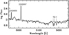 |
Fig. A.1. Stacked spectrum of the centre of the NGC 5474 bulge, smoothed with a 5 px boxcar filter. The most prominent emission and absorption lines are labelled. The flux scale is in arbitrary units. |
Unfortunately we found out, a posteriori, that significant residual velocity shifts (up to ∼30 km s−1) were present between the various science spectra and in the measures of the velocity difference from emission and absorption lines. Therefore, we conclude that the quality of the observational material and, in particular, the reliability of the wavelength calibration were not sufficient to reach our scientific goal, which was challenging given the observational set-up.
All Tables
All Figures
|
Fig. 1. RGB colour image of NGC 5474 obtained with SDSS images in g, r, and i band, for the blue, green, and red channels, respectively. North is up and east is to the left. The white circle is centred on the centre of the bulge. |
| In the text | |
|
Fig. 2. Images of NGC 5474 at different wavelengths. Left: GALEX-FUV, centre: SDSS-i, Right: continuum-subtracted Hα image (retrieved from NED, where it is attributed to Dale et al. 2009). All the images have the same scale and are aligned. The small red circle is the photometric centre of the bulge, the wide red circle has radius = 30.0″ and encloses the bulge, the small cyan square is the kinematic centre of the H I disc (according to Rownd et al. 1994), and the wide blue circle is centred on this point and has a radius = 240.0″. North is up and east is to the left. |
| In the text | |
|
Fig. 3. Surface brightness profile of the bulge of NGC 5474 in the SDSS i band. The continuous line is the Sérsic model that best-fits the observed profile. |
| In the text | |
|
Fig. 4. Upper panel: HST ACS F814W zoomed image of the central part of the bulge with intensity cuts chosen to make the stellar nucleus visible. The concentric circles provide the scale of the image and help the eye to appreciate that the nucleus resides at the centre of the bulge. Lower panel: surface brightness profile of the stellar nucleus in both the ACS bands. The continuous line displays the King (1966) model that fits the observed profiles. The parameters of the model are reported in the panels. The deviation from a smooth profile observed around log(R) = 0.75 is due to a relatively bright source projected onto the outskirts of the nucleus. |
| In the text | |
|
Fig. 5. HST ACS drizzled image of NGC 5474 in the F814W filter. The intensity contours are at 0.04, 0.08, 0.12, 0.25, 0.5, 1.0, and 2.0 e− s−1. The black circle marks the position of the kinematic centre of the H I disc. |
| In the text | |
|
Fig. 6. Upper panel: CMD from the HST catalogue. Lower panel: CMD illustrating the boxes adopted to select the various populations. |
| In the text | |
|
Fig. 7. CMD in different radial annuli, from the centre of the bulge to the edge of the ACS image. For R ≳ 50.0″ we split the annuli in their northern and southern halves (NH and SH, respectively) in order to highlight the asymmetry in the surface density related to the SW over-density. In the corresponding panels, we also report the ratio between AGB and RGB stars. The horizontal grey line marks the position of the RGB tip as determined from the whole sample. This series of CMDs also clearly illustrate the severe effect of the increasing incompleteness towards the centre of the most crowded substructure, i.e. the bulge, with the limiting magnitude dropping by nearly 2 mag from R > 30.0″ to R < 10.0″. |
| In the text | |
|
Fig. 8. Density map of the YOUNG sample obtained with TOPCAT. The axis are RA and Dec (in degrees) in sin projection. North is up and east is to the left. The colour is proportional to the square root of the local density; darker tones of blue traces higher density levels. The two asterisk symbols superimposed on the map mark the position of the centre of the bulge and of the dynamical centre of the H I disc (from Rownd et al. 1994), from north to south, respectively. |
| In the text | |
|
Fig. 9. Same as Fig. 8, but for the AGB sample. Here the colour code goes from warm colours (low density) to cold colours (high density). |
| In the text | |
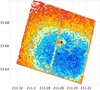 |
Fig. 10. Same as Fig. 9, but for the RGB sample. |
| In the text | |
|
Fig. 11. Stars of the YOUNG sample (in blue) are superposed to stars of the RGB sample (in grey) in a map with the same arrangement and symbols as in Fig. 10. |
| In the text | |
|
Fig. A.1. Stacked spectrum of the centre of the NGC 5474 bulge, smoothed with a 5 px boxcar filter. The most prominent emission and absorption lines are labelled. The flux scale is in arbitrary units. |
| In the text | |
Current usage metrics show cumulative count of Article Views (full-text article views including HTML views, PDF and ePub downloads, according to the available data) and Abstracts Views on Vision4Press platform.
Data correspond to usage on the plateform after 2015. The current usage metrics is available 48-96 hours after online publication and is updated daily on week days.
Initial download of the metrics may take a while.