| Issue |
A&A
Volume 633, January 2020
|
|
|---|---|---|
| Article Number | A158 | |
| Number of page(s) | 16 | |
| Section | The Sun | |
| DOI | https://doi.org/10.1051/0004-6361/201937051 | |
| Published online | 24 January 2020 | |
Coronal energy release by MHD avalanches: Heating mechanisms
1
School of Mathematics and Statistics, University of St Andrews, St Andrews, Fife KY16 9SS, UK
e-mail: This email address is being protected from spambots. You need JavaScript enabled to view it.
; This email address is being protected from spambots. You need JavaScript enabled to view it.
2
Space and Atmospheric Physics, The Blackett Laboratory, Imperial College, London, SW7 2BW, UK
3
Centre for Fusion, Space and Astrophysics, Department of Physics, University of Warwick, Coventry, CV4 7AL, UK
Received:
4
November
2019
Accepted:
14
December
2019
Abstract
The plasma heating associated with an avalanche involving three twisted magnetic threads within a coronal loop is investigated using three-dimensional magnetohydrodynamic simulations. The avalanche is triggered by the kink instability of one thread, with the others being engulfed as a consequence. The heating as a function of both time and location along the strands is evaluated. It is shown to be bursty at all times but to have no preferred spatial location. While there appears to be a level of “background” heating, this is shown to be comprised of individual, small heating events. A comparison between viscous and resistive (Ohmic) heating demonstrates that the strongest heating events are largely associated with the Ohmic heating that arises when the current exceeds a critical value. Viscous heating is largely (but not entirely) associated with smaller events. Ohmic heating dominates viscous heating only at the time of the initial kink instability. It is also demonstrated that a variety of viscous models lead to similar heating rates, suggesting that the system adjusts to dissipate the same amount of energy.
Key words: Sun: corona / Sun: magnetic fields / magnetohydrodynamics (MHD) / methods: numerical
© ESO 2020
1. Introduction
Attempts to explain the release of large amounts of energy in the magnetically confined solar atmosphere have frequently attributed it to magnetic reconnection in many newly forming current sheets (reviewed, for example, by Klimchuk 2006; Parnell & De Moortel 2012). Over the years, a number of processes have received considerable attention, and this paper focuses on two of these. The kink-mode instability is initiated by footpoint motions that twist a coronal flux tube to a degree such that the condition for marginal stability is exceeded. Extensive studies of the conditions for the onset of instability have been carried out (e.g. Hood & Priest 1979; Velli et al. 1990; Browning & Van der Linden 2003) within the framework of linearized magnetohydrodynamics (MHD). The twist of the flux tube has been defined to be Φ = (2L/a)Bϕ/Bz, where Bϕ is the azimuthal field, a is the flux tube radius, and the z axis connects the two parallel photospheric planes, where the footpoints of the flux tube are anchored and which are separated by a distance of 2L; typical critical twists are of the order of 3π–6π, depending on the equilibrium used. Simulations of the non-linear phase of the instability show that fast reconnection arises (e.g. Browning & Van der Linden 2003; Hood et al. 2009, 2016), yielding a very fragmented current structure.
Other work has addressed coronal energy release through the concept of an MHD “avalanche”. Originating with the work of Lu & Hamilton (1991), a stressed coronal magnetic field reaches a state where a local instability, or lack of equilibrium, leads to the spreading of energy release over a large volume (defined as an “event”). The generality of the idea is discussed by Vlahos & Isliker (2016). However, such avalanche models rely, in general, on a set of “rules” that determine when energy release can arise, and so determine the spatial extent of the process (temporally, the entire event occurs in one time step). We are not aware of any demonstrations of correspondence of these rules to the MHD equations. In particular, the processes invoked in these models have not, to date, been demonstrated fully from the MHD equations, although computational limitations can be held largely responsible.
In a series of recent papers, we have begun to combine these two approaches by considering “avalanches” in three-dimensional MHD simulations, and, in particular, the role of the kink instability in triggering an MHD avalanche. We have demonstrated that a single kink-unstable constituent thread within a coronal loop can destabilize a neighbouring, stable one (Tam et al. 2015), and that a single unstable thread in an array of twenty-three can lead to the destabilization of many of the others (Hood et al. 2016). In this earlier work, the loops were not driven by photospheric motions beyond instability. More recently, Reid et al. (2018, hereafter, Paper I) look at a driven system of three neighbouring strands, which are continually driven at the photosphere. One becomes unstable, engulfing the other two, and the continual driving leads to a braided system that undergoes continual dissipation.
In many multi-dimensional MHD models, such as the one described in Paper I (and references therein), the coronal energy release is intermittent, occurring in discrete bursts when summed over the simulated volume. However, how and where such “burstiness” heats the plasma has not been investigated in depth. For example, we inquire about the spatial and temporal heating along a field line (or flux element). Such information is essential for determining the subsequent field-aligned evolution of the heated plasma. This paper has two main objectives. One is to present such heating functions in the context of the three-thread avalanche model introduced in Paper I. The second is to discuss the relative roles of viscous and Ohmic heating in this model, and, in particular, where and when they contribute to the total heating.
Section 2 presents the equations solved and details of the model. Section 3 recapitulates briefly the outcome of Paper I and examines how the global (i.e. spatially integrated) heating and its Ohmic and viscous components depend on the numerical resolution of the simulation. Section 4 demonstrates the temporal and spatial dependence of the heating along a selection of field lines in different parts of the computational domain, as well as the relative importance of the two dissipative processes. Finally, in a series of Appendices, we provide extensive information about the viscous and resistive models used in the Lare3d code.
2. Basic model
The avalanche model has been summarized in the Introduction and is described fully in Paper I; a brief summary suffices here. As represented in Fig. 1, the model comprises three twisted magnetic threads (also known as strands) with footpoints fixed to the photosphere, undergoing twisting from continual rotational motions being applied there. These threads are considered to be a substructure within a larger coronal loop, modelled as the rest of the domain outside the driven threads.
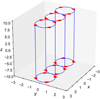 |
Fig. 1. From Paper I, the geometry of the three-thread model and associated driving motions on the boundary, indicated by the direction of the arrows at z = ±10. Each thread has a dimensionless diameter 2a, where a = 1.0. |
In their dimensionless form, the MHD equations are solved with the Lare3d code of Arber et al. (2001), neglecting thermal conduction, optically thin radiation, and gravity:
 (1)
(1)
 (2)
(2)
 (3)
(3)
 (4)
(4)
where  , ρ is the mass density, v the plasma velocity, B the magnetic field, P the gas pressure, η the resistivity, ε = P/ρ(γ−1) the specific internal energy (where γ = 5/3 is the ratio of specific heats), and j = ∇ × B the current density. Typical values for length, mass density, and magnetic field, L0 = 1 × 10⁶ m, ρ0 = 1.67 × 10⁻¹² kg m−3, and B0 = 2 × 10⁻³T = 20 G, respectively, have been used in these normalized forms. These provide a reference Alfvén speed
  (μ0 = 4π × 10−7 H m−1 is the familiar permeability of a vacuum, removed from the equations by the normalization), Alfvén travel time across L0
 , magnetic energy density W0 = 3.18 J m−3, and current density j0 = 1.59 × 10⁻³ A. In Table 1, these we compare with values typical of the strong fields in active regions and of weak fields in the quiet Sun.
Typical and normalizing values.
There are two viscosities imposed in Lare3d: in Eq. (2), there is a force per unit volume from the shock viscosity, Fshock, and one from a “background”, uniform viscosity, Fvisc.. Associated with these are heating terms in the energy equation, respectively Qshock and Qvisc.. The first of these is designed to treat shocks such that the Rankine-Hugoniot relations are satisfied, while the second is useful for damping disturbances that propagate in the domain in response to the initial evolution. Both are fully discussed in the Appendices. Appendix A.1 presents a simple outline of the shock viscosity model used, Appendix A.2 outlines the forms of Fvisc. and Qvisc., and Appendix B demonstrates that the total viscous heating to be approximately independent of the details of the viscosity models and the level of the background viscosity. The kinematic viscosities are normalized with respect to vAL0 and the default dimensionless coefficient in the background viscosity, used except where otherwise stated, is μ = ρν = 10−3; sensitivity to this choice is discussed in Appendix A.2.
In Eqs. (3) and (4), the resistivity has the form:
 (5)
(5)
where ηb is a background level of resistivity, here set to zero, and η0 an anomalous resistivity, included where the magnitude of current density exceeds a critical value, jcrit.. Apart from some parameter studies in Appendix C, our base case has a dimensionless anomalous resistivity of η0 = 0.001, imposed only where current exceeds jcrit. = 5.0. This critical level of current, similar to previous work (Tam et al. 2015; Hood et al. 2016), allows the undamped growth of the current prior to instability, and is triggered by the formation of a current sheet during the initial instability. The resistive coefficient η is normalized with respect to μ0vAL0 (= 1.73 × 10⁶ Ω m). Further remarks on the plasma resistivity model can be found in Appendix C. It should also be noted that viscous and resistive models differ among three-dimensional MHD codes; this is addressed further in the discussion.
The computational domain has dimensionless lengths −3 ≤ x, y ≤ 3, −10 ≤ z ≤ 10, with the z-coordinate being along the axis of the untwisted central loop and each twisted thread having a radius of L0 (see Fig. 1). This was modelled using three separate grids of 1282 × 512, 2562 × 1024, and 5122 × 2048 cells in the x, y, and z directions. Variation of the resolution is considered in some of the simulations described below; but, unless otherwise stated, the results use the highest resolution. The boundary conditions impose periodicity in x and y; in z, they hold zero normal derivative on all variables other than the velocity.
The initial conditions comprise a uniform plasma with a magnetic field in the z-direction, along the threads. At both footpoints of the threads, rotational motions in the x, y-plane were centred at (x,y) = (0,0) for the first thread, (2,0) for the second, and (−2,0) for the third, such that the three threads touch each other along y = 0. Defining a local radial coordinate r for each thread, the rotational velocity is:
 (6)
(6)
and is imposed throughout the simulation. The maximum speeds are chosen to be 0.05, 0.02, and 0.02, respectively (achieved with v0 = 0.21, 0.084, 0.084) and the dimensional radii take on the value a = 1.0. These values ensure that the driving is both significantly sub-Alfvénic and faster than any resistive footpoint slippage of the field lines (e.g. Bowness et al. 2013).
3. Global energetics
3.1. Overall behaviour
The overall behaviour of the three-strand avalanche was described fully in Paper I; the results can be summarized by a plot of the instantaneous heating as a function of time, shown by the blue curve in Fig. 2. The initial photospheric motions take the strands through a sequence of equilibria, with the magnetic energy growing quadratically in time. Alfvén waves generated at the start of the driving are damped by the background viscosity (see Figs. 3 and 4 of Paper I). Marginal stability of the central thread is passed at t ≈ 100, leading to the onset of the kink instability. This is identified by an exponential growth in the kinetic energy (Fig. 11 of Paper I), by the formation of a strong, crescent-shaped current sheet in the mid-plane (Fig. 5 therein), and by a gradual rise in the heating (Fig. 2). Fast reconnection facilitated by the anomalous resistivity leads to the initial release of magnetic energy; the first large spike in the total heating occurs at t = 200, indicated by the first vertical dashed line. The unstable, rapidly evolving central thread engulfs the outer two in turn, as a mini-avalanche, accompanied by major energy releases at t = 250 and t = 350. Thereafter, the continually driven system continues to produce releases of small bursts of energy, again indicated by the dashed vertical lines in Fig. 2. These bursts are superposed on a fairly steady level of total heating, suggestive of a “background” heating prevailing in the volume as a whole. We return to the nature of this background in Sect. 4.1.
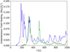 |
Fig. 2. Instantaneous total heating as a function of time, from the photospheric velocities given by Eq. (6) (blue). The red dotted vertical lines mark large heating events, as identified in Figs. 9–11 of Paper I. The green curve indicates the total heating in a similar simulation, with the rotational velocity of each thread halved. |
In order to understand the effect of resolution on the results, the same numerical experiment was performed using the three grids mentioned in Sect. 2, with the same values for the diffusion coefficients in all cases. In Fig. 3a, the evolution over time of the volume-integrated magnetic energy is shown in the upper panels. (The dimensionless magnetic energy at t = 0 is  , almost all of which is associated with the regions outside the threads, and so, for clarity, the difference from this is shown in the upper left panel.) It is clear, firstly, that the initial instability and subsequent engulfing of the two outer threads before t = 400 are largely independent of the chosen grid, and, secondly, that while the details after this time differ from case to case, roughly the same level of dissipation arises. We remark that a steady state is not reached after t = 1000 (see Paper I) and that this holds for all resolutions. (Further integration is restricted by the available computational resources.) Figures 3b,c, and d show the kinetic energy, instantaneous heating, and viscous heating, respectively, as functions of time. The kinetic energy is small in all cases, but, unlike the change in magnetic energy, shows temporal structuring that differs between the various grids, even as soon as the onset of the initial kink mode. This behaviour is also seen in the total and viscous heating rates, although, for these, the agreement is better in the initial kinking. This indicates that, despite the overall rate of dissipation in the system being similar for all models, the details of how this happens, in other words the properties of the localized regions of viscous and Ohmic heating, do depend on the resolution.
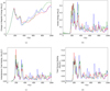 |
Fig. 3. Evolution of magnetic energy (panel a), kinetic energy (panel b), instantaneous total heating (panel c), and total viscous heating (panel d) in the domain. Results are shown for resolutions 1282 × 512 (blue), 2562 × 512 (red), and 5122 × 2048 (green). Magnetic energy is shown as a change from its initial, potential level. We remark that total and viscous heating are on different vertical scales. |
Considering these results physically is dependent upon the prescribed normalizing scales. The dimensionless figures presented can be read with any normalizing values, but, for example, with those in Table 1 for an active region, the change in magnetic energy peaks at 1.7 × 10²² J, the kinetic energy at 8.6 × 10²⁰ J, and the heating at 4.4 × 10²⁰ J s−1.
3.2. Relative importance of shock, viscous, and Ohmic heating
In real plasmas, viscous and Ohmic dissipation can lead to heating of ions and electrons, respectively. Further, the field-aligned electric field associated with resistivity can lead to acceleration of particles. While, for high densities and low temperatures, equilibration between the species can occur rapidly, this may not be the case in certain coronal parameter regimes (Braginskii 1965; Bradshaw & Cargill 2013; Barnes et al. 2016a,b), so it is of interest to investigate the relative roles of the two dissipative processes.
The left panel of Fig. 4a shows separate viscous and Ohmic heating rates and the right panel the ratio of viscous to Ohmic heating for three different resolutions as a function of time, with the same dimensionless coefficients of diffusion in each. The components of the heating rise and fall approximately (although not exactly) in phase. One might expect a small lag of viscous heating with respect to Ohmic owing to the need for reconnection to occur before shocks can form (for example, the formation of the first helical current sheet must precede the formation of slow shocks, as discussed in Bareford & Hood 2015), and this is evident at t = 200. However, at later times, such information is likely to be lost in the integration of heating rates over the entire simulation volume.
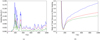 |
Fig. 4. Panel a: instantaneous total heating (blue), divided into that from Ohmic dissipation (green) and viscosity (red; the sum of shock and background viscosities). Panel b: ratio of total viscous to Ohmic heating, for simulations with resolutions 1282 × 512 (blue), 2562 × 512 (red), and 5122 × 2048 (green). |
The right panel indicates that, at the time of the first instability, Ohmic heating is more important, but, thereafter, we find a predominance of viscous heating, in common with some MHD simulations (e.g. Bareford & Hood 2015), but not others (e.g. Rappazzo et al. 2008). However, in Fig. 4b, the ratio of viscous to Ohmic heating is shown as a function of resolution, with less well resolved simulations having a predominance of viscous heating. With increasing resolution, shock heating decreases and converges to its appropriate, physically motivated level.
3.3. Mass motions associated with the avalanche
Another important diagnostic of the energy release is the associated mass motions. While the kinetic energy is relatively small (see Sect. 3.1), it is of interest to see how the flows break down into components parallel and perpendicular to the magnetic field. The total kinetic energy and its components are shown in Fig. 5 for the highest resolution simulation. The dominant kinetic energy lies in the perpendicular component, although after the initial instability there is a significant field-aligned component, indicative of there being strong localized pressure enhancements associated with the reconnection; the consequence of these field-aligned flows is discussed later. The major flows are associated with the initial kinking and engulfment of the outermost of the three strands.
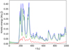 |
Fig. 5. Evolution over time of total (blue), parallel (red), and perpendicular (green) volume-integrated kinetic energy. |
3.4. Reduced photospheric velocities
Models of the corona often require footpoint velocities larger than their true values, typically 1 km s−1, owing to the large coronal Alfvén speed (and consequently small time step), and to the need to avoid resistive slippage (e.g. Bowness et al. 2013). To examine the role of such velocities, we have simulated an example with all driving speeds reduced by a factor of two, and the resultant heating is shown by the green line in Fig. 2. Marginal instability is now attained at t = 200 (compared with t = 100 formerly), and the subsequent energy release peaks at t = 325, compared with t = 185, while the second peak arises at t = 505, compared with t = 335. Thus, while the overall disruption of the threads is delayed by the slower driving, the delay is not a precise factor of two following marginal instability. In fact, the delays between the first and second maxima are 180 and 150 Alfvén times. This implies that the evolution following the first instability is, at least partially, dependent not only on the boundary motions themselves, but on internal dynamics within the threads. In particular, there is now a decoupling between the slower onset of the kink instability in the outer threads and their being engulfed by the central one. After the second peak, we again find a bursty energy release following from each, although the slower driving speed gives a superficially smoother heating, as seen in these integrated quantities.
4. Local behaviour
In order fully to evaluate the coronal response to the heating, it is necessary to examine how heating is distributed along individual field lines. This is because the response to coronal heating is largely through the field-aligned hydrodynamic response, which has been the subject of numerous studies using one-dimensional hydrodynamics with arbitrary heating functions. Obtaining the correct response to heating is more difficult in three-dimensional models on account of the need for a very fine grid in the steep transition region and consequently for a small time step. Indeed, Bradshaw & Cargill (2013) demonstrated that lack of sufficient resolution in the transition region leads to incorrect coronal densities. The heating functions obtained here could be used as realistic (less arbitrary) input in such hydrodynamic models and this will be addressed in future work.
4.1. Heating on individual field lines
We select six field lines as being representative of different parts of the computational domain. All are tracked from a point on the bottom photospheric plane (z = −10), their position there being determined by advection with the form given by Eq. (6), such that these field lines are, theoretically, the same ones throughout the duration of the simulation. Three field lines begin in the central thread, one on the axis (i.e. with twist but no driving), one near the radius of maximum driving, and the third beyond that radius. The other three begin in each of the other two driven threads, and in the region that is not being driven. These starting points are shown in Fig. 6, and the field lines are subsequently referred to as (a)–(f). Trajectories of field lines are integrated using a fourth/fifth-order Runge-Kutta-Fehlberg scheme. Local plasma properties define heating in each of the cells across the three-dimensional grid. From these, local viscous and Ohmic heating contributions are inferred at each of the discrete, finite segments tracing the field line path. The results are shown in Figs. 7–11.
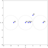 |
Fig. 6. Distribution, at t = 0 and on z = −10, of the six field lines that are tracked from the lower boundary, along which the heating is calculated in subsequent figures. The dotted circles represent the initial location of the three threads, and the domain in which they are driven. |
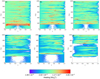 |
Fig. 7. Contours of heating as a function of time along the six field lines shown in Fig. 6. Field lines (a)–(c) are in the upper row, and (d)–(f) in the lower. The horizontal axis shows distance along the field line, normalized to the interval [0.0,1.0], the vertical axis shows time, and the contours are scaled logarithmically across four orders of magnitude. The location on the boundary from which each field line is traced is advected in time by the driving velocity, such that the same field line is theoretically tracked over time. |
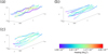 |
Fig. 8. Field lines traced and plotted in three dimensions, with shading according to the total heating experienced along them, at (a) t = 200, (b) t = 400, and (c) t = 700. The colouring is logarithmically scaled with the heating. |
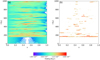 |
Fig. 9. For field line (b) (shown in Fig. 7b), the viscous (panel a) and Ohmic (panel b) constituents of heating, plotted in contours generated in like manner. Again, the colour scale is logarithmic. |
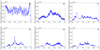 |
Fig. 10. Total heating along the field lines in Fig. 7, averaged in time. The results here are shown on a linear scale. |
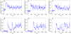 |
Fig. 11. Total heating on the field lines in Fig. 7, integrated along the field lines and then averaged over their lengths. The results here are shown on a logarithmic scale. |
Figure 7 shows the heating along these field lines, plotted as contours in space (horizontal axis) and time (vertical axis). The intensity of the heating is indicated in the colour bar. In this figure, distances along each field line are normalized by the total length of each field line, since the length can change in time as the footpoints are rotated and reconnection occurs. We have confirmed that this is a relatively small change; the maximum extension over the dimensionless length of 20 is a few percent at the time of marginal stability of the initial kink mode. The full spatial distribution of the heating experienced by a sample of field lines at a single instant in time is more readily illustrated in Fig. 8. Here, a number of field lines are traced, at t = 200, t = 400, and t = 700, and shaded by their total heating. At each of these times, we trace the same field lines, based on their motion on the lower boundary plane. In addition to field lines (a)–(e) discussed above, additional ones are selected, in order to provide a broader coverage of the simulated volume.
While field lines (a)–(e) show weak initial heating owing to the viscous damping of Alfvén waves generated by the photospheric motions, the commencement of significant heating is clear in each panel from the location of abrupt change in colour and arises at t = 150 for field line (a), at t = 180 for (b), at t = 190 for (c), at t = 220 for field line (d), and at t = 310 for field line (e). We discuss field line (f) shortly. In general, after the initial instability, the magnitude of the heating events along of all of the field lines varies quite significantly, but there is no obvious preferred spatial location for heating, other than in the central 90% of the loop, although the absence of plasma stratification may play a role in this. There are, on the other hand, significant differences between the six field lines. At the time of the peak instability, the heating is strong along almost the entire length of field line (a), largely from Ohmic heating. After this, there are some strong, localized heating peaks on this field line, triggered by smaller reconnection events far away from the footpoints. At a slightly later time, field lines (b) and (c) undergo marginally weaker heating, followed by smaller bursts.
Figure 7d and e demonstrate that, once they are disrupted, the heating in the other driven threads behaves in a similar manner, namely an extended initial burst and then localized small bursts. The major early events are consequent to each thread merging with the central one; thereafter, the reconnection is largely indiscriminate and evenly distributed across the growing region of non-potential field. However, the level of heating is weaker along these field lines compared with those within the central thread, as may be expected given their slower driving. At later times, after t = 600, stronger heating commences once these two threads are engulfed in the avalanche, this being earlier in the second thread than in the third. Thereafter, the heating profile is similar, but generally of lesser intensity.
The heating of field line (f), which starts within the outer potential region, is of considerable interest. Despite undergoing no driving, Fig. 7f demonstrates how a field line traced from the initially potential field, can be heated once it has reconnected with field lines of the driven threads. Because this field line is in the potential region just outside the central thread, it is rapidly engulfed as that thread becomes unstable. However, the subsequent spatial and temporal distribution of heating looks very similar to Fig. 7d and e.
Figure 9 shows the contours of viscous (a) and Ohmic (b), using the same colour scale, for field line (b). The Ohmic heating is very localized, as it occurs only in regions where the critical current is exceeded. The viscous heating has regions of strong heating that are closely correlated with the strong Ohmic heating.
The six panels of Fig. 10 show the time-averaged heating as a function of distance along the field lines (i.e. by averaging vertically in Fig. 7). As mentioned earlier, there is no evidence that heating is concentrated in one specific location along the axis of the central thread, rather there are heating bursts localized over small spatial intervals. However, the other threads do show localized spikes and these can largely be attributed to single events. For example, for field line (b), the peak in the middle is because of disruption of the second thread by the kink-unstable central thread and a subsequent strong heating event at t = 700. Field line (e), from the third thread, has two smaller, broader peaks around s = 0.3 and s = 0.8 that are both caused by heating associated with the disruption of this thread during the avalanche. Field line (f), initially in the potential region, has a more rounded heating profile, with little heating at the footpoints and, except one spike at s = 0.3, the maximum heating near the middle of the field line. However, it should be noted that the limited time for which the simulations were performed emphasizes these spikes over a broad level of dissipation in the resultant turbulent medium. A feature of all these plots is that there appears to be a fairly steady level of heating exceeding  in 10a, falling to
  in 10f, but, in fact, this is a consequence of the temporal average in Fig. 10.
Figure 11 shows the spatially averaged heating along the six field lines as a function of time, demonstrating a number of characteristic features. There are strong bursts of heating initially in all cases, as the instabilities and initial avalanche stages proceed. However, in the three lower panels, these are more evident when compared with the background level. This suggests the fact that, in the strongly driven region, there is a state after t ≈ 300 in which little build-up of magnetic energy is permitted and the heating rate varies by a factor somewhat larger than 10. In the outer regions, the strong bursts are more discrete, suggesting energy build-up is feasible. The magnitude of the events now varies by a factor of 100.
The second interesting feature of these results concerns what we have previously referred to as the background. In all panels of Fig. 11, while there is a clear minimum in the heating rate, that minimum is only attained at a few times. Instead, there is a range of heating rates. This suggests that any low-level “numerical” heating is almost always superseded by some ubiquitous “physical” heating, understood to mean that the imposed viscous and resistive diffusion are operative. Further, the background that we noted in Fig. 2 is, in fact, a superposition of an evenly dispersed viscous action and several small, discrete, and far more impulsive events.
4.2. Spatial location of heating and distribution
The distribution of the instantaneous total, viscous, and Ohmic heating in the mid-plane, z = 0, is illustrated in Fig. 12 at t = 200, t = 400, and t = 700. An intense current is among the characteristic hallmarks of a kink instability. Figure 13 shows the current in the mid-plane at t = 200, t = 400, and t = 700, respectively. Fragmentation and proliferation in the current layers develops over time, with the solid, pronounced current as the instability emerges being replaced with a network of small, complex structures enabling dissipation, magnetic reconnection, and small heating events.
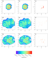 |
Fig. 12. Contours in the mid-plane of total heating (left column), viscous heating (middle column), and Ohmic heating (right column), at t = 200 (top row), t = 400 (middle row), and t = 700 (bottom row). The total heating in the plane in each plot (in dimensions |

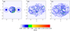 |
Fig. 13. Contours of the magnitude of total current (|j|) in the mid-plane (z = 0) at t = 200 (panel a), t = 400 (panel b), and t = 700 (panel c). The colour bar changes around the critical threshold for anomalous resistivity, jcrit. = 5.0, and shows current slightly below this threshold in green. |
We note that the strongest heating is four orders of magnitude larger than the weakest. We have used a minimum heating threshold of 10−6 and neglected any cells with a lower value.
At t = 200, the strongest heating locations (orange and red regions) are coincident with the regions of Ohmic heating. This is not surprising, since the Ohmic heating, on account of its anomalous nature, is far more localized, but, where it does occur, its magnitudes are greater and have a minimum value ( ), corresponding to the jcrit. for the onset of resistivity. In addition, the kink instability, which initiates the avalanche process, forms a strong helical current sheet, forming the crescent of Ohmic heating seen strongly in Fig. 12c. The strongest viscous heating sites are closely associated with the Ohmic heating sites and there is evidence of heating in the slow-mode shocks in the reconnection outflow regions (discussed by Bareford & Hood 2015). The weaker heating is more distributed throughout the unstable magnetic thread and is wholly from the viscous contribution. This heating is almost certainly dependent upon the form of the viscosity used and upon the size of the coefficients in the shock viscosity.
At t = 400, the Ohmic heating occurs in a large number of small regions of strong current, and the strongest regions of viscous heating coincide with the strongest Ohmic heating sites. However, there are many fine, wisp-like structures in the intermediate values of viscous heating (≈10−3). The weakest viscous heating (< 10−5) now covers the majority of the remainder of the computational domain. Thus, there is always some weak, entirely viscous, heating. When integrated over the plasma volume, this corresponds to the weak background heating seen in Fig. 3c.
In order to determine whether the more numerous, weak features in the heating contribute more to the total than the less common but larger, we calculate heating frequency histograms. In Fig. 14, the histograms show the distributions of the viscous and Ohmic constituents of the total heating, as functions of heating density. We remark that these histograms count only the specific, local heating felt at each computational cell, which may not necessarily correspond to an “event”, as these may be spread across several adjacent cells and many time steps; to isolate such events discretely involves an analysis well beyond the scope of the present paper (but see, for example, Guerreiro et al. 2015; Kanella & Gudiksen 2017). There is a fairly clear distinction between Ohmic and viscous heating, the former dominating at high energies and cutting off abruptly at  . In part, this is a consequence of the use of a critical current to turn on resistivity; but it should also be noted that there are comparatively few viscous events at such energies, with the viscous heating predominating at lower energy. In Fig. 14a, there is some evidence of a three-part power law at t = 200, as indicated by the dashed line segments. However, there is no evidence of a power law at the later times shown.
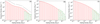 |
Fig. 14. Histograms of the constituents of total heating, viscous (red) and Ohmic (green), in each cell in the domain, at times t = 200 (panel a), following the instability of the central thread, t = 400 (panel b), following the subsequent evolution of the instability across the domain, and t = 700 (panel c), much later. The histograms are produced logarithmically from the values of heating found at each cell within the computational domain. |
5. Conclusions and discussion
In this paper, we have developed the avalanche model of three threads first discussed by Paper I, in order to study the plasma heating arising from the energy dissipation. Globally, heating is shown first to arise as large bursts associated with an initial kink instability in one thread, but thereafter to evolve to a series of smaller heating events. These macroscopic results seem to be largely robust to a range of chosen viscosity and resistivity models, and to varying numerical resolution. For our chosen viscous and resistive models, resistive heating is the more important at the time of initial kink instability, but viscous heating subsequently becomes the more important. Resistive heating also occurs as a relatively small number of large “events”, whereas viscous is generally associated with smaller events.
We have also determined the specific time-dependent heating functions along a number of field lines. These show no obvious spatial preference, bursts of energy being released along approximately 90% of field lines, although after the initial kinking, these are localized. Temporally, local heating remains highly intermittent and impulsive, indeed arguably more so than in the volume-integrated results. This field-aligned heating can be considered as input for one-dimensional models of loop plasma evolution, and this will be returned to in a future paper.
In Paper I and here, we have used viscous and resistive coefficients that are intended to describe, in particular, the physics of shocks and the onset of magnetic reconnection in regions with strong currents. These transport coefficients are, of course, large in comparison with those produced by the parameter values from classical theory (e.g. Braginskii 1965), but this artificial scaling is essential, given the inability of current MHD codes to simulate such plasma transport in a realistic way. We showed that our coefficients operate in such a way as ensures that the build-up of energy and subsequent dissipation occur.
However, our prescription is not unique, and other workers have adopted alternative approaches. The simplest approach is used, for example, in reduced MHD and involves an assumption of incompressibility, so eliminating the presence of shocks and field-aligned flows. Instead, simple viscous and resistive coefficients are used, the two usually set equal, and expressible as a hyper-diffusion, partly in an attempt to localize diffusion at regions of intense current and/or vorticity, and partly to enable the implementation of an efficient spectral method. (A similarly simple, abrupt, piecewise form, as used here and frequently also by others, is not readily amenable to such a spectral approach.) In view of the importance of slow-mode shocks, found by ourselves (on which we have for want of space been unable to expand here) and by others, RMHD risks missing important aspects of coronal energy dissipation.
Our chosen switch for the initiation of resistivity is, admittedly, arbitrary and other models may lead to different results. Such models are based on the notion that an anomalously high resistivity can be triggered when the electron drift associated with the current exceeds some critical value, often a given fraction of the ion thermal speed. For example, Bareford & Hood (2015) use a critical current dependent on plasma parameters, especially including a linear proportionality to temperature through thermal velocity and Larmor radius. Consequently, as soon as any heating arises, the critical current increases rapidly and so precludes further Ohmic heating, although there are cases where the temperature increase makes a further micro-instability more likely (e.g. the supernova shock model of Cargill & Papadopoulos 1988). In contrast to our work, Bareford & Hood (2015) found very large ratios of viscous to Ohmic heating, as did a similar model of Gordovskyy et al. (2014). These models are based on the notion that an anomalously high resistivity be triggered when the electron drift associated with the current exceed a critical value, often some fraction of the ion thermal speed (so introducing the temperature dependence), and rely on simple considerations with quite a large threshold for instability. On the other hand, there are instabilities with less severe onset conditions, especially associated with lower hybrid waves. Also, resistive models can be combined, such as using a global resistive model in conjunction with a hyper-diffusion of the form often seen in RMHD, in order to dissipate in particular small currents (e.g. Gudiksen et al. 2011). Alternatively, many use codes allowing for a resistivity that scales in some way with current above a critical threshold (e.g. Pagano & De Moortel 2019; Porth et al. 2014). The topic remains to be explored in its totality, for which reason it is difficult at this stage to select any one model before all others.
While viscosity was found to be important at most times away from shocks and fine current layers, we find that our viscous model was the dominant dissipative mechanism. In reality, the fate of small-scale currents and vortices is uncertain. One possible path admits a rapid cascade to small scales at which “real” (that is, physical, without numeric or artificially high) viscosity and resistivity take over. Following Braginskii (1965), we find kinematic perpendicular viscosity  , and resistivity
  , in MKS units. Their ratio defines the magnetic Prandtl number Pm = ν/η = 9 × 10⁻²⁸nT/B2 = 13β (cf. Cargill et al. 2016), which reflects their relative balance, and which can, with coronal parameters, be less than unity, implying resistive diffusion more significant at such scales. Naturally, then, it is a subject of concern that our model finds viscous dominance and that viscous coefficients are often assumed higher (as found, for example, by Hendrix & Van Hoven 1996; Bingert & Peter 2011). Two caveats, however, apply to this. Firstly, the field-aligned viscosity, more than 108 times more effective than the transverse and with an equivalently higher magnetic Prandtl number, dissipates very efficiently the parallel flows shown in Fig. 5. Secondly, in a tangled field of the kind found after the original kink instability, it is plausible that viscous heating is enhanced by small-scale process, such as a localized Kelvin-Helmholtz instability (discussed, for example, by Browning & Priest 1984, in the context of wave heating). Nevertheless, the scaling of Ohmic heating with magnetic Reynolds number has been explored, and Ohmic heating may alone suffice for heating (Hendrix et al. 1996).
Finally, it is of interest to comment upon the link between such MHD models as presented here and such avalanche models as developed by Lu et al. (1993). The difficult in comparing the two can be seen in Fig. 14, in which we plot a distribution of “events”. These are snapshots at a given time, and are not the same as “events” in avalanche models, where the system can evolve over multiple scales until a stable state is reached. Trying to track such features in MHD models is a very difficult task (well attempted by Guerreiro et al. 2015; Kanella & Gudiksen 2017), involving a large amount of post-processing; it is unclear whether this can ultimately be achieved. In turn, this casts some shadow over some of the fundamental concepts of avalanche models, in whether the rules on which they rely are verifiable from first principles. On the other hand, it is equally true that any rules emerging from three-dimensional MHD models may be regarded with suspicion, owing to the artificial dissipative coefficients employed.
This is discussed by Arber, T. 2018. “LareXd User Guide”, University of Warwick, available at https://warwick.ac.uk/fac/sci/physics/research/cfsa/people/tda/larexd/.
Acknowledgments
JR acknowledges the support of the Carnegie Trust for the Universities of Scotland. AWH and CEP acknowledge the financial support of the STFC through the Consolidated grant, ST/S000402/1, to the University of St Andrews. AWH acknowledges support from ERC Synergy grant “The Whole Sun” (810218). TDA acknowledges the financial support of the STFC through the Consolidated grant, ST/P000320/1, to the University of Warwick. The authors are grateful to Prof. Philippa K. Browning for helpful advice and sustained discussion concerning the work. The authors are further grateful to Dr Benjamin M. Williams for the code used for all tracing of field lines for the purposes of this paper; the code uses an RKF45 scheme, details of which are presented by Williams (2018). This work used the DiRAC@Durham facility, managed by the Institute for Computational Cosmology, and the Cambridge Service for Data Driven Discovery (CSD3), part of which is operated by the University of Cambridge Research Computing, on behalf of the STFC DiRAC HPC Facility (www.dirac.ac.uk). The DiRAC@Durham equipment was funded by BEIS capital funding via STFC capital grants ST/P002293/1 and ST/R002371/1; Durham University; STFC operations grant ST/R000832/1; BIS National E-infrastructure capital grant ST/K00042X/1; STFC capital grant ST/K00087X/1; and DiRAC Operations grant ST/K003267/1. The DiRAC component of CSD3 was funded by BEIS capital funding via STFC capital grants ST/P002307/1 and ST/R002452/1 and STFC operations grant ST/R00689X/1. DiRAC is part of the National e-Infrastructure. This work used the NumPy (Oliphant 2006) and Matplotlib (Hunter 2007) Python packages.
References
- Arber, T. D., Longbottom, A. W., Gerrard, C. L., & Milne, A. M. 2001, J. Comput. Phys., 171, 151 [NASA ADS] [CrossRef] [Google Scholar]
- Bareford, M. R., & Hood, A. W. 2015, Phil. Trans. Roy. Soc. A, 373, 20140266 [NASA ADS] [CrossRef] [Google Scholar]
- Barnes, W. T., Cargill, P. J., & Bradshaw, S. J. 2016a, ApJ, 829, 31 [NASA ADS] [CrossRef] [Google Scholar]
- Barnes, W. T., Cargill, P. J., & Bradshaw, S. J. 2016b, ApJ, 833, 217 [NASA ADS] [CrossRef] [Google Scholar]
- Bingert, S., & Peter, H. 2011, A&A, 530, A112 [NASA ADS] [CrossRef] [EDP Sciences] [Google Scholar]
- Bowness, R., Hood, A. W., & Parnell, C. E. 2013, A&A, 560, A89 [NASA ADS] [CrossRef] [EDP Sciences] [Google Scholar]
- Bradshaw, S. J., & Cargill, P. J. 2013, ApJ, 770, 12 [NASA ADS] [CrossRef] [Google Scholar]
- Braginskii, S. I. 1965, Rev. Plasma Phys., 1, 205 [Google Scholar]
- Brio, M., & Wu, C. C. 1988, J. Comput. Phys., 75, 400 [NASA ADS] [CrossRef] [Google Scholar]
- Browning, P. K., & Priest, E. R. 1984, A&A, 131, 283 [NASA ADS] [Google Scholar]
- Browning, P. K., & Van der Linden, R. A. M. 2003, A&A, 400, 355 [NASA ADS] [CrossRef] [EDP Sciences] [Google Scholar]
- Caramana, E. J., Shashkov, M. J., & Whalen, P. P. 1998, J. Comput. Phys., 144, 70 [NASA ADS] [CrossRef] [Google Scholar]
- Cargill, P. J., & Papadopoulos, K. 1988, ApJ, 329, L29 [NASA ADS] [CrossRef] [Google Scholar]
- Cargill, P. J., De Moortel, I., & Kiddie, G. 2016, ApJ, 823, 31 [NASA ADS] [CrossRef] [Google Scholar]
- Gordovskyy, M., Browning, P. K., Kontar, E. P., & Bian, N. H. 2014, A&A, 561, A72 [NASA ADS] [CrossRef] [EDP Sciences] [Google Scholar]
- Gudiksen, B. V., Carlsson, M., Hansteen, V. H., et al. 2011, A&A, 531, A154 [NASA ADS] [CrossRef] [EDP Sciences] [Google Scholar]
- Guerreiro, N., Haberreiter, M., Hansteen, V., & Schmutz, W. 2015, ApJ, 813, 61 [NASA ADS] [CrossRef] [Google Scholar]
- Hendrix, D. L., & Van Hoven, G. 1996, ApJ, 467, 887 [NASA ADS] [CrossRef] [Google Scholar]
- Hendrix, D. L., van Hoven, G., Mikic, Z., & Schnack, D. D. 1996, ApJ, 470, 1192 [NASA ADS] [CrossRef] [Google Scholar]
- Hirsch, C. 2013, Numerical Computation of Internal and External Flows (Delhi: John Wiley & Sons), 2 [Google Scholar]
- Hood, A. W., & Priest, E. R. 1979, Sol. Phys., 64, 303 [NASA ADS] [CrossRef] [Google Scholar]
- Hood, A. W., Browning, P. K., & Van der Linden, R. A. M. 2009, A&A, 506, 913 [NASA ADS] [CrossRef] [EDP Sciences] [Google Scholar]
- Hood, A. W., Cargill, P. J., Browning, P. K., & Tam, K. V. 2016, ApJ, 817, 5 [NASA ADS] [CrossRef] [Google Scholar]
- Hunter, J. D. 2007, Comput. Sci. Eng., 9, 90 [NASA ADS] [CrossRef] [Google Scholar]
- Kanella, C., & Gudiksen, B. V. 2017, A&A, 603, A83 [NASA ADS] [CrossRef] [EDP Sciences] [Google Scholar]
- Klimchuk, J. A. 2006, Sol. Phys., 234, 41 [NASA ADS] [CrossRef] [Google Scholar]
- Kuropatenko, V. F. 1967, in Proceedings of the Steklov Institute of Mathematics, ed. N. N. Janenko (Providence, Rhode Island: American Mathematical Society), 74, 116 [Google Scholar]
- Lu, E. T., & Hamilton, R. J. 1991, ApJ, 380, L89 [NASA ADS] [CrossRef] [Google Scholar]
- Lu, E. T., Hamilton, R. J., McTiernan, J. M., & Bromund, K. R. 1993, ApJ, 412, 841 [NASA ADS] [CrossRef] [Google Scholar]
- Margolin, L. G. 2019, Shock Waves, 29, 27 [NASA ADS] [CrossRef] [Google Scholar]
- Oliphant, T. E. 2006, A guide to NumPy (USA: Trelgol Publishing) [Google Scholar]
- Pagano, P., & De Moortel, I. 2019, A&A, 623, A37 [NASA ADS] [CrossRef] [EDP Sciences] [Google Scholar]
- Parnell, C. E., & De Moortel, I. 2012, Phil. Trans. Roy. Soc. A, 370, 3217 [Google Scholar]
- Porth, O., Xia, C., Hendrix, T., Moschou, S. P., & Keppens, R. 2014, ApJS, 214, 4 [Google Scholar]
- Priest, E. 2014, Magnetohydrodynamics of the Sun (Cambridge: Cambridge University Press) [Google Scholar]
- Rappazzo, A. F., Velli, M., Einaudi, G., & Dahlburg, R. B. 2008, ApJ, 677, 1348 [NASA ADS] [CrossRef] [Google Scholar]
- Reid, J., Hood, A. W., Parnell, C. E., Browning, P. K., & Cargill, P. J. 2018, A&A, 615, A84 [NASA ADS] [CrossRef] [EDP Sciences] [Google Scholar]
- Spitzer, L. 1962, Physics of fully ionized gases (New York: Interscience Publishers) [Google Scholar]
- Tam, K. V., Hood, A. W., Browning, P. K., & Cargill, P. J. 2015, A&A, 580, A122 [NASA ADS] [CrossRef] [EDP Sciences] [Google Scholar]
- Velli, M., Einaudi, G., & Hood, A. W. 1990, ApJ, 350, 419 [NASA ADS] [CrossRef] [Google Scholar]
- Vlahos, L., & Isliker, H. 2016, Eur. J. Spec. Top. Phys., 225 [Google Scholar]
- Wilkins, M. L. 1980, J. Comput. Phys., 36, 281 [NASA ADS] [CrossRef] [Google Scholar]
- Williams, B. M. 2018, PhD Thesis, University of St Andrews [Google Scholar]
Appendix A: Numeric issues in Lare simulations
A.1. Shock viscosity
The Lare code implements a shock viscosity with the aim of satisfying the Rankine-Hugoniot equations at shocks1. This is required because the ideal MHD equations admit singular solutions within a finite time, which are not physically real. Small but finite viscosity would result in a continuous solution that varies rapidly over a short distance. The shock viscosities are intended to broaden regions of rapid change by providing small local dissipation, allowing the Rankine-Hugoniot relations to be satisfied. However, these shock viscosities can have other consequences, as we discuss below.
Shock viscosities use a “fictitious” pressure, here defined as p⋆. The form proposed by Kuropatenko (1967) and Wilkins (1980) for one-dimensional solutions is:
![Mathematical equation: $$ \begin{aligned} p^{\star } = \rho \left[\nu _{2}\frac{\gamma +1}{4}\left| \Delta \boldsymbol{{v}} \right| + \sqrt{\nu _{2}^{2}\left(\frac{\gamma +1}{4}\right)^{2}\left( \Delta \boldsymbol{{v}} \right)^{2}+\nu _{1}^{2}c_{\rm s}^{2}}\right]\left| \Delta \boldsymbol{v} \right|, \end{aligned} $$](/articles/aa/full_html/2020/01/aa37051-19/aa37051-19-eq18.gif) (A.1)
(A.1)
where Δv is the difference in the velocity field across a cell, ν1, ν2 are dimensionless coefficients controlling the shock viscosity, and cs is the sound speed. When ν1 = ν2 = 1.0, p⋆ is identical to the pressure difference found in the Rankine-Hugoniot relations. Considering respectively the limits cs ≫ |Δv| and cs ≪ |Δv|, ν1 and ν2 govern the linear and quadratic dependence of p⋆ on |Δv|. For specifically MHD problems, the sound speed cs is replaced with the magnetoacoustic fast-mode speed,  . In the shock tests undertaken by Arber et al. (2001), this resulted in satisfactory performance, for example in the canonical problem of Brio & Wu (1988).
The precise multi-dimensional implementation follows the approach of Caramana et al. (1998). On each edge of each cell, a force is calculated:
![Mathematical equation: $$ \begin{aligned} \boldsymbol{F^{\star }} = \rho \left[\nu _{2}\frac{\gamma +1}{4}\left| \Delta \boldsymbol{v} \right| + \sqrt{\nu _{2}^{2}\left(\frac{\gamma +1}{4}\right)^{2}\left( \Delta \boldsymbol{v} \right)^{2}+\nu _{1}^{2}c_{\rm s}^{2}}\right] \frac{\Delta \boldsymbol{{v}}\cdot \boldsymbol{S}}{\left|\Delta \boldsymbol{v}\right|} \Delta \boldsymbol{v}, \end{aligned} $$](/articles/aa/full_html/2020/01/aa37051-19/aa37051-19-eq20.gif) (A.2)
(A.2)
where ρ is evaluated on the edge, Δv the difference in velocity along the edge, and S is an area defined in the median mesh proposed by Caramana et al. (1998). This force is applied to the vertex pointed to by S, and an equal, opposing force to the other vertex on the edge. It is equivalent to the force produced by such a pressure as in Eq. (A.1) along the edge of the computational cell. Within the predictor-corrector scheme, these forces are then used in the calculation of the updated velocity, its value at each vertex being influenced by its adjacent edges. The action of these forces produces a shock heating that is applied to the internal energy. This is calculated as F⋆ ⋅ v, in the usual way.
By default, the code follows common practice in MHD in that it applies the shock viscosities everywhere, both in the presence and absence of compressions. There exists an option, further discussed here, to restrict this behaviour by using the shock viscosities only in the presence of compressions, as is more common practice in fluid dynamics and has been prescribed by literature on the subject (for example, by Wilkins 1980).
The form of pressure prescribed by Eq. (A.1) is not entirely arbitrary or unconnected with the physical equations. As noted by Margolin (2019), this forms agrees with the truncation term produced in deriving the form of the Navier-Stokes equations appropriate for a finite-volume method.
A.2. Background viscosity
A background viscosity is also applied of the form:
 (A.3)
(A.3)
 (A.4)
(A.4)
where μ = ρν is the dynamic viscosity, ν kinematic viscosity, ∇v is the gradient of the velocity vector, and we assume summation over repeated indices. Formally, this is only valid for an isothermal, unmagnetized, and incompressible plasma. In addition, the viscous coefficient μ is chosen on numerical grounds and assumed constant over the computational domain. The role of imposing this simplified, uniform viscosity is to damp MHD waves, in particular those originating prior to the instability. The effect of this viscosity and of its interaction with the shock viscosity is discussed below.
A.3. Lagrangian code: energy conservation
Lare is a Lagrangian remap code, which, at each time step, solves its governing equations on a staggered, Lagrangian grid, before remapping the results back onto the originally prescribed Eulerian mesh. The remap conserves mass and momentum, but not kinetic energy. Kinetic energy may be lost, and this effect can be particularly acute near shocks.
The code has a facility, not here used, to account for kinetic energy lost in its remapping stage. In order to remove this specific source of error in conservation of total energy, the loss may be calculated and incorporated as heating. However, any loss of magnetic energy remains a source of numerical error in the code (Arber et al. 2001).
Appendix B: Viscosity models: influence on heating
As indicated in Sect. 2, attention must be paid to how the results may be changed as the models for the viscosities are altered. Figure B.1 shows the combined and individual contributions to total heating of the shock and background viscosities, as the background (dynamic) viscosity takes on the dimensionless values 10−3, 10−4, 0.0. Figure B.2 compares, for higher resolution, the total and shock viscous heating for the previous main case (μ = 10−3), the case without background viscosity (i.e. μ = 0.0), and the case without background viscosity and limiting the role of shock viscosities to compressions.
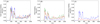 |
Fig. B.1. Contributions to instantaneous total heating, from total viscous heating (a), shock heating (b), and background viscous heating (c), comparing coefficients for background viscosity μ = ρν = 10−3 (blue), μ = ρν = 10−4 (red), and μ = ρν = 0.0 (green). |
What is clear from these comparisons is a degree of interplay between the viscosities in the code. The reduction of heating by background viscosity is not matched by a straightforward and equivalent reduction in the level of total viscous heating. Instead, the shock heating increases, this part of the formulation of viscosity not confined solely to true shocks.
To address this last point, we have restricted the application of shock viscosity to compressions (i.e. ∇ ⋅ v < 0) only, as shown in Fig. B.2, where there is clearly a lower level of shock (and therefore also total viscous) heating. However, the majority of shock heating does indeed appear to arise from compressions, suggesting that the code’s handling of shocks, although arguably too widely applied, is most active on flows that are “shocks” in the conventional, strictly compressive sense.
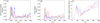 |
Fig. B.2. Contributions to instantaneous total heating from total viscous heating (a) and shock heating (b), and magnetic energy (c), for the previous μ = ρν = 10−3 level of background viscosity, as in the base case (blue); μ = ρν = 0.0 for no background viscosity (red); the same while confining the shock viscosities to act strictly at compressions only (green); and no background viscosity while applying the gradient limiters in the shock viscosity (magenta). |
Moreover, it is clear from the magnetic energy in Fig. B.2c that, after the original process of instability, a similar overall magnetic state is reached with each parameter set at t = 400. We remark that any apparent enhancement of total shock heating in the case where shock viscosities are confined to compressions is likely explained by a different preceding evolution. In such case, the heating is generally earlier, as less dissipation allows shocks to form earlier.
Expanding upon the comparison of the code’s representation of viscosity with its physical effects, it is well known (Braginskii 1965; Spitzer 1962) that the physical viscosity is dominated by the contribution from parallel velocity. Figure 5 shows that, over the course of the simulation, there is a marked shift from the entirely perpendicular velocity which is imposed at the boundaries according to the form of the driving and spreads throughout the domain, to a growing parallel velocity, which may contribute to significant (and real) viscous heating (cf. discussion).
Appendix C: Comments on resistivity models: influence on heating
In studying the kink instability, it is required that the magnetic field build up energy prior to the onset of instability. A constant “background” resistivity may lead to a slower build-up of magnetic energy. Thus, the “anomalous” resistivity should not turn on until the currents exceed the level present when the magnetic threads reach theoretical marginal instability to the ideal MHD mode; this motivated our choice of jcrit. in Sect. 2. We observe that an alternative “resistivity” model is simply to rely on numerical diffusion owing to truncation errors. While this has the merit of being important only when currents are strong, there is some evidence of a “chequerboard” instability in several of the variables (Hirsch 2013).
In realistic physical systems, classical (Spitzer 1962) resistivity is unimportant, as can be seen by frequently quoted magnetic Reynolds numbers of the order of 1012. Instead, an anomalous resistivity is likely to arise abruptly around a certain switch-on level of current: it becomes significant where a current layer forms, and length scales collapse. Whether the resistivity is owing to turbulent electric fields arising from a plasma instability or from partial electron demagnetization is unclear at this time. It should also be noted that the conditions for such physical processes to arise cannot be met in present day MHD simulations. Accordingly, we follow a common procedure and use an anomalous resistivity, with a selected threshold level well below that indicated by plasma studies.
In Sect. 3, we compare the results for different resolutions with the same value of jcrit.. Figure C.1 demonstrates the outcome of relaxing this assumption. We show three simulations, two with 5122 × 2048 points, but with jcrit. = 5.0 and jcrit. = 10.0 (blue and red curves respectively), as well as a case with 2562 × 1024 points and jcrit. = 5.0 (green curves). The former is comparable to the studies of (e.g. Gordovskyy et al. 2014; Bareford & Hood 2015), although the parametric dependence of their critical current on plasma parameters such as density and temperature is ignored. Two of these cases were run in Sect. 3, but lack of space did not permit the showing of the Ohmic heating. The three panels of Fig. C.1 show the magnetic energy, kinetic energy, and Ohmic heating. The magnetic energy shows little difference between the two higher resolution simulations, except that the reduced dissipation associated with the higher critical current enables the retention of greater magnetic energy at the onset of the instability. The higher current threshold also has smaller Ohmic heating, with the peaks lower by around a factor of two and greater kinetic energy, though the latter difference is small. Thus, despite the larger currents attainable in the high resolution model, the smaller volume associated with the finer grid leads to less heating. Comparing the two cases with jcrit. = 5.0, the principal difference is greater kinetic energy.
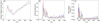 |
Fig. C.1. Comparing resistivity models, and their impact upon magnetic energy (a), kinetic energy (b), and Ohmic heating (c) across simulations with 5122 × 2048 cells and jcrit. = 5.0 (blue), 5122 × 2048 cells and jcrit. = 10.0 (red), and 2562 × 1024 cells and jcrit. = 5.0 (green). |
Finally, we investigated a smooth form of η, modelled as an hyperbolic tangent:
 (C.1)
(C.1)
which smoothly and differentiably introduced resistivity about the same threshold level, over a typical width in current density-space of δ = 0.5. This yielded qualitatively similar behaviour in overall evolution and comparable global results; the differences with the abrupt switch-on were less than induced by other factors, such as resolution.
All Tables
All Figures
|
Fig. 1. From Paper I, the geometry of the three-thread model and associated driving motions on the boundary, indicated by the direction of the arrows at z = ±10. Each thread has a dimensionless diameter 2a, where a = 1.0. |
| In the text | |
|
Fig. 2. Instantaneous total heating as a function of time, from the photospheric velocities given by Eq. (6) (blue). The red dotted vertical lines mark large heating events, as identified in Figs. 9–11 of Paper I. The green curve indicates the total heating in a similar simulation, with the rotational velocity of each thread halved. |
| In the text | |
|
Fig. 3. Evolution of magnetic energy (panel a), kinetic energy (panel b), instantaneous total heating (panel c), and total viscous heating (panel d) in the domain. Results are shown for resolutions 1282 × 512 (blue), 2562 × 512 (red), and 5122 × 2048 (green). Magnetic energy is shown as a change from its initial, potential level. We remark that total and viscous heating are on different vertical scales. |
| In the text | |
|
Fig. 4. Panel a: instantaneous total heating (blue), divided into that from Ohmic dissipation (green) and viscosity (red; the sum of shock and background viscosities). Panel b: ratio of total viscous to Ohmic heating, for simulations with resolutions 1282 × 512 (blue), 2562 × 512 (red), and 5122 × 2048 (green). |
| In the text | |
|
Fig. 5. Evolution over time of total (blue), parallel (red), and perpendicular (green) volume-integrated kinetic energy. |
| In the text | |
|
Fig. 6. Distribution, at t = 0 and on z = −10, of the six field lines that are tracked from the lower boundary, along which the heating is calculated in subsequent figures. The dotted circles represent the initial location of the three threads, and the domain in which they are driven. |
| In the text | |
|
Fig. 7. Contours of heating as a function of time along the six field lines shown in Fig. 6. Field lines (a)–(c) are in the upper row, and (d)–(f) in the lower. The horizontal axis shows distance along the field line, normalized to the interval [0.0,1.0], the vertical axis shows time, and the contours are scaled logarithmically across four orders of magnitude. The location on the boundary from which each field line is traced is advected in time by the driving velocity, such that the same field line is theoretically tracked over time. |
| In the text | |
|
Fig. 8. Field lines traced and plotted in three dimensions, with shading according to the total heating experienced along them, at (a) t = 200, (b) t = 400, and (c) t = 700. The colouring is logarithmically scaled with the heating. |
| In the text | |
|
Fig. 9. For field line (b) (shown in Fig. 7b), the viscous (panel a) and Ohmic (panel b) constituents of heating, plotted in contours generated in like manner. Again, the colour scale is logarithmic. |
| In the text | |
|
Fig. 10. Total heating along the field lines in Fig. 7, averaged in time. The results here are shown on a linear scale. |
| In the text | |
|
Fig. 11. Total heating on the field lines in Fig. 7, integrated along the field lines and then averaged over their lengths. The results here are shown on a logarithmic scale. |
| In the text | |
|
Fig. 12. Contours in the mid-plane of total heating (left column), viscous heating (middle column), and Ohmic heating (right column), at t = 200 (top row), t = 400 (middle row), and t = 700 (bottom row). The total heating in the plane in each plot (in dimensions |
| In the text | |
|
Fig. 13. Contours of the magnitude of total current (|j|) in the mid-plane (z = 0) at t = 200 (panel a), t = 400 (panel b), and t = 700 (panel c). The colour bar changes around the critical threshold for anomalous resistivity, jcrit. = 5.0, and shows current slightly below this threshold in green. |
| In the text | |
|
Fig. 14. Histograms of the constituents of total heating, viscous (red) and Ohmic (green), in each cell in the domain, at times t = 200 (panel a), following the instability of the central thread, t = 400 (panel b), following the subsequent evolution of the instability across the domain, and t = 700 (panel c), much later. The histograms are produced logarithmically from the values of heating found at each cell within the computational domain. |
| In the text | |
|
Fig. B.1. Contributions to instantaneous total heating, from total viscous heating (a), shock heating (b), and background viscous heating (c), comparing coefficients for background viscosity μ = ρν = 10−3 (blue), μ = ρν = 10−4 (red), and μ = ρν = 0.0 (green). |
| In the text | |
|
Fig. B.2. Contributions to instantaneous total heating from total viscous heating (a) and shock heating (b), and magnetic energy (c), for the previous μ = ρν = 10−3 level of background viscosity, as in the base case (blue); μ = ρν = 0.0 for no background viscosity (red); the same while confining the shock viscosities to act strictly at compressions only (green); and no background viscosity while applying the gradient limiters in the shock viscosity (magenta). |
| In the text | |
|
Fig. C.1. Comparing resistivity models, and their impact upon magnetic energy (a), kinetic energy (b), and Ohmic heating (c) across simulations with 5122 × 2048 cells and jcrit. = 5.0 (blue), 5122 × 2048 cells and jcrit. = 10.0 (red), and 2562 × 1024 cells and jcrit. = 5.0 (green). |
| In the text | |
Current usage metrics show cumulative count of Article Views (full-text article views including HTML views, PDF and ePub downloads, according to the available data) and Abstracts Views on Vision4Press platform.
Data correspond to usage on the plateform after 2015. The current usage metrics is available 48-96 hours after online publication and is updated daily on week days.
Initial download of the metrics may take a while.