| Issue |
A&A
Volume 633, January 2020
|
|
|---|---|---|
| Article Number | A12 | |
| Number of page(s) | 7 | |
| Section | The Sun | |
| DOI | https://doi.org/10.1051/0004-6361/201936453 | |
| Published online | 20 December 2019 | |
Simultaneous longitudinal and transverse oscillations in filament threads after a failed eruption⋆
1
Center of Excellence in Space Sciences India, Indian Institute of Science Education and Research Kolkata, Mohanpur 741246, West Bengal, India
2
Indian Institute of Astrophysics, Bangalore 560 034, India
e-mail: This email address is being protected from spambots. You need JavaScript enabled to view it.
3
Centre for mathematical Plasma Astrophysics, Department of Mathematics, KU Leuven, Celestijnenlaan 200B bus 2400, 3001 Leuven, Belgium
e-mail: This email address is being protected from spambots. You need JavaScript enabled to view it.
4
Instituto de Astrofísica de Canarias, 38205 La Laguna, Tenerife, Spain
5
Departamento de Astrofísica, Universidad de La Laguna, 38206 La Laguna, Tenerife, Spain
Received:
4
August
2019
Accepted:
24
October
2019
Abstract
Context. Longitudinal and transverse oscillations are frequently observed in the solar prominences and/or filaments. These oscillations are excited by a large-scale shock wave, impulsive flares at one leg of the filament threads, or due to any low coronal eruptions. We report simultaneous longitudinal and transverse oscillations in the filament threads of a quiescent region filament. We observe a large filament in the northwest of the solar disk on July 6, 2017. On July 7, 2017, it starts rising around 13:00 UT. We then observe a failed eruption and subsequently the filament threads start to oscillate around 16:00 UT.
Aims. We analyse oscillations in the threads of a filament and utilize seismology techniques to estimate magnetic field strength and length of filament threads.
Methods. We placed horizontal and vertical artificial slits on the filament threads to capture the longitudinal and transverse oscillations of the threads. Data from Atmospheric Imaging Assembly onboard Solar Dynamics Observatory were used to detect the oscillations.
Results. We find signatures of large-amplitude longitudinal oscillations (LALOs). We also detect damping in LALOs. In one thread of the filament, we observe large-amplitude transverse oscillations (LATOs). Using the pendulum model, we estimate the lower limit of magnetic field strength and radius of curvature from the observed parameter of LALOs.
Conclusions. We show the co-existence of two different wave modes in the same filament threads. We estimate magnetic field from LALOs and suggest a possible range of the length of the filament threads using LATOs.
Key words: Sun: oscillations / Sun: filaments / prominences / Sun: chromosphere
Movies associated to Figs. 2 and 3 are available at https://www.aanda.org
© ESO 2019
1. Introduction
A filament is a cool structure in the solar corona appearing as a dark elongated feature in the solar disk. The same feature, when seen at the limb, appears bright and is referred to as a prominence. The eruption of filament often produces coronal mass ejections (CMEs) which have an adverse effect on space weather (Gilbert et al. 2000; Gopalswamy et al. 2003; Jing et al. 2004). Therefore, the study of the filament dynamics is quite relevant for space weather objectives and forecasting.
The different modes of oscillation of the filaments provide valuable information on the prominence characteristics that are hard to measure using direct means. Prominence seismology combines theoretical modelling with observations to infer the local plasma conditions and magnetic properties (see, e.g. Nakariakov & Verwichte 2005; Andries et al. 2005; Arregui & Ballester 2011; Arregui 2012). According to Oliver & Ballester (2002), filament oscillations can be roughly divided into two categories: large-amplitude oscillations (LAOs) and small amplitude-oscillations. Small-amplitude oscillations in the filament have velocities lower than 2 − 3 km s−1 and localized in a small portion of the filament. Small-amplitude oscillations reveal the local and small-scale properties of the plasma. In contrast, LAOs are oscillations with velocities larger than 10 km s−1 that disturb a large portion of the filament if not the whole filament. These latter provide information on the global filament properties (see Arregui et al. 2018; Luna et al. 2018, for a discussion on the oscillation classification). There are two types of LAOs, large-amplitude transverse oscillations (LATOs) and large-amplitude longitudinal oscillations (LALOs). The periods of LATOs are reported in the range of 6−150 min (Tripathi et al. 2009), whereas the LALOs are within the range of 40−160 min.
The observations reveal that LATOs and LALOs are excited from different sources. The LATOs are generally triggered by distant flares, CMEs, and Moreton waves (Moreton & Ramsey 1960; Hyder 1966; Ramsey & Smith 1966; Eto et al. 2002; Okamoto et al. 2004; Isobe & Tripathi 2006; Pouget et al. 2006; Isobe et al. 2007; Gilbert et al. 2008; Hershaw et al. 2011; Liu et al. 2013; Zhang & Ji 2018) and in some cases are associated with filament eruptions (Isobe & Tripathi 2006; Isobe et al. 2007; Pintér et al. 2008). In contrast, LALOs are generally excited by nearby microflares, small jets, or partial eruption of the filament (Jing et al. 2003, 2006; Vršnak et al. 2007; Chandra et al. 2011; Li & Zhang 2012; Zhang et al. 2012, 2017a; Luna et al. 2014, 2017). However, Shen et al. (2014) reported a LATO in one filament and LALO in another from the same shock wave. Pant et al. (2015, 2016), and Zhang et al. (2017b) reported that both LALO and LATO can be triggered simultaneously in the same filament by extreme ultraviolet (EUV) waves from a nearby flare. Recently, Chen et al. (2017) reported that longitudinal oscillations along the filament threads can sometimes be misinterpreted as transverse oscillations.
Explaining the nature of LALOs is challenging because strong restoring force is needed to create a huge acceleration. The energy associated is also enormous due to the huge mass of filaments and the high velocity of the motions involved. Luna & Karpen (2012) developed the so-called pendulum model based on the numerical simulations by Luna et al. (2012a). Luna & Karpen (2012) found that gravity projected along the dipped magnetic field is the restoring force of the oscillations. Zhang et al. (2012) obtained a similar result by numerical means and compared the pendulum model with observations. These latter authors measured the LALOs of an active region prominence observed on February 6, 2007 with the Solar Optical telescope (SOT) onboard Hinode. Thanks to the high spatial resolution of their observations, the authors were able to measure the curvature of the dipped field lines. They found a good agreement between the observations and the pendulum model. Zhang et al. (2013) performed a parametric theoretical study of LALOs. The simulations of these latter authors showed that in LALOs the gas-pressure gradients are small and do not influence the oscillation, indicating that the nature of LALOs is not magnetosonic. Luna et al. (2016a) found that the oscillations are dependent mainly on the radius of curvature of the magnetic field and no other details of the field line geometry. Additionally, Luna et al. (2016b) found that there is no coupling between longitudinal and transverse motions in 2D numerical simulations. All these results indicate the robustness of the pendulum model for explanation and analysis of LALOs. More recently, Luna et al. (2017) compared the magnetic field geometry inferred from LALO seismology with the field obtained from photospheric field extrapolation technique finding very good agreement. Furthermore, the pendulum model has been used to estimate the magnetic field and the radius of the curvature of the filament from LALOs (i.e., Luna et al. 2014; Pant et al. 2016).
Both LALOs and LATOs are damped oscillations (see reviews by Tripathi et al. 2009; Arregui et al. 2018). Several mechanisms for strong damping in LALOs have been proposed (see review by Tripathi et al. 2009) but the matter is still under debate. Mass accretion by the cool prominence has been suggested for the strong damping of LALOs (Luna & Karpen 2012; Luna et al. 2014, 2016b; Pant et al. 2016; Ruderman & Luna 2016). Similarly, Zhang et al. (2013) suggested mass drainage as another mechanism for the damping of LALOs. Additionally, Zhang et al. (2013) performed a parametric numerical study and found that the radiative cooling could explain the damping of LALOs. In contrast, LATOs have a magnetic origin and it is accepted that resonant absorption is the cause of their damping.
There is an increasing number of publications on LAOs since the early observations at the beginning of the twentieth century (see review by Tripathi et al. 2009). Luna et al. (2018) catalogued almost 200 oscillations in prominences with nearly half of the events being LAOs. The authors found that LAO events are very common with one LAO every two days on average on the visible side of the Sun. The large number of LAO events makes the prominence seismology a very powerful tool to infer the global characteristics of the filaments.
In this work, we report an interesting event in which we observe both LALOs and LATOs in filament threads followed by a failed filament eruption. Partial filament eruption leading to transverse oscillations in the nearby coronal loops is reported in Zhang et al. (2015). However in this case, we report the LALOs and LATOs in the filament threads exhibiting the failed eruption. Furthermore, we also observe damping in LALOs. The paper is organized as follows: in Sect. 2, we narrate our observation. In Sect. 3, we discuss our data analysis and results. In Sect. 4, we summarize our work and draw conclusions.
2. Observation
The event considered in this work occurred in a large filament located in the northwest of the solar disk on July 6, 2017. In this study we use the data from the extreme ultraviolet (EUV) passband of Atmospheric Imaging Assembly (AIA) instrument onboard Solar Dynamic Observatory (SDO; Lemen et al. 2012). The AIA provides full disk images of the Sun from seven EUV passbands. In particular, we use AIA 171 Å and AIA 193 Å 0.5 mm passbands. The AIA has spatial resolution of 1.2″ 0.5 mm with a pixel size of 0.6″ and a temporal cadence of 12 s. Figures 1a and d show the northwest quadrant of the solar disk on July 7, 2017, as recorded in AIA 171 Å and 193 Å, respectively. The filament is marked within the black box which is enlarged in Figs. 1b and e. Figures 1c and f show a detailed view of the filament. The seven artificial horizontal slits and one artificial vertical slit are overplotted in white in panels c and f. The horizontal slits are labelled from 1 to 7. The vertical slit is labelled as slit A. We use the same slits to analyze AIA 171 Å and 193 Å data. We checked the signatures of oscillations by placing artificial slits co-spatially in AIA 211 Å and GONG Hα data but found no significant differences. Therefore in the subsequent analysis we focus on 171 Å and 193 Å passbands of AIA only.
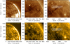 |
Fig. 1. Upper and lower row panels: filament in SDO/AIA 193 Å and 171 Å, respectively. Panels a and d: context of the filament we are considering. Central panels b and e: closer view of the studied filament and the region considered in this study (black box). Panels c and f: filament in AIA 193 Å and 171 Å in the field of view chosen by the rectangular box in (b) and (e). The artificial slits are overplotted on the filament. The slits are labelled by the corresponding numbers. |
2.1. Filament rise and trigger of the oscillations
The event considered in this work consists in a partial and failed eruption of the southern part of the filament and the subsequent LAOs observed in the northern part of the same filament. In this work we focus on the study of the LAOs. It is difficult to study the triggering of the oscillations by the partial eruption because the erupted plasma is very faint and only visible in AIA 304 Å channel (see animated Fig. 3 online). In Fig. 2 and the associated animation, the southern part of the filament, marked with the arrows, can be clearly seen to begin lifting off. The rest of the filament also rise but with a slower rate compared to the southern part. Subsequently, a small portion of the southern part of the filament erupts and a transient brightening due to a change in magnetic field topology is noted, and is outlined by a circle in Fig. 2d. This brightening is also seen in AIA 171 Å and 193 Å data (Fig. 3a at (x, y) = (710, 415)). No signatures of CMEs are seen in the LASCO/C2 field of view, which leads us to conclude that it could be a failed or partial eruption (since only the southern portion of the filament exhibits eruption). Furthermore, the rest of the filament returned to the equilibrium position after a brief liftoff. This might have triggered LAOs due to the large displacement from the mean position. It should be noted that this is mere speculation based on the temporal sequence of the eruption and initiation of the oscillations. In the current study, we focus our analysis on the co-existence of the longitudinal and transverse oscillations and their seismological implications, regardless of how they are triggered.
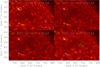 |
Fig. 2. Temporal evolution of the rising filament that probably triggered LAOs. Panels a–c: arrows mark the portion of the filament that started rising before LAOs were triggered. Panel d: transient brightening following the liftoff of the filament is outlined by a circle. An animated version of this figure is available online. |
2.2. Co-existence of longitudinal and transverse oscillations
Figures 3a and corresponding animation online show the filament at the moment of the triggering of the LAO at 16:00 UT. The green arrow shows the direction of the movement of the filament threads towards the left. In Fig. 3b the movement of the filament threads is further towards the left direction at 16:20:09 UT. Figure 3c depicts the rightward movement of the filament threads at 16:40:09 UT and 17:20:09 UT (see Fig. 3d). Subsequently, the direction of the filament motion is again reversed. Furthermore, we also note the signatures of the transverse oscillations in a small bunch of filament threads exhibiting longitudinal oscillations. A detailed analysis is presented in the following sections.
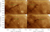 |
Fig. 3. Temporal evolution of the filament in AIA 193 Å in different phases of oscillations. The arrows in green represent the direction of the movement of the filament threads at different instances. An animated version of this figure is available online. |
3. Data analysis and results
3.1. Longitudinal oscillation in filament threads from AIA 171 Å
As described in Sect. 2, we clearly see the oscillations of filament threads. We visually identify the motion of several threads. We place seven artificial horizontal slits labelled from 1 to 7 in Fig. 1c. These slits are placed along the different filament threads to track their motions. These horizontal slits capture the longitudinal oscillations of filament threads. From the artificial slits, we generate time–distance maps, with time in the horizontal axis and distance along the slits in the vertical axis (x − t map). Figures 4a–g show the x − t map produced from slits 1−7, respectively. In all the x − t maps, we observe longitudinal oscillation of dark filament threads. In Figs. 4h–n, points shown in black are the detected intensity minimum points from corresponding x − t maps of Figs. 4a–g, respectively. The red curves in Figs. 4h–n are the fitted damped sinusoidal curves to the detected minimum intensity points with best-fit parameters. The damped sinusoidal curve is represented by the following equation (see, e.g., Aschwanden et al. 1999)
 (1)
(1)
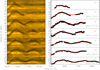 |
Fig. 4. Panels a–g: time–distance diagrams corresponding to slits 1−7, respectively (see Fig. 1n). Panels h–n: minimum intensity position (black asterisks) of the corresponding time–distance map of panels a–g, respectively. The damped exponential sinusoidal fit is depicted by red solid lines. The green dashed lines are drawn to estimate the extent of the damped exponential sinusoidal fit. |
where C is a constant, A is the amplitude, ω is the angular frequency, τ is the damping time, and ϕ is the initial phase of the oscillation. We perform the least square fitting in interactive data language (IDL) using MPFIT.pro (Markwardt 2009).
The best-fit values and the associated errors in the amplitudes, periods (P = 2π/ω), damping time, and velocity amplitudes of the longitudinal oscillations are quoted in Table 1.
Parameters for the damped sinusoidal fitting of longitudinal oscillation in the filament thread in AIA 171 Å.
We discard the data from slit 1 because one-sigma errors in time are very large. This large error is because we capture one half of a period in slit 1. From the table we see that the period ranges from 74 to 86 min. This shows very uniform period values with an average value of 79.83 ± 0.47 min. In contrast, τ values are more dispersed, ranging from 51 to 119 min. The value of damping time is large in comparison to the value reported in Tripathi et al. (2009) but is comparable to the value reported by Luna et al. (2014). The average value of the τ is estimated to be 72.83 ± 2.17 min. The strength of the damping is measured by the parameter τ/P that ranges from 0.59 ± 0.004 to 1.57 ± 0.014. These values indicate a strong damping of the LALOs. The displacement amplitudes, A, have also a large range of values from 8 to 16 Mm and the oscillation velocities, V = ω A, range from 12 to 22 km s−1. The large range of values of A and V indicates that the oscillations in different threads are excited with different energies during the triggering process.
3.2. Longitudinal oscillation in filament threads from AIA 193 Å
We additionally analyze the AIA 193 Å channel using the same seven horizontal slits shown in Fig. 1c. Figure 5 shows the seven time–distance diagrams from the AIA 193 Å data. As in the previous case, black asterisks show the position of the minimum intensity associated to the central location of the threads where the absorption is maximum. We fit the oscillation with Eq. (1) and the resulting parameters are shown in Table 2. The time period varies from 75 to 84 min with an average value of 80.3 ± 0.4 min. The damping time varies in a wide range from 62 to 203 min and the average value of the damping time is estimated to be 97.67 ± 2.74 min. The displacement amplitudes, A, have also a large range of values from 10 to 16 Mm. As in the previous case we discard the fitting parameters from slit 1. The results are similar to the findings from the AIA 171 Å passband. The similarity of results is expected as the geometry remains the same for the two different wavelengths.
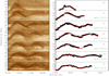 |
Fig. 5. Panels a–g: time distance map of slits 1−7 (see upper right panel of Fig. 1), respectively in AIA 193 Å. Panels h–n: minimum intensity points of corresponding time distance map of panels a–g, respectively, marked with black asterisks. The damped exponential sinusoidal fit is depicted by red solid lines. The green dashed lines are drawn to estimate the extent of the damped exponential sinusoidal fit. |
Parameters for the damped sinusoidal fitting for longitudinal oscillation of filament thread in AIA 193 Å.
The parameters of the longitudinal oscillations are in agreement with the previous findings (Luna et al. 2014; Zhang et al. 2017a) with similar range of periods and damping times. We see little difference in the fitted parameters in AIA 171 Å and 193 Å passbands. Since we are following the cool plasma, the absorption could be slightly different in different channels of AIA which influences the estimation of the best-fit parameters.
3.3. Transverse oscillation in filament threads
The uppermost bunch of threads of the filament in slit 1 also oscillate in the transverse direction over a shorter time span in comparison to longitudinal oscillation. Tracking the transverse motion is difficult due the simultaneous longitudinal displacement of the filament thread. We place a new slit labelled “A” perpendicular to slit 1 (see Figs. 1c and f). We move slit A along slit 1 following the longitudinal movement. In this way we can track the motion in the transverse direction producing the time–distance diagram in slit A using the AIA 171 Å and 193 Å passbands. It should be noted that slit A remains perpendicular to slit 1 at all instances so that spurious oscillations are not detected. From the diagrams in both channels we identify a signature of the oscillation (see Fig. 6). As in the case of the longitudinal oscillations we fit the decaying sinusoidal function (Eq. (1)) to these intensity minimum points.
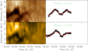 |
Fig. 6. Upper left panel: time–distance map obtained using artificial slit A (see right panels of Fig. 1) in AIA 193 Å data. Lower left panel: similar to the upper left panel but for AIA 171 Å. Black asterisks in upper (and lower) right panel represent the minimum intensity corresponding to the time–distance map shown in the left panels. Overplotted in red is the best-fit exponentially damped sinusoidal curve to the minimum intensity points. |
The parameters of oscillation are shown in Table 3. The transverse oscillations have much smaller amplitudes with displacements of 1.2 and 1.6 Mm in 171 Å and 193 Å, respectively. In contrast, the velocities are comparable to the longitudinal case. The period of oscillations are also considerably smaller than the longitudinal motions. As we discuss in the following section the origin of the transverse oscillation is magnetoacoustic and the restoring force is associated with the magnetic field. The damping is comparable to the period indicating strong damping of the transverse oscillations. However, the measurement of the damping time is not reliable because the filament threads disappear while exhibiting transverse motions as seen in Fig. 6. Transverse oscillations with periods of between 3 and 5 min in the filament threads have been reported in previous studies (Lin et al. 2009; Okamoto et al. 2015). In this study, we find long periods of about 15 min. Since the period of transverse oscillations depends on the length of the fluxtube, long periods in our study indicate that the filament threads might be longer. We discuss this in detail in the following section.
Parameters of sinusoidal fitting for transverse oscillation in the filament thread.
4. Seismology
In this section, we combine the results from our observations with the theoretical models to infer parameters of the prominence. For the longitudinal oscillations, we use the pendulum model by Luna & Karpen (2012) to estimate the radius of curvature of the filament. In the pendulum model, it is assumed that the motion of the plasma is mainly along the dipped field lines that support the prominence against gravity. In these conditions, the gravity is the dominant restoring force and the period depends exclusively on the radius of the curvature of the dips supporting the cool prominence plasma, R, as
 (2)
(2)
where ω is the angular frequency, g0 is the surface gravity of the Sun, and P is the period of the longitudinal oscillation. Using the average value of the period for 171 Å data, P = 79.83 ± 0.47 min, we estimate R = 160 ± 1 Mm. Similarly, using the average periods from the 193 Å data, P = 80.3 ± 0.4, we obtain an identical result: R = 161 ± 1. Both results are similar because the geometry of the filament is the same and independent of the AIA wavelength.
Following Luna & Karpen (2012) and Luna et al. (2014) we estimate the minimum magnetic field by assuming that the magnetic tension in the dipped part of the tubes must be larger than the weight of the threads. With this assumption it is possible to find the following relation:
 (3)
(3)
where B is the magnetic field, ne is the electron number density in cm−3, and P is the period of the oscillation in hours. In the absence of a direct measurement, here we use the typical value of electron number density in the range of 1010–1011 cm−3 (Labrosse et al. 2010). In the estimation of the magnetic field, the density is the most important source of uncertainty as the error in the estimation of the period is much less than the range of density given. Under these conditions Eq. (3) becomes
 (4)
(4)
Using this average value of the longitudinal oscillations we obtain lower limits of the magnetic field of 22.6 ± 11.9 G and 22.8 ± 12.0 G for 171 Å and 193 Å, respectively, which are comparable with the typical values of reported magnetic field (Mackay et al. 2010; Labrosse et al. 2010) by direct means.
In contrast to the LALOs, the transverse oscillations of Sect. 3.3 have a MHD nature. We can therefore study the transverse oscillation applying MHD models. We apply the linear model by Díaz et al. (2002) and Dymova & Ruderman (2005). Figure 7 shows the equilibrium configuration we consider. The prominence thread has a length 2W and density ρp. The thread is embedded in a flux tube of length 2L and density ρe. Both sides of the flux tubes are called evacuated regions and they probably have a density larger than the ambient corona (see models by Dymova & Ruderman 2005; Díaz et al. 2002). The piecewise density along the tube is given by
 (5)
(5)
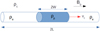 |
Fig. 7. Schematic diagram of the magnetic field and plasma configuration. The blue smaller cylinder represents the flowing thread inside the magnetic tube which is represented by the larger white cylinder. The length of the magnetic tube is 2L and the length of the filament thread is 2W. The density of the thread is ρp, the density of the magnetic tube is ρe, and the density of the outer corona is ρc. The thread is moving along the axis of the tube with velocity v0. |
where z = 0 is the middle point of the tube and z = ±L are the end points of the cylinder. The magnetic field B is along the axis of the cylinder and is the same inside and outside of the cylinder. To study the dynamics of the thread we can assume that the ratio of the width of the thread to its length is very small, which is called thin tube approximation. Terradas et al. (2008) performed a similar seismological analysis. They found that the flow has little influence on the oscillation periods with corrections below the error bar of their observation. For this reason we only studied the special case of negligible flow of the thread. The normal modes of steady non-flowing filament threads were studied by Díaz et al. (2002) and Dymova & Ruderman (2005). The system supports fast and Alfvén waves. The Alfvén waves result in azimuthal (i.e. torsional) motions and so they do not cause displacement of the cylinder axis. In contrast, the kink fast mode leads to displacement of the cylinder axis resulting in transverse oscillation of the filament thread, as we observe. Dymova & Ruderman (2005) provided a simple dispersion relation since they assume the thin tube approximation. The following formula (Eq. (27) in their study) gives the dispersion relation:
 (6)
(6)
where e = ρe/ρc, c = ρp/ρc, l = W/L, and Ω = ωL/vAc, with ω the frequency and vAc the coronal Alfvén speed. The Alfvén speed in the thread plasma and in the evacuated parts of the cylinder are respectively vAp = c−1/2vAc and vAe = e−1/2vAc expressed in terms of the density ratios c and e and  . The frequency of the kink mode is given by the smallest positive root of Eq. (6). This equation establishes a relation between the field strength B, the period P of the transverse oscillation, density contrasts c and e, thread half-length W, and the half-length of the field line L. It is common practice to compute the magnetic field measuring some parameters or assuming their typical values. However, we use the values of B obtained from the seismology of the longitudinal oscillations and therefore we can infer the value of the length of the field line 2L. This is a completely new approach combining both polarizations. From Eq. (6) we obtain the half-length of the flux tube in terms of the rest of the parameters:
![Mathematical equation: $$ \begin{aligned} L= W + \frac{{ v}_{\rm Ac}}{\omega } \sqrt{\frac{2}{1+e}} \tan ^{-1} \left[ \sqrt{\frac{1+e}{1+c}} \cot \left(\frac{\omega W}{{ v}_{\rm Ac}} \sqrt{\frac{1+c}{2}}\right) \right]\cdot \end{aligned} $$](/articles/aa/full_html/2020/01/aa36453-19/aa36453-19-eq8.gif) (7)
(7)
We use the average period of the transverse oscillations, P = 16 min (see Table 3). From Fig. 6 we estimate the thread length to be 2W ∼ 1.5 Mm. From the longitudinal oscillations seismology we estimate B ∼ 11 − 35 G using the pendulum model. Assuming typical coronal electron densities of 108 − 109 cm−3 we obtain that vAc ≥ 759 km s−1 up to several thousand km s−1. However, we assume a maximum value of 1500 km s−1 in agreement with the observations. We assume typical values for c = 100 − 200 (see Mackay et al. 2010; Labrosse et al. 2010) and e identical to the range of values considered by Dymova & Ruderman (2005), that is e = 0.6 − 2. With these ranges of parameters we obtain a range of lengths of the field lines: 2L = 206 − 713 Mm. The range of lengths comprises long to very long field lines. There is no direct measurement of the length of the field lines, but theoretical models assume that the field lines are long: a few hundred thousand kilometres (see Mackay et al. 2010; Luna et al. 2012b; Terradas et al. 2008) and our range of values overlaps the theoretical estimations. Probably, the largest values of the range obtained here by seismology are overestimated due to the uncertainties of the method. This result agrees with the idea that field lines supporting the prominence are very large. Many models of prominence field structure assume a flux rope with many turns. We can assume that the radius of the rope is R. The ratio L/πR then gives an idea of the number of turns of the flux rope. From the seismology we obtain a number smaller than one, suggesting that the field structure consists in a rope with less than one turn.
The damping of the oscillation offers additional information about the prominence and the processes involved on it. Similarly to the oscillation period, assuming a physical damping mechanism we can infer some parameters. In Luna et al. (2012b) and later in Ruderman & Luna (2016) we modelled the damping as a result of the mass accretion associated to the evaporation-condensation process (Mackay et al. 2010). From the approximate Eq. (46) of Ruderman & Luna (2016) we estimate the mass accretion rate to be
 (8)
(8)
with M being the mass of the thread and ̇M = dM/dt. The average longitudinal damping time is τ = 85 min. Using this number we estimate that ̇M/M = 0.025 min−1. However, this number should be considered as a crude estimation because Eq. (46) from Ruderman & Luna (2016) is an approximation.
Luna et al. (2018) found a non-linear behaviour of LAOs using observations. The authors found that the damping time τ depends on the oscillation velocity, V. In Fig. 8 we plot τ as function of the velocity amplitude on each slit. In both panels it seems that there is a trend of reducing τ for increasing V in agreement with previous findings. Zhang et al. (2013) found that the radiative cooling could explain this trend and consequently the damping. The authors found a non-linear relationship between τ and V as τ ∼ Vb with b = −0.3. In Fig. 8 we have over plotted this scaling law. The scaling law of Zhang et al. (2013) seems to follow the trend of the data. From Fig. 8, we note that the scaling law is not very sensitive to b. In addition, we fitted the data with a general form τ = a Vb and we obtained that b ∼ −1.3, which is very different of the scaling law of Zhang et al. (2013). Moreover, Zhang et al. (2013) found a complex dependence of τ on the different parameters of the thread and the field line, such as the thread length, field line length, the geometry of the dip, and the velocity amplitude. The exponents of the parameters are quite large, except for V, indicating that τ is more sensitive to the parameters of the thread and the field lines than V. In the model by Ruderman & Luna (2016) the damping is not directly related to the oscillation velocity. However, events with larger V are associated with violent events, which could produce increased evaporation and consequently stronger damping. More recently, Zhang et al. (2019) found by numerical simulations that wave leakage is an important ingredient of the LAOs damping but in weak field prominences. Additional observational and theoretical efforts are necessary to determine the combination of mechanisms responsible for the strong LAO damping and their applicability to seismology.
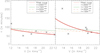 |
Fig. 8. Left panel: variation of damping time (τ) with velocity (v) of the oscillation in AIA 171 Å. Right panel: similar to the left but for AIA 193 Å. The black asterisks represent the observed data. A non-linear curve given by the relation τ ∼ a Vb is fitted to the data. Curves with different exponents and constants are overplotted in different colours and line styles. The curve in solid red in the left (right) panel represents the best-fit curve with a and b (in the relation τ ∼ a Vb) of 450 (3657) and −0.7 (−1.3), respectively. |
5. Summary and conclusions
In this work, we report simultaneous longitudinal and transverse oscillation in the same filament threads for the first time. The event occurred in a large filament located in the northwest quadrant of the solar disk on July 7, 2017. Triggering of the LAOs is associated to the failed eruption of the filament. The filament starts to rise around 13 UT. The eruption fails and the filament falls to the equilibrium position. This produces oscillations of part of the cool plasma of the filament. The oscillations are mainly longitudinal but one thread also oscillates in the transverse direction to the local field. We use the time–distance technique to analyse the oscillations and obtain the oscillation parameters in both AIA 171 Å and 193 Å channels. Both channels show identical oscillations. The periods obtained are in the range of 75−86 min with an average value of 80 min. The velocities of the oscillations are in the range of 12−23 km s−1 and therefore these are LALOs. The oscillations are strongly damped with damping times comparable to the oscillation period. The transverse oscillations in one of the threads have a considerably smaller period of 16 min, an average velocity amplitude of 9 km s−1in both channels, and an average damping time of 24 min.
We applied a seismological technique to both oscillation polarizations. For the longitudinally oscillating case, we used the pendulum model and determined the radius of the curvature of the magnetic dips hosting the prominence, R, and the minimum field strength, B, required to support the mass against gravity. The resulting average values in the seven slits are R = 160 Mm and B = 23 ± 12 G. For the transverse oscillations the restoring force is associated to the magnetic Lorentz force. In a novel way we combine the magnetic field obtained with the longitudinal oscillations with the dispersion relation of the transverse modes to obtain the length of the field lines hosting the prominence. The lengths of these field lines are in the range of 206−713 Mm.
We applied seismological techniques in a novel way that allowed us to measure the strength, the curvature of the dips, and the length of the magnetic field lines supporting the prominence. Our findings suggest that the prominence structure consists in a flux rope with few turns, probably less than one.
Movies
Movie of Fig. 2 Access Supplementary Material
Movie of Fig. 3 Access Supplementary Material
Acknowledgments
VP was supported by the GOA-2015-014 (KU Leuven) and the European Research Council (ERC) under the European Union’s Horizon 2020 research and innovation programme (grant agreement No 724326). M. L. acknowledges the support by the Spanish Ministry of Economy and Competitiveness (MINECO) through projects AYA2014-55078-P and under the 2015 Severo Ochoa Program MINECO SEV-2015-0548. M. L. and V. P. acknowledge support from the International Space Science Institute (ISSI), Bern, Switzerland to the International Team 413 “Large-Amplitude Oscillations as a Probe of Quiescent and Erupting Solar Prominences” (P.I. M. Luna). DB and VP acknowledge the support from the ISSI-Beijing for the formation of the international team titled “The eruption of solar filaments and the associated mass and energy transport” and its activities. R. M. acknowledges the support of United Grants Commission (UGC) and Center of Excellence in Space Sciences India (CESSI), IISER KOLKATA. We also thank the anonymous referee for careful reading and constructive suggestions.
References
- Andries, J., Arregui, I., & Goossens, M. 2005, ApJ, 624, L57 [NASA ADS] [CrossRef] [Google Scholar]
- Arregui, I. 2012, Astrophys. Space Sci. Proc., 33, 159 [NASA ADS] [CrossRef] [Google Scholar]
- Arregui, I., & Ballester, J. L. 2011, Space Sci. Rev., 158, 169 [NASA ADS] [CrossRef] [Google Scholar]
- Arregui, I., Oliver, R., & Ballester, J. L. 2018, Liv. Rev. Sol. Phys., 15, 3 [CrossRef] [Google Scholar]
- Aschwanden, M. J., Fletcher, L., Schrijver, C. J., & Alexander, D. 1999, ApJ, 520, 880 [NASA ADS] [CrossRef] [Google Scholar]
- Chandra, R., Schmieder, B., Mandrini, C. H., et al. 2011, Sol. Phys., 269, 83 [NASA ADS] [CrossRef] [Google Scholar]
- Chen, J., Xie, W., Zhou, Y., et al. 2017, Ap&SS, 362, 165 [NASA ADS] [CrossRef] [Google Scholar]
- Díaz, A. J., Oliver, R., & Ballester, J. L. 2002, ApJ, 580, 550 [NASA ADS] [CrossRef] [Google Scholar]
- Dymova, M. V., & Ruderman, M. S. 2005, Sol. Phys., 229, 79 [NASA ADS] [CrossRef] [Google Scholar]
- Eto, S., Isobe, H., Narukage, N., et al. 2002, PASJ, 54, 481 [NASA ADS] [CrossRef] [Google Scholar]
- Gilbert, H. R., Holzer, T. E., Burkepile, J. T., & Hundhausen, A. J. 2000, ApJ, 537, 503 [NASA ADS] [CrossRef] [Google Scholar]
- Gilbert, H. R., Daou, A. G., Young, D., Tripathi, D., & Alexander, D. 2008, ApJ, 685, 629 [NASA ADS] [CrossRef] [Google Scholar]
- Gopalswamy, N., Shimojo, M., Lu, W., et al. 2003, ApJ, 586, 562 [NASA ADS] [CrossRef] [Google Scholar]
- Hershaw, J., Foullon, C., Nakariakov, V. M., & Verwichte, E. 2011, A&A, 531, A53 [NASA ADS] [CrossRef] [EDP Sciences] [Google Scholar]
- Hyder, C. L. 1966, ZAp, 63, 78 [Google Scholar]
- Isobe, H., & Tripathi, D. 2006, A&A, 449, L17 [NASA ADS] [CrossRef] [EDP Sciences] [Google Scholar]
- Isobe, H., Tripathi, D., Asai, A., & Jain, R. 2007, Sol. Phys., 246, 89 [NASA ADS] [CrossRef] [Google Scholar]
- Jing, J., Lee, J., Spirock, T. J., et al. 2003, ApJ, 584, L103 [NASA ADS] [CrossRef] [Google Scholar]
- Jing, J., Yurchyshyn, V. B., Yang, G., Xu, Y., & Wang, H. 2004, ApJ, 614, 1054 [NASA ADS] [CrossRef] [Google Scholar]
- Jing, J., Lee, J., Spirock, T. J., & Wang, H. 2006, Sol. Phys., 236, 97 [NASA ADS] [CrossRef] [Google Scholar]
- Labrosse, N., Heinzel, P., Vial, J.-C., et al. 2010, Space Sci. Rev., 151, 243 [Google Scholar]
- Lemen, J. R., Title, A. M., Akin, D. J., et al. 2012, Sol. Phys., 275, 17 [NASA ADS] [CrossRef] [Google Scholar]
- Li, T., & Zhang, J. 2012, ApJ, 760, L10 [NASA ADS] [CrossRef] [Google Scholar]
- Lin, Y., Soler, R., Engvold, O., et al. 2009, ApJ, 704, 870 [NASA ADS] [CrossRef] [Google Scholar]
- Liu, R., Liu, C., Xu, Y., et al. 2013, ApJ, 773, 166 [Google Scholar]
- Luna, M., & Karpen, J. 2012, ApJ, 750, L1 [NASA ADS] [CrossRef] [Google Scholar]
- Luna, M., Díaz, A. J., & Karpen, J. 2012a, ApJ, 757, 98 [NASA ADS] [CrossRef] [Google Scholar]
- Luna, M., Karpen, J. T., & Devore, C. R. 2012b, ApJ, 746, 30 [NASA ADS] [CrossRef] [Google Scholar]
- Luna, M., Knizhnik, K., Muglach, K., et al. 2014, ApJ, 785, 79 [NASA ADS] [CrossRef] [Google Scholar]
- Luna, M., Díaz, A. J., Oliver, R., Terradas, J., & Karpen, J. 2016a, A&A, 593, A64 [NASA ADS] [CrossRef] [EDP Sciences] [Google Scholar]
- Luna, M., Terradas, J., Khomenko, E., Collados, M., & Vicente, A. D. 2016b, ApJ, 817, 157 [NASA ADS] [CrossRef] [Google Scholar]
- Luna, M., Su, Y., Schmieder, B., Chandra, R., & Kucera, T. A. 2017, ApJ, 850, 143 [NASA ADS] [CrossRef] [Google Scholar]
- Luna, M., Karpen, J., Ballester, J. L., et al. 2018, ApJS, 236, 35 [NASA ADS] [CrossRef] [Google Scholar]
- Mackay, D. H., Karpen, J. T., Ballester, J. L., Schmieder, B., & Aulanier, G. 2010, Space Sci. Rev., 151, 333 [NASA ADS] [CrossRef] [Google Scholar]
- Markwardt, C. B. 2009, in Astronomical Data Analysis Software and Systems XVIII, eds. D. A. Bohlender, D. Durand, & P. Dowler, ASP Conf. Ser., 411, 251 [NASA ADS] [Google Scholar]
- Moreton, G. E., & Ramsey, H. E. 1960, PASP, 72, 357 [Google Scholar]
- Nakariakov, V. M., & Verwichte, E. 2005, Liv. Rev. Sol. Phys., 2, 3 [Google Scholar]
- Okamoto, T. J., Nakai, H., Keiyama, A., et al. 2004, ApJ, 608, 1124 [NASA ADS] [CrossRef] [Google Scholar]
- Okamoto, T. J., Antolin, P., De Pontieu, B., et al. 2015, ApJ, 809, 71 [NASA ADS] [CrossRef] [Google Scholar]
- Oliver, R., & Ballester, J. L. 2002, Sol. Phys., 206, 45 [NASA ADS] [CrossRef] [Google Scholar]
- Pant, V., Srivastava, A. K., Banerjee, D., et al. 2015, Res. Astron. Astrophys., 15, 1713 [NASA ADS] [CrossRef] [Google Scholar]
- Pant, V., Mazumder, R., Yuan, D., et al. 2016, Sol. Phys., 291, 3303 [NASA ADS] [CrossRef] [Google Scholar]
- Pintér, B., Jain, R., Tripathi, D., & Isobe, H. 2008, ApJ, 680, 1560 [NASA ADS] [CrossRef] [Google Scholar]
- Pouget, G., Bocchialini, K., & Solomon, J. 2006, in SOHO-17. 10 Years of SOHO and Beyond, ESA Spec. Publ., 617, 141 [Google Scholar]
- Ramsey, H. E., & Smith, S. F. 1966, AJ, 71, 197 [NASA ADS] [CrossRef] [Google Scholar]
- Ruderman, M. S., & Luna, M. 2016, A&A, 591, A131 [NASA ADS] [CrossRef] [EDP Sciences] [Google Scholar]
- Shen, Y., Liu, Y. D., Chen, P. F., & Ichimoto, K. 2014, ApJ, 795, 130 [NASA ADS] [CrossRef] [Google Scholar]
- Terradas, J., Arregui, I., Oliver, R., & Ballester, J. L. 2008, ApJ, 678, L153 [NASA ADS] [CrossRef] [Google Scholar]
- Tripathi, D., Isobe, H., & Jain, R. 2009, Space Sci. Rev., 149, 283 [NASA ADS] [CrossRef] [Google Scholar]
- Vršnak, B., Veronig, A. M., Thalmann, J. K., & Žic, T. 2007, A&A, 471, 295 [NASA ADS] [CrossRef] [EDP Sciences] [Google Scholar]
- Zhang, Q. M., & Ji, H. S. 2018, ApJ, 860, 113 [NASA ADS] [CrossRef] [Google Scholar]
- Zhang, Q. M., Chen, P. F., Xia, C., & Keppens, R. 2012, A&A, 542, A52 [NASA ADS] [CrossRef] [EDP Sciences] [Google Scholar]
- Zhang, Q. M., Chen, P. F., Xia, C., Keppens, R., & Ji, H. S. 2013, A&A, 554, A124 [NASA ADS] [CrossRef] [EDP Sciences] [Google Scholar]
- Zhang, Q. M., Ning, Z. J., Guo, Y., et al. 2015, ApJ, 805, 4 [NASA ADS] [CrossRef] [Google Scholar]
- Zhang, Q. M., Li, T., Zheng, R. S., Su, Y. N., & Ji, H. S. 2017a, ApJ, 842, 27 [NASA ADS] [CrossRef] [Google Scholar]
- Zhang, Q. M., Li, D., & Ning, Z. J. 2017b, ApJ, 851, 47 [NASA ADS] [CrossRef] [Google Scholar]
- Zhang, L. Y., Fang, C., & Chen, P. F. 2019, ApJ, 884, 74 [NASA ADS] [CrossRef] [Google Scholar]
All Tables
Parameters for the damped sinusoidal fitting of longitudinal oscillation in the filament thread in AIA 171 Å.
Parameters for the damped sinusoidal fitting for longitudinal oscillation of filament thread in AIA 193 Å.
Parameters of sinusoidal fitting for transverse oscillation in the filament thread.
All Figures
|
Fig. 1. Upper and lower row panels: filament in SDO/AIA 193 Å and 171 Å, respectively. Panels a and d: context of the filament we are considering. Central panels b and e: closer view of the studied filament and the region considered in this study (black box). Panels c and f: filament in AIA 193 Å and 171 Å in the field of view chosen by the rectangular box in (b) and (e). The artificial slits are overplotted on the filament. The slits are labelled by the corresponding numbers. |
| In the text | |
|
Fig. 2. Temporal evolution of the rising filament that probably triggered LAOs. Panels a–c: arrows mark the portion of the filament that started rising before LAOs were triggered. Panel d: transient brightening following the liftoff of the filament is outlined by a circle. An animated version of this figure is available online. |
| In the text | |
|
Fig. 3. Temporal evolution of the filament in AIA 193 Å in different phases of oscillations. The arrows in green represent the direction of the movement of the filament threads at different instances. An animated version of this figure is available online. |
| In the text | |
|
Fig. 4. Panels a–g: time–distance diagrams corresponding to slits 1−7, respectively (see Fig. 1n). Panels h–n: minimum intensity position (black asterisks) of the corresponding time–distance map of panels a–g, respectively. The damped exponential sinusoidal fit is depicted by red solid lines. The green dashed lines are drawn to estimate the extent of the damped exponential sinusoidal fit. |
| In the text | |
|
Fig. 5. Panels a–g: time distance map of slits 1−7 (see upper right panel of Fig. 1), respectively in AIA 193 Å. Panels h–n: minimum intensity points of corresponding time distance map of panels a–g, respectively, marked with black asterisks. The damped exponential sinusoidal fit is depicted by red solid lines. The green dashed lines are drawn to estimate the extent of the damped exponential sinusoidal fit. |
| In the text | |
|
Fig. 6. Upper left panel: time–distance map obtained using artificial slit A (see right panels of Fig. 1) in AIA 193 Å data. Lower left panel: similar to the upper left panel but for AIA 171 Å. Black asterisks in upper (and lower) right panel represent the minimum intensity corresponding to the time–distance map shown in the left panels. Overplotted in red is the best-fit exponentially damped sinusoidal curve to the minimum intensity points. |
| In the text | |
|
Fig. 7. Schematic diagram of the magnetic field and plasma configuration. The blue smaller cylinder represents the flowing thread inside the magnetic tube which is represented by the larger white cylinder. The length of the magnetic tube is 2L and the length of the filament thread is 2W. The density of the thread is ρp, the density of the magnetic tube is ρe, and the density of the outer corona is ρc. The thread is moving along the axis of the tube with velocity v0. |
| In the text | |
|
Fig. 8. Left panel: variation of damping time (τ) with velocity (v) of the oscillation in AIA 171 Å. Right panel: similar to the left but for AIA 193 Å. The black asterisks represent the observed data. A non-linear curve given by the relation τ ∼ a Vb is fitted to the data. Curves with different exponents and constants are overplotted in different colours and line styles. The curve in solid red in the left (right) panel represents the best-fit curve with a and b (in the relation τ ∼ a Vb) of 450 (3657) and −0.7 (−1.3), respectively. |
| In the text | |
Current usage metrics show cumulative count of Article Views (full-text article views including HTML views, PDF and ePub downloads, according to the available data) and Abstracts Views on Vision4Press platform.
Data correspond to usage on the plateform after 2015. The current usage metrics is available 48-96 hours after online publication and is updated daily on week days.
Initial download of the metrics may take a while.