| Issue |
A&A
Volume 633, January 2020
|
|
|---|---|---|
| Article Number | A28 | |
| Number of page(s) | 11 | |
| Section | Planets and planetary systems | |
| DOI | https://doi.org/10.1051/0004-6361/201935958 | |
| Published online | 03 January 2020 | |
MuSCAT2 multicolour validation of TESS candidates: an ultra-short-period substellar object around an M dwarf
1
Instituto de Astrofísica de Canarias (IAC),
38200
La Laguna,
Tenerife,
Spain
e-mail: This email address is being protected from spambots. You need JavaScript enabled to view it.
2
Departamento de Astrofísica, Universidad de La Laguna (ULL),
38206 La Laguna,
Tenerife,
Spain
3
Centro de Astrobiologia (CSIC-INTA),
Carretera de Ajalvir km 4,
28850
Torrejon de Ardoz,
Madrid,
Spain
4
Department of Astronomy, The University of Tokyo,
7-3-1 Hongo,
Bunkyo-ku,
Tokyo
113-0033,
Japan
5
Astrobiology Center,
2-21-1 Osawa,
Mitaka,
Tokyo
181-8588,
Japan
6
Japan Science and Technology Agency,
PRESTO,
7-3-1 Hongo,
Bunkyo-ku,
Tokyo
113-0033,
Japan
7
National Astronomical Observatory of Japan,
2-21-1 Osawa,
Mitaka,
Tokyo
181-8588,
Japan
8
Department of Earth and Planetary Science, The University of Tokyo,
Tokyo,
Japan
9
Rheinisches Institut für Umweltforschung an der Universität zu Köln,
Abteilung Planetenforschung,
Aachener Str. 209,
50931
Köln,
Germany
10
European Space Agency,
ESTEC,
Keplerlaan 1,
2201
AZ Noordwijk,
The Netherlands
11
Department of Physics, Kyoto Sangyo University,
Kyoto,
Japan
12
Department of Physics and Kavli Institute for Astrophysics and Space Research, Massachusetts Institute of Technology,
Cambridge,
MA
02139,
USA
13
Center for Astrophysics ∣ Harvard & Smithsonian,
60 Garden Street,
Cambridge,
MA
02138,
USA
14
Department of Physics and Astronomy, Vanderbilt University,
Nashville,
TN
37235,
USA
15
American Association of Variable Star Observers,
49 Bay State Road,
Cambridge,
MA
02138,
USA
16
Astronomy and Physics, Wesleyan University, Middletown, CT, USA, MIT,
Cambridge,
MA,
USA
17
Departamento de Astronomía, Universidad de Chile,
Camino El Observatorio 1515,
Las Condes,
Santiago,
Chile
18
NASA Ames Research Center,
Moffett Field,
CA
94035,
USA
19
SETI Institute,
189 Bernardo Avenue, Suite 100,
Mountain View,
CA
94043,
USA
20
NASA Goddard Space Flight Center,
Greenbelt,
MD
20771,
USA
21
Department of Aeronautics and Astronautics, Massachusetts Institute of Technology,
Cambridge,
MA
02139,
USA
22
Department of Earth, Atmospheric, and Planetary Sciences, Massachusetts Institute of Technology,
Cambridge,
MA
02139,
USA
23
Department of Astrophysical Sciences, Princeton University,
Princeton,
NJ
08544,
USA
Received:
25
May
2019
Accepted:
7
November
2019
Abstract
Context. We report the discovery of TOI 263.01 (TIC 120916706), a transiting substellar object (R = 0.87 RJup) orbiting a faint M3.5 V dwarf (V = 18.97) on a 0.56 d orbit.
Aims. We setout to determine the nature of the Transiting Exoplanet Survey Satellite (TESS) planet candidate TOI 263.01 using ground-based multicolour transit photometry. The host star is faint, which makes radial-velocity confirmation challenging, but the large transit depth makes the candidate suitable for validation through multicolour photometry.
Methods. Our analysis combines three transits observed simultaneously in r′, i′, and zs bands usingthe MuSCAT2 multicolour imager, three LCOGT-observed transit light curves in g′, r′, and i′ bands, a TESS light curve from Sector 3, and a low-resolution spectrum for stellar characterisation observed with the ALFOSC spectrograph. We modelled the light curves with PYTRANSIT using a transit model that includes a physics-based light contamination component, allowing us to estimate the contamination from unresolved sources from the multicolour photometry. Using this information we were able to derive the true planet–star radius ratio marginalised over the contamination allowed by the photometry.Combining this with the stellar radius, we were able to make a reliable estimate of the absolute radius of the object.
Results. The ground-based photometry strongly excludes contamination from unresolved sources with a significant colour difference to TOI 263. Furthermore, contamination from sources of the same stellar type as the host is constrained to levels where the true radius ratio posterior has a median of 0.217 and a 99 percentile of0.286. The median and maximum radius ratios correspond to absolute planet radii of 0.87 and 1.41 RJup, respectively,which confirms the substellar nature of the planet candidate. The object is either a giant planetor a brown dwarf (BD) located deep inside the so-called “brown dwarf desert”. Both possibilities offer a challenge to current planet/BD formation models and make TOI 263.01 an object that merits in-depth follow-up studies.
Key words: stars: individual: TIC 120916706 / planets and satellites: general / methods: statistical / techniques: photometric
© ESO 2019
1 Introduction
The Transiting Exoplanet Survey Satellite (TESS) mission is expected to discover thousands of transiting exoplanet candidates orbiting bright nearby stars. However, since various astrophysical phenomena can lead to a photometric signal mimicking an exoplanet transit (Cameron 2012), only a fraction of the candidates will be legitimate planets (Moutou et al. 2009; Almenara et al. 2009; Santerne et al. 2012; Fressin et al. 2013), and the true nature of the candidates needs to be resolved by follow-up observations (Cabrera et al. 2017; Mullally et al. 2018). A mass estimate based on radial velocity (RV) measurements offers the most reliable way for candidate confirmation, but RV observations are practical only for bright, slowly rotating host stars. Alternative validation methods need to be applied for candidates around hosts not amenable to RV follow-up.
We report the discovery of TOI 263.01 (TIC 120916706), a transiting substellar object (0.44 RJup < R < 1.41 RJup) orbiting a faint M dwarf (M⋆ = 0.4 ± 0.1 M⊙ , R⋆ = 0.405 ± 0.077 R⊙ , V = 18.97 ± 0, 2) on a 0.56 d orbit. The object was originally identified in the TESS Sector 3 photometry by the TESS Science Processing Operations Center (SPOC) pipeline (Jenkins et al. 2016), and was later followed up from the ground using multicolour transit photometry and low-resolution spectroscopy. The planet candidate passes all the SPOC Data Validation tests (Twicken et al. 2018), and is either a planet or a brown dwarf located in a very sparsely populated region in substellar object period-radius space.
The faintness of TOI 263 (see Table 1) makes the planet candidate challenging for RV confirmation1. However, multicolour transit photometry can be used to validate the nature of the candidate (Rosenblatt 1971; Drake 2003; Tingley 2004; Tingley et al. 2014; Parviainen et al. 2019).
Transiting planet candidate validation through multicolour transit photometry works by constraining the light contamination from unresolved sources (blending). This allows us to detect blended eclipsing binaries and, combined with a physics-based light contamination model, allows us to estimate uncontaminated radius ratio (true radius ratio) of the transiting object. Combining the true radius ratio estimate with an estimate of the stellar radius yields the absolute radius of the transiting object, and if the absolute radius is securely below the theoretical radius limit for a brown dwarf, the candidate can be considered a planet.
Our analysis is based on three nights of simultaneous ground-based multicolour transit photometry in r′, i′, and zs bands taken with MuSCAT2 multicolour imager (Narita et al. 2019) installed in the 1.5 m Telescopio Carlos Sanchez (TCS) in the Teide Observatory, three transit light curves observed in g′, r′, and i′ bands with the SINISTRO cameras in the 1 m LCOGT telescopes, and a TESS light curve from Sector 3. The analysis uses a light contamination model included in PYTRANSIT v2, and yields the posterior densities for the model parameters that define the geometry and orbit of the candidate, as well as an estimate of the true radius ratio in the presence of possible light contamination from blended sources, or from the transiting object itself2.
The analysis code is available with the data and supplementary material (such as per-dataset analyses and posterior sensitivity tests) from GitHub3, and we encourage anyone interested to scrutinise the code (and the underlying assumptions) to ensure its integrity.
TOI 263 identifiers, coordinates, properties, and magnitudes.
2 Observations
2.1 TESS photometry
TESS observed TOI 263.01 during Sector 3 for 27 days covering 35 transits with a two-minute cadence. We chose to use the Simple Aperture Photometry (SAP) light curves produced by the SPOC pipeline (Jenkins et al. 2016) over the Presearch Data Conditioning (PDC) light curves because the noise in the light curve is dominated by the photon noise (PDC adds some noise but did not improve the photometry in this case) and because the PDC process removes the PDC-estimated flux contamination. The latter can introduce bias into our contamination estimation if the PDC contamination is overestimated because we do not allow for “negative contamination”.
The TESS photometry used in the analysis consists of 35 subsets spanning 2.4 h centred around each transit based on the linear ephemeris, and each subset was normalised to its median out-of-transit (OOT) level assuming a transit duration of 0.96 h. The photometry has an average point-to-point (ptp) scatter of 65 ppt (65 000 ppm). We do not detrend the photometry, but include a free baseline level and white noise standard deviation as per-transit free parameters in the analyses. We also experimented with higher order polynomial baseline models and Gaussian Process-based likelihood models, as mentioned later in Sect. 4, but these did not change the parameter posteriors due to the dominance of photon noise.
2.2 MuSCAT2 photometry
We observed two full and one partial transits of TOI 263.01 with the MuSCAT2 multicolour imager (Narita et al. 2019) installed in Telescopio Carlos Sanchez (TCS) in the Teide Observatory on the nights of 18.12.2018, 19.12.2018, and 02.01.2019. MuSCAT2 is a four-colour instrument consisting of four independently controlled CCDs, but one of the CCDs was under maintenance, and the observations were carried out simultaneously in three colours (r′, i′, zs).
The exposure times for the first night were 30, 60, and 60 s; for the second night 30, 90, and 90 s; and for the last night 60, 60, and 60 s, with white noise estimates of 47, 14, 13, 47, 14, 12, 13, 8, and 8 ppt, respectively. The r′ -band was used for guiding and had a short exposure time during the first two nights (which combined with the redness of TOI 263 explains the high white noise level). A longer exposure time was used for the guiding channel on the third night without any negative effects on the photometry. On the contrary, the last night had the best observing conditions and the quality of the photometry is significantly higher than on the first two nights.
The photometry was carried out using standard aperture photometry calibration and reduction steps with a dedicated MuSCAT2 photometry pipeline. The pipeline calculates aperture photometry for a set of comparison stars and photometry aperture sizes (see Fig. 1), and creates the final relative light curves via global optimisation of the posterior density for a model consisting of a transit model, apertures, comparison stars, and a linear baseline model with the airmass, seeing, x- and y-centroid shifts, and the sky level as covariates (that is, the best comparison stars and aperture sizes are also optimised).
The resulting light curves are stored as fits files with the raw and reduced photometry, best-fitting transit model, best-fitting baseline model, the covariates, and the covariate coefficients producing the baseline model included in binary tables. The MuSCAT2 pipeline reduction also yields posterior estimates for the transit model, including a contamination estimate based on the approach described in Sect. 4.2 and detailed further in Parviainen et al. (2019). While the final analysis presented in Sect. 4 combines all the photometric data into a joint analysis, these estimates are important as a consistency check to study the night-to-night variations in the parameters of interest.
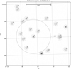 |
Fig. 1 MuSCAT2 field observed in i′ band with TOI 263 marked with a “0” and the rest of the stars numbered from brightest to faintest. The circles show the apertures used to extract the photometry, and the two outermost circles mark the annulus used to measure the sky level. The dotted circle marks a 2′ circle centred around TOI 263. |
2.3 LCOGT photometry
Three full transits of TOI 263.01 were observed using the Las Cumbres Observatory Global Telescope (LCOGT) 1 m network (Brown et al. 2013)in i′, r′, and g′ bands on the nights of 13.12.2018, 26.12.2018, and 21.01.2019, respectively, as part of the TESS Follow-up Observing Program (TFOP). We used the TESS Transit Finder, which is a customised version of the Tapir software package (Jensen & Eric 2013), to schedule our transit observations. The g′ and i′ transits were observed from the LCOGT node at South Africa Astronomical Observatory and used 200 and 100 s exposures respectively. The r′ transit was observed from the LCOGT node at Cerro Tololo Inter-American Observatory and used 120 s exposures. The telescopes are equipped with 4096 × 4096 LCO SINISTRO cameras with an image scale of 0.′′389 pixel−1 resulting in a 26′ × 26′ field of view.
The images were calibrated by the standard LCOGT BANZAI pipeline and the photometric data were extracted using the AstroImageJ (AIJ) software package (Collins et al. 2017). Circular apertures with radii of 5, 8, and 8 pixels were used to extract differential photometry in the g′, r′, and i′ -bands resulting in estimated white noise of 28-ppt, 7.55 ppt, and 7.55 ppt, respectively. The images have stellar point-spread-functions (PSFs) with FWHM ranging from 1.′′2 to 1.′′8. The nearest star in the Gaia DR2 catalogue is 21.′′2 to the north of TOI 263, so the photometric apertures are not contaminated with significant flux from known nearby stars.
2.4 ALFOSC spectroscopy
We used low-resolution optical spectrum observed using the Alhambra Faint Object Spectrograph and Camera (ALFOSC) of the 2.5-m Nordic Optical Telescope (NOT) on Roque de los Muchachos Observatory (La Palma) to obtain the basic stellar properties of TOI 263. A total of two spectra with on-source exposure times of 1800 s each were obtained on 2019 January 21. ALFOSC is equipped with an E2V 2048 × 2048 CCD detector with a pixel size of 0.′′2138 projected onto the sky. We used the grism number 5 and a long slit width of 1.′′0, which yield spectra between 5000 and 9200 Å with a spectral resolution of 16.6 Å (R = 430 at 7100 Å). Seeing conditions and sky transparency were adequate for carrying out spectroscopic observations. TOI 263 was observed at parallactic angle and at a relatively low airmass of 1.7.
ALFOSC raw frames were reduced following standard procedures at optical wavelengths: bias subtraction,flat-fielding using dome flats, and optimal extraction using appropriate packages within the IRAF4 environment. Wavelength calibration was performed using He I and Ne I arc lines observed immediately after the acquisition of the target data. The instrumental response was corrected using observations of the spectrophotometric standard star GJ 246 (a white dwarf) taken with exactly the same instrumental configuration as our target on 2019 February 4. Unfortunately, the standard was observed at the low airmass of 1.2; we cannot use it for removing the telluric contribution from the target data. The two individual spectra of TOI 263 were combined and the final spectrum, depicted in Fig. 2, is of sufficiently good quality (S∕N > 150) for a proper spectral classification.
3 Stellar characterisation
The object TOI 263 shows strong absorption due to TiO all over the ALFOSC spectrum while VO is not present, and the observed pseudo-continuum increases toward long wavelengths, all of which clearly indicates an early- to mid-M spectral type. We employed the spectroscopic standard stars defined in Table 3 by Alonso-Floriano et al. (2015) to derive an M3.5 V spectral type for TOI 263, since Luyten’s star (also depicted in Fig. 2) provides thebest match to the ALFOSC data. The spectra of Alonso-Floriano et al. (2015) are of slightly higher resolution than our data (by a factor of 3.5); however the comparison is feasible given the overlapping wavelength coverage. The different spectral resolution does not affect the spectral typing of TOI 263. We estimated an error of ±0.5 subtypes for our classification. The object TOI 263 shows Hα in emission with a pseudo-equivalent width (pEW) of − 3.9 ± 0.2 Å. This width is typical among field M3–M4-type stars (see Fig. 8 of Alonso-Floriano et al. 2015) and lies well below the threshold defined for accreting M dwarfs (see Navascus & Martín 2003), thus indicating that TOI 263 is quite likely not a very young star in the solar neighbourhood. Given the low spectral resolution of our data, we could not assess the surface gravity of the star with precision; however, the Na I resonance doublet at ~8195 Å, which is a well-known age indicator for M dwarfs, is clearly detected with pEW = 3.6 ± 0.2 Å in TOI 263. This value is typical of field, high-gravity M3–M4 dwarfs (see Table 5 by Martin et al. 1996, see also Schlieder et al. 2012), which suggests that TOI 263 likely has the “age of the field”, that is between ≈0.5 and ≈9 Gyr. Similarly to the surface gravity, the metallicity of the star cannot be addressed quantitatively using the ALFOSC data. However, there is no strong absorption due to hydrides in the observed optical spectrum, suggesting that TOI 263 likely has a near solar chemical composition (Kirkpatrick et al. 2014, and the references therein).
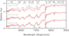 |
Fig. 2 ALFOSC spectrum of TOI 263 with a resolution of 16.6 Å is plotted as a red line. It is compared to the spectra of three spectral standard stars from the catalogue of Alonso-Floriano et al. (2015), which are shown with a black line: GJ 2066 (J08161+013, M2V), Luyten’s star (J07274+052, M3.5V), and V1352 Ori (J05421+124, M4V). All spectra are normalised to 1.0 at the red continuum of the subordinate Na I lines, and are shifted vertically by 1.0 for clarity. The strongest molecular and atomic features are indicated on the top. The strongest telluric oxygen features are also labelled. |
4 Transit light-curve analysis
4.1 Overview
We first analysed each photometric dataset (MuSCAT2, TESS, and LCOGT) independently, and then combined them for a joint analysis. We do not detail the independent analyses here, but make them available online as Jupyter notebooks in GitHub.
The final dataset consists of the 35 transits in the TESS data from Sector 3, three transits observed simultaneously in three passbands with MuSCAT2, and three transits observed in three passbands with the LCOGT telescopes. This sums up to five passbands, 41 transits, and 47 light curves. The analysis follows standard steps for Bayesian parameter estimation (Parviainen 2018). First, we construct a flux model with the aim of reproducing the transit and the light curve systematic errors. Next, we define a noise model to explain the stochastic variability in the observations not explained by the deterministic flux model. Combining the flux model, the noise model, and the observations gives us the likelihood. Finally, we define the priors on the model parameters, after which we estimate the joint parameter posterior distribution using Markov chain Monte Carlo (MCMC) sampling.
The posterior estimation begins with a global optimisation run using Differential Evolution (Storn & Price 1997; Price et al. 2005)that results with a population of parameter vectors clumped close to the global posterior mode. This parameter vector population is then used as a starting population for the MCMC sampling with EMCEE, and the sampling is carried out until a suitable posterior sample has been obtained (Parviainen 2018).
The analyses were carried out with a custom Python code based on PYTRANSIT v25 (Parviainen 2015; Parviainen et al. 2019), which includes a physics-based contamination model based on the PHOENIX-calculated stellar spectrum library by Husser et al. (2013). The limb darkening computations were carried out with LDTK 6 (Parviainen & Aigrain 2015), and MCMC sampling was carried out with EMCEE (Foreman-Mackey et al. 2013; Goodman & Weare 2010).
The code relies on the existing PYTHON packages for scientific computing and astrophysics: SCIPY, NUMPY (van der Walt et al. 2011), ASTROPY (Astropy Collaboration 2013), PHOTUTILS (Bradley et al. 2019), ASTROMETRY.NET (Lang et al. 2010), IPYTHON (Perez & Granger 2007), PANDAS (Mckinney 2010), XARRAY (Hoyer & Hamman 2017), MATPLOTLIB (Hunter 2007), and SEABORN. All the code for the analyses presented in this paper is available from GitHub as Python code and Jupyter notebooks7.
4.2 Contaminated transit model
The candidate validation is based on the true planetary radius estimate obtained by modelling the multicolour transit photometry with a transit model that includes a physics-based light contamination component. The contamination is parametrised by the effective temperatures of the host and the contaminant, and the amount of contamination in some reference passband (TEff,H, TEff,C, and c) (Parviainen et al. 2019).
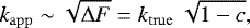
The apparent area and radius ratios ( and kapp, respectively) can be directly estimated from the transit light curve, and are related to the true radius ratio, ktrue, as
 (1)
(1)
where ΔF is the transit depth, and c is the passband-dependent contamination factor. The true radius ratio is derived from kapp then as
 (2)
(2)
The contamination factor depends on the wavelength if the host and contaminant(s) are of different spectral type (i.e. if TEff,H ≠TEff,C), which leads to passband-dependent variations inthe transit depth ( ). Besides the transit depth variations, a subtle colour-dependent signature exists that is directly related to the true radius ratio, and constrains the contamination even if TEff,H = TEff,C (Drake 2003; Tingley 2004; Tingley et al. 2014; Parviainen et al. 2019).
The contamination model yields a contamination estimate for the observed passbands given TEff,H, TEff,C, c, and kapp, where the reference passband for c and kapp is freely chosen (and does not affect the posterior estimate). The contaminated transit model for the passband i is now
 (3)
(3)
where 𝒯 is the uncontaminated transit model.
The final ktrue estimate is marginalised over the contamination allowed by the photometry (and all the other model parameters), including contamination from sources of similar spectral type as the host star 8.
4.3 Log posterior
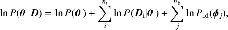
The log posterior for a parameter vector θ given a combined dataset D with nt transits observed in nb unique passbands is
 (4)
(4)
where the first term is the log prior, the second is the total log likelihood, the last term is the sum of the LDTK -calculated log likelihoods for the limb-darkening (when using LDTK to constrain the stellar limb darkening, as explained below), and ϕj is a subset of θ containing the limb darkening coefficients for the jth passband.
4.4 Noise model and log likelihood
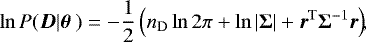
In general, the log likelihood for a single transit light curve assuming normally distributed noise is
 (5)
(5)
where nD is the number of datapoints, r is the residual vector (Fo − F(θ |t, C)), and Σ is the covariance matrix.
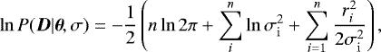
As already mentioned, we experimented using Gaussian processes to model the residual correlated noise not explained by the linear baseline model described below, but chose to simplify our approach after tests against the uncorrelated noise model did not show significant differences. In the end, we chose a normally distributed uncorrelated noise model that leads to the standard likelihood equation,
 (6)
(6)
where σ are the per-point photometric errors. Further, our photometric errors do not show great variations within individual transits, so we chose to use a log-average per-transit photometric error as a free parameter in the model.
Final joint model parametrisation and priors.
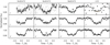 |
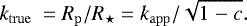
Fig. 3 Three transits of TOI 263.01 observed simultaneously in r′, i′, and zs with MuSCAT2, and three separate transits observed with SINISTRO. Each column shows a separate observing night and each row a separate filter for MuSCAT2 observations, while each column shows a separate transit observed in a separate filter for the LCO data. MuSCAT2 photometry is shown with the original cadences (light grey points) and binned into four-minute bins shown as black points with error bars showing the standard error of the mean. The LCOGT observationsare not binned due to the longer exposure times. The median baseline model has been subtracted from the photometry,and the black lines show the median posterior transit model. |
4.5 Light curve model
The flux for a single observation i is modelled as
 (7)
(7)
where  is the (contaminated) transit model, B is the baseline model, θ is the parameter vector, t is the mid-exposure time, and ci is the covariate vector.
We use the standard quadratic Mandel & Agol transit model (Mandel & Agol 2002) implemented in PYTRANSIT with the triangular parametrisation presented by Kipping (2013).
We use a simple linear model to represent the baseline flux variations as a function of the linear combination of a light-curve-specific set of covariates. The linear model for the final joint analysis was chosen after carrying out analyses for the individual MuSCAT2 and LCO datasets using Gaussian processes (GPs, Rasmussen & Williams 2006; Gibson et al. 2012; Roberts et al. 2013) to model the systematic errors. The GP and linear model analyses agreed with each other, and we chose the computationally faster approach for the final analysis.
4.6 Priors and model parametrisation
4.6.1 Joint model parametrisation
The final joint model needs to reproduce the 47 light curves observed in five passbands with three instruments. This leads to a somewhat complex parametrisation with 160 free parameters, of which between only 5 and 9 are of physical interest.
We divide the model parameters into three main categories. First comes the system parameters that define the orbit and geometry of the planet candidate. These are the quantities that we are most interested in, and are directly connected to the physical properties of the planet candidate. The system parameters do not depend on the observation passband, instrument, or any other external factor, so all the observations contribute to their likelihood. Next comes the passband-dependent parameters such as the stellar limb darkening coefficients and apparent planet-star area ratios. These are quantities that vary as a function of wavelength, and so change from passband to passband, but do not depend on the instrument, observing conditions, and so on. All the observations carried out in a given passband contribute to the likelihoods of the passband-dependent parameters in that passband. Finally, we consider the light-curve-dependent parameters that affect the model of each independent light curve, such as the linear baseline model coefficients. These are unique to each light curve (and instrument) and their posteriors are of little practical interest. However, these parameters need to be included as nuisance parameters to be marginalised over so that their effect on the model is correctly reflected in the uncertainties of the main parameters of interest.
The final parametrisation is outlined in Table 2. The passband-dependent parameters are repeated for each passband, and the light-curve-dependent parameters are repeated for each light curve.
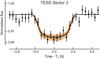 |
Fig. 4 Phase folded and binned TESS Sector 3 light curve (points with uncertainties) and the median transit posterior model with its 16 and 84 percentile limits. The model corresponds to the final joint fit with TESS, MuSCAT2, and LCO observations. The data have been divided by the median baseline model, phase folded, and binned in four-minute bins for visualisation purposes. |
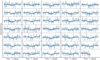 |
Fig. 5 Individual TESS transits with the median posterior transit model and its 68% central posterior limits. |
4.6.2 Baseline coefficients
TESS, LCOGT, and MuSCAT2 all have different sets of covariates for their baseline models. With TESS we include only a constant intercept (the out-of-transit flux level) as a free parameter for each transit. We also carried out analyses with more complex polynomial baseline models and Gaussian processes, but the higher-order polynomial coefficient posteriors agreed with zero, and the GP hyperparameters favoured models dominated by white noise. With MuSCAT2 we include the intercept, median sky level, x- and y-centroid shifts, and aperture entropy (a proxy for FWHM). With LCOGT we include the intercept, airmass, centroid shifts, and FWHM. The intercepts have normal priors centred to unity and standard deviations set to the standard deviation of per-transit flux (σF). The remaining baseline coefficients have normal priors centred around zero with their standard deviations set as for the intercepts.
4.6.3 Stellar limb darkening
Stellar limb darkening is degenerate with the impact parameter and apparent area ratio, and so any assumptions taken about limb darkening can bias the estimates of these two parameters (Csizmadia et al. 2013; Espinoza & Jordan 2015; Parviainen 2018; Parviainen et al. 2019). While multicolour transit photometry can break this degeneracy (limb darkening is passband dependent but the impact parameter and radius ratio are not), we were still interested in understanding how sensitive our analysis results are on our prior assumptions about limb darkening.
For that reason, we repeated all the analyses for two cases. First, we carried out the analyses with a uniform prior on the triangular quadratic limb darkening coefficients from zero to unity (leading to uniform priors covering the physically plausible parameter space of the quadratic coefficients, Kipping 2013). Next, we repeated the analyses using LDTK to constrain the shape of allowed limb darkening profiles (i.e. setting a prior in the limb darkening profile space instead of setting priors on the coefficients themselves, Parviainen & Aigrain 2015).
4.6.4 Contamination
The ground-based photometry has been observed with significantly smaller aperture radii than the TESS photometry, and TESS photometry can a priori be expected to have a different amount of contamination from third light sources than the ground-based photometry. This breaks the prior assumption for the physics-based contamination model described in Sect. 4.2 that the contaminating sources are constant for all the observations. However, the MuSCAT2 and LCOGT photometry was carried out with similar-sized apertures, and the assumption can be considered to hold.
Therefore, we parametrise the model with two contamination factors. The MuSCAT2 and LCOGT transit models use the physics-based contamination model, but the TESS transit model is given an independent unconstrained contamination factor. Further, we do not parametrise the model directly with the true area ratio and contamination, since this was observed to lead to a parameter space that is difficult to sample efficiently with MCMC. We use the apparent and true area ratios instead, where the per-passband contamination levels can be derived using Eqs. (1) and (2).
 |
Fig. 6 Joint and marginal posterior distributions for the key parameters from the modelling of the TESS, MusCAT2, and LCO transitlight curves together. |
5 Results
We show the ground-based photometry with the transit model in Fig. 3, the phase-folded TESS photometry and model in Fig. 4, and the per-transit TESS photometry and model in Fig. 5.
The joint multicolour transit modelling excludes significant levels of blending from sources with effective temperature (TEff,C) different from that of the host star (TEff,H), and also strongly constrains allowed blending from sources with TEff,C ~ TEff,H, as shown in Fig. 6. Grazing transit geometries are also excluded, as the impact parameter is constrained to b < 0.51 at 99% level. The stellar density posterior median of 11 g cm−3 agrees well with theoretical expectations for an M dwarf with TEff ≈ 3200 K.
The median posterior value for the true radius ratio, ktrue, is 0.217, with a 99 posterior percentile value of 0.286. This leads to absolute planetary radius, rp,true, posterior median of 0.87 RJup with a 99 posterior percentile limit of 1.41 RJup. Thus, the candidate radius is in the size range shared both by gas giants and brown dwarfs (Burrows et al. 2011; Chabrier & Baraffe 2000). Unfortunately, uncertainty in rp,true estimate is dominated by the uncertainty in the stellar radius, as illustrated in Fig. 7, and further transit observations would not be able to significantly reduce the uncertainty even if the uncertainty in contamination were brought to zero.
The analysis takes into account the possibility that the transiting object is bright enough to contribute to the total flux significantly.This would be the case of an eclipsing binary system, possibly with close-to identical components. However, our results exclude the possibility that the transiting body would be self-illuminating.
We also carried out a TTV search from the TESS light curves using PyTV (Korth, in prep.), but the S/N ratio of the individual transits was too low for meaningful transit centre estimates.
6 Discussion
TOI 263.01 offers a new puzzle for planetary system formation. If TOI 263.01 is a planet, the lowest-mass possibility would make the object a hot Jupiter with an orbital period of only 0.56 days around a low-mass star. However, such planets have never been observed before. In Fig. 8, we show a period-radius diagram of the currently known transiting planets and brown dwarfs with periods between 0.3 and 200 days and radii between 0 and 2 RJup, with the position of TOI 263.01 marked with a star. TOI 263.01 lies in a thus-far unexplored parameter space. Further, if we remove all spectral hosts with TEff > 4000 K, TOI 263 becomes unique and isolated. It is possible we are capturing the initial stages of a compact ultra-short-period planet formation, before the planet can lose its atmosphere.
Given the uncertainty in the determination of the radius of TOI 263.01, and the degeneracy of the mass–radius relationship for planets and brown dwarfs more massive than 0.5 MJup (eg. Baraffe et al. 2003), there is a non-negligible probability that our target is a high-mass planet or a brown dwarf with a mass in the interval 13 MJup < M < 75 MJup . This would make TOI 263 an even more exciting system, representing a unique and extreme case in the (disputed) “brown dwarf desert” (Marcy & Butler 2000, but see also Carmichael et al. 2019 and Persson et al. 2019), with the period of the transiting body falling between the 10.6 h orbital period of CVSO 30b (van Eyken et al. 2012, labelled in Fig. 8) and the 16.2 h orbital period of the recently discovered NGTS-7Ab (Jackman et al. 2019, labelled in Fig. 8). Given the evidence that CSVO-30b is likely not a planet (Yu et al. 2015; Lee 2017), TOI 263.01 and NGTS-7Ab are the only currently known short-period massive objects of their kind orbiting M dwarfs.
In general, only a handful of massive transiting planets and brown dwarfs are known to orbit around M-dwarf host stars, and all except NGTS-7Ab have orbital periods greater than one day, as shown in Fig. 8. These planets are (1) Kepler-45b (Johnson et al. 2012), (2) NGTS-1b (Bayliss et al. 2018), (3) HATS-6b (Hartman et al. 2015), (4) HATS-71Ab (Bakos et al. 2018), and (5) GJ 674b (Bonfils et al. 2007); and the brown dwarfs are (I) LP 261-75b (Reid & Walkowicz 2006), (II) AD 3116b (Gillen et al. 2017), and (III) NLTT 41135b (Irwin et al. 2010); this is excluding objects with periods larger than 200 days and radii larger than 2 RJup, although the recent discovery of GJ 3512 (Morales et al. 2019) with an orbital period of 204 days deserves to be mentioned. At the moment these objects or their host stars do not seem to share any clear common characteristics. NLTT 41135b and HATS-71b orbit a host in a binary system (HATS-71b likely), AD 3116 is a member of the Praesepe cluster, while HATS-6b would seem to be very normal warm Saturn orbiting a normal M1 star.
The existence of a massive planet or a brown dwarf at an orbital period of 0.56 d around an M3.5 dwarf star is very hard to explain using formation models based on core-accretion processes given the high migration rate of planet seeds around these low-mass stars (Johansen et al. 2019). These companions may be explained by disc fragmentation mechanisms at large separations from the parent star and later migration to close-in orbits (Morales et al. 2019). However, this model is yet to be proven and TOI 263.01 would become an excellent target for this endeavour before the massive planet or brown dwarf becomes engulfed by its parent star as predicted by the disc-fragmentation model (Armitage & Bonnell 2002).
TOI 263 is indeed a rare system among the thousands of transiting objects discovered to date because it offers an exclusive opportunity to constrain the formation models of the birth of planets and brown dwarfs. The next step for this system is to determine the mass of TOI 263.01 using RV measurements. While TOI 263 is very faint, such measurements may be possible due to the low mass of the host star. At the low-mass end (Mp ≈ 0.5 MJup ), we can expect an RV semi-amplitude of 250 m s−1, while at the high-mass end (Mp ≈ 75 MJup ) it could be around 35 km s−1.
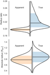 |
Fig. 7 Apparent and true radius ratio posteriors (above), and apparent and true candidate radius posteriors (below). Allowing for blending creates a tail towards high radius ratios, in this case corresponding to possible blending with TEff,H ~ TEff,C, but this hasonly a minor effect on the absolute planet radius posterior, which is dominated by the uncertainty in the stellar radius. |
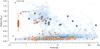 |
Fig. 8 Period–radius diagram of the confirmed transiting extrasolar planets (exoplanet.eu, Schneider et al. 2011, accessed 4.5.2019) and brown dwarfs (collected from Carmichael et al. 2019; Persson et al. 2019; Jackman et al. 2019) to date with periods between 0.3 and 200 days and radii between 0 and 2 RJup. TOI 263.01 is marked with a black-edged white star with 68 and 99% central posterior intervals for its true radius marked with dark and light orange shading, respectively. Planets around host stars with TEff < 4000 K are marked with orange-edged stars, and the distribution of planets around hotter stars is shown with blue shading. Brown dwarfs around host stars with TEff < 4000 K are marked with orange-edged circles, and the brown dwarfs around hotter hosts are marked with dark-blue-edged circles. The numbered planets and brown dwarfs are described in Sect. 6. |
Relative and absolute estimates for the stellar and planetary parameters derived from the multicolour transit analysis.
Acknowledgements
First, we thank the anonymous referee for their helpful and constructive comments. We acknowledge financial support from the Agencia Estatal de Investigación of the Ministerio de Ciencia, Innovación y Universidades and the European FEDER/ERF funds through projects ESP2013-48391-C4-2-R, AYA2016-79425-C3-2-P, AYA2015-69350-C3-2-P. This work is partly financed by the Spanish Ministry of Economics and Competitiveness through project ESP2016-80435-C2-2-R. N.N. acknowledges supports by JSPS KAKENHI Grant Numbers JP18H01265 and JP18H05439, and JST PRESTO Grant Number JPMJPR1775. J.K. acknowledges support by Deutsche Forschungsgemeinschaft (DFG) grants PA525/18-1 and PA525/19-1 within the DFG Schwerpunkt SPP 1992, Exploring the Diversity of Extra-solar Planets. This article is partly based on observations made with the MuSCAT2 instrument, developed by ABC, at Telescopio Carlos Sánchez operated on the island of Tenerife by the IAC in the Spanish Observatorio del Teide. We acknowledge the use of public TESS Alert data from pipelines at the TESS Science Office and at the TESS Science Processing Operations Center. This work makes use of observations from the LCOGT network. Resources supporting this work were provided by the NASA High-End Computing (HEC) Program through the NASA Advanced Supercomputing (NAS) Division at Ames Research Center for the production of the SPOC data products. This work makes use of observations from the LCOGT network.
References
- Almenara, J. M., Deeg, H. J., Aigrain, S., et al. 2009, A&A, 506, 337 [NASA ADS] [CrossRef] [EDP Sciences] [Google Scholar]
- Alonso-Floriano, F. J., Morales, J. C., Caballero, J. A., et al. 2015, A&A, 577, A128 [NASA ADS] [CrossRef] [EDP Sciences] [Google Scholar]
- Armitage, P. J., & Bonnell, I. A. 2002, MNRAS, 330, L11 [NASA ADS] [CrossRef] [Google Scholar]
- Astropy Collaboration (Robitaille, T. P., et al.) 2013, A&A, 558, A33 [NASA ADS] [CrossRef] [EDP Sciences] [Google Scholar]
- Bakos, G. Á., Bayliss, D., Bento, J., et al. 2018, AJ, submitted [arXiv:1812.09406] [Google Scholar]
- Baraffe, I., Chabrier, G., Barman, T. S., Allard, F., & Hauschildt, P. H. 2003, A&A, 402, 701 [NASA ADS] [CrossRef] [EDP Sciences] [Google Scholar]
- Bayliss, D., Gillen, E., Eigmüller, P., et al. 2018, MNRAS, 475, 4467 [NASA ADS] [CrossRef] [Google Scholar]
- Bonfils, X., Mayor, M., Delfosse, X., et al. 2007, A&A, 474, 293 [NASA ADS] [CrossRef] [EDP Sciences] [Google Scholar]
- Bradley, L., Sipocz, B., Robitaille, T., et al. 2019, https://doi.org/10.5281/zenodo.1292315 [Google Scholar]
- Brown, T. M., Baliber, N., Bianco, F. B., et al. 2013, PASP, 125, 1031 [NASA ADS] [CrossRef] [Google Scholar]
- Burrows, A. S., Heng, K., & Nampaisarn, T. 2011, ApJ, 736, 47 [NASA ADS] [CrossRef] [Google Scholar]
- Cabrera, J., Barros, S. C. C., Armstrong, D., et al. 2017, A&A, 606, A75 [NASA ADS] [CrossRef] [EDP Sciences] [Google Scholar]
- Cameron, A. C. 2012, Nature, 492, 48 [NASA ADS] [CrossRef] [Google Scholar]
- Carmichael, T. W., Latham, D. W., & Vanderburg, A. M. 2019, AJ, 158, 38 [NASA ADS] [CrossRef] [Google Scholar]
- Chabrier, G., & Baraffe, I. 2000, ARA&A, 38, 337 [NASA ADS] [CrossRef] [Google Scholar]
- Collins, K. A., Kielkopf, J. F., Stassun, K. G., & Hessman, F. V. 2017, AJ, 153, 77 [NASA ADS] [CrossRef] [Google Scholar]
- Csizmadia, S., Pasternacki, T., Dreyer, C., et al. 2013, A&A, 549, A9 [NASA ADS] [CrossRef] [EDP Sciences] [Google Scholar]
- Drake, A. J. 2003, ApJ, 589, 1020 [NASA ADS] [CrossRef] [Google Scholar]
- Espinoza, N., & Jordan, A. 2015, MNRAS, 450, 1879 [NASA ADS] [CrossRef] [Google Scholar]
- Foreman-Mackey, D., Hogg, D. W., Lang, D., & Goodman, J. 2013, PASP, 125, 306 [CrossRef] [Google Scholar]
- Fressin, F., Torres, G., Charbonneau, D., et al. 2013, ApJ, 766, 81 [NASA ADS] [CrossRef] [Google Scholar]
- Gibson, N. P., Aigrain, S., Roberts, S., et al. 2012, MNRAS, 419, 2683 [NASA ADS] [CrossRef] [Google Scholar]
- Gillen, E., Hillenbrand, L. A., David, T. J., et al. 2017, ApJ, 849, 11 [NASA ADS] [CrossRef] [Google Scholar]
- Goodman, J., & Weare, J. 2010, Commun. Appl. Math. Comput. Sci., 5, 65 [Google Scholar]
- Hartman, J. D., Bayliss, D., Brahm, R., et al. 2015, AJ, 149, 166 [NASA ADS] [CrossRef] [Google Scholar]
- Hoyer, S., & Hamman, J. J. 2017, J. Open Res. Softw., 5, 1 [CrossRef] [Google Scholar]
- Hunter, J. D. 2007, Comput. Sci. Eng., 9, 90 [NASA ADS] [CrossRef] [Google Scholar]
- Husser, T.-O., Wende-von Berg, S., Dreizler, S., et al. 2013, A&A, 553, A6 [NASA ADS] [CrossRef] [EDP Sciences] [Google Scholar]
- Irwin, J., Buchhave, L., Berta, Z. K., et al. 2010, ApJ, 718, 1353 [NASA ADS] [CrossRef] [Google Scholar]
- Jackman, J. A. G., Wheatley, P. J., Bayliss, D., et al. 2019, MNRAS, 489, 5146 [NASA ADS] [CrossRef] [Google Scholar]
- Jenkins, J. M., Twicken, J. D., McCauliff, S., et al. 2016, Proc. SPIE, 9913, 99133E [Google Scholar]
- Jensen, E. 2013, Astrophysics Source Code Library [record ascl:1306.007] [Google Scholar]
- Johansen, A., Ida, S., & Brasser, R. 2019, A&A, 622, A202 [NASA ADS] [CrossRef] [EDP Sciences] [Google Scholar]
- Johnson, J. A., Gazak, J. Z., Apps, K., et al. 2012, AJ, 143, 5 [Google Scholar]
- Kipping, D. M. 2013, MNRAS, 435, 2152 [Google Scholar]
- Kirkpatrick, J. D., Schneider, A., Fajardo-Acosta, S., et al. 2014, ApJ, 783, 2 [NASA ADS] [CrossRef] [Google Scholar]
- Lang, D., Hogg, D. W., Mierle, K., Blanton, M., & Roweis, S. 2010, AJ, 139, 1782 [Google Scholar]
- Lee, C.-H. 2017, Res. Notes AAS, 1, 41 [NASA ADS] [CrossRef] [Google Scholar]
- Maldonado, J., Affer, L., Micela, G., et al. 2015, A&A, 577, A132 [NASA ADS] [CrossRef] [EDP Sciences] [Google Scholar]
- Mandel, K., & Agol, E. 2002, ApJ, 580, L171 [NASA ADS] [CrossRef] [Google Scholar]
- Marcy, G. W., & Butler, R. P. 2000, PASP, 112, 137 [NASA ADS] [CrossRef] [Google Scholar]
- Martin, E., Rebolo, R., & Zapatero-Osorio, M. 1996, ApJ, 469, 706 [NASA ADS] [CrossRef] [Google Scholar]
- Mckinney, W. 2010, Data structures for statistical computing in Python, in 9th Python in Science Conference, 1697900, 51 [Google Scholar]
- Morales, J. C., Mustill, A. J., Ribas, I., et al. 2019, Science, 365, 1441 [NASA ADS] [CrossRef] [Google Scholar]
- Moutou, C., Pont, F., Bouchy, F., et al. 2009, A&A, 506, 321 [NASA ADS] [CrossRef] [EDP Sciences] [Google Scholar]
- Mullally, F., Thompson, S. E., Coughlin, J. L., Burke, C. J., & Rowe, J. F. 2018, AJ, 155, 210 [NASA ADS] [CrossRef] [Google Scholar]
- Narita, N., Fukui, A., Kusakabe, N., et al. 2019, J. Astron. Telesc. Instrum. Syst., 5, 015001 [NASA ADS] [Google Scholar]
- Navascus, D. B. y., & Martín, E. L. 2003, AJ, 126, 2997 [NASA ADS] [CrossRef] [Google Scholar]
- Parviainen, H. 2015, MNRAS, 450, 3233 [NASA ADS] [CrossRef] [Google Scholar]
- Parviainen, H. 2018, in Handbook of Exoplanet (Cham: Springer International Publishing), 1 [Google Scholar]
- Parviainen, H., & Aigrain, S. 2015, MNRAS, 453, 3822 [NASA ADS] [CrossRef] [Google Scholar]
- Parviainen, H., Tingley, B., Deeg, H. J., et al. 2019, A&A, 630, A89 [NASA ADS] [CrossRef] [EDP Sciences] [Google Scholar]
- Pecaut, M. J.,& Mamajek, E. E. 2013, ApJS, 208, 9 [NASA ADS] [CrossRef] [Google Scholar]
- Perez, F., & Granger, B. 2007, Comput. Sci. Eng., 21 [Google Scholar]
- Persson, C. M., Csizmadia, S., Mustill, A. J., et al. 2019, A&A, 628, A64 [NASA ADS] [CrossRef] [EDP Sciences] [Google Scholar]
- Price, K., Storn, R., & Lampinen, J. 2005, Differential Evolution (Berlin: Springer) [Google Scholar]
- Rajpurohit, A. S., Reylé, C., Allard, F., et al. 2013, A&A, 556, A15 [NASA ADS] [CrossRef] [EDP Sciences] [Google Scholar]
- Rasmussen, C. E., & Williams, C. 2006, Gaussian Processes for Machine Learning (Cambridge: The MIT Press) [Google Scholar]
- Reid, I. N., & Walkowicz, L. M. 2006, PASP, 118, 671 [NASA ADS] [CrossRef] [Google Scholar]
- Roberts, S., Osborne, M., Ebden, M., et al. 2013, Philos. Trans. A. Math. Phys. Eng. Sci., 371, 20110550 [NASA ADS] [Google Scholar]
- Rosenblatt, F. 1971, Icarus, 14, 71 [NASA ADS] [CrossRef] [Google Scholar]
- Santerne, A., Díaz, R. F., Moutou, C., et al. 2012, A&A, 545, A76 [NASA ADS] [CrossRef] [EDP Sciences] [Google Scholar]
- Schlieder, J. E., Lépine, S., Rice, E., et al. 2012, AJ, 143, 114 [NASA ADS] [CrossRef] [Google Scholar]
- Schneider, J., Dedieu, C., Le Sidaner, P., Savalle, R., & Zolotukhin, I. 2011, A&A, 532, A79 [NASA ADS] [CrossRef] [EDP Sciences] [Google Scholar]
- Schweitzer, A., Passegger, V. M., Cifuentes, C., et al. 2019, A&A, 625, A68 [NASA ADS] [CrossRef] [EDP Sciences] [Google Scholar]
- Storn, R., & Price, K. 1997, J. Glob. Optim., 11, 341 [Google Scholar]
- Tingley, B. 2004, A&A, 425, 1125 [NASA ADS] [CrossRef] [EDP Sciences] [Google Scholar]
- Tingley, B., Parviainen, H., Gandolfi, D., et al. 2014, A&A, 567, A14 [NASA ADS] [CrossRef] [EDP Sciences] [Google Scholar]
- Twicken, J. D., Catanzarite, J. H., Clarke, B. D., et al. 2018, PASP, 130, 064502 [NASA ADS] [CrossRef] [Google Scholar]
- van der Walt, S., Colbert, S. C., & Varoquaux, G. 2011, Comput. Sci. Eng., 13, 22 [Google Scholar]
- van Eyken, J. C., Ciardi, D. R., von Braun, K., et al. 2012, ApJ, 755, 42 [NASA ADS] [CrossRef] [Google Scholar]
- Yu, L., Winn, J. N., Gillon, M., et al. 2015, ApJ, 812, 48 [NASA ADS] [CrossRef] [Google Scholar]
Considering the existing instruments, RV follow-up could be feasible using the 4-VLT mode of ESPRESSO.
The effects from a self-illuminating transiting body contributing flux to the light curve are the same as from a contaminating third body, and are modelled by the approach without any special modifications.
Image Reduction and Analysis Facility (IRAF) is distributed by the National Optical Astronomy Observatories, which are operated by the Association of Universities for Research in Astronomy, Inc., under contract with the National Science Foundation.
The analysis is valid also in the case of a self-illuminating transiting object, such as in the case of an eclipsing binary system.
All Tables
Relative and absolute estimates for the stellar and planetary parameters derived from the multicolour transit analysis.
All Figures
|
Fig. 1 MuSCAT2 field observed in i′ band with TOI 263 marked with a “0” and the rest of the stars numbered from brightest to faintest. The circles show the apertures used to extract the photometry, and the two outermost circles mark the annulus used to measure the sky level. The dotted circle marks a 2′ circle centred around TOI 263. |
| In the text | |
|
Fig. 2 ALFOSC spectrum of TOI 263 with a resolution of 16.6 Å is plotted as a red line. It is compared to the spectra of three spectral standard stars from the catalogue of Alonso-Floriano et al. (2015), which are shown with a black line: GJ 2066 (J08161+013, M2V), Luyten’s star (J07274+052, M3.5V), and V1352 Ori (J05421+124, M4V). All spectra are normalised to 1.0 at the red continuum of the subordinate Na I lines, and are shifted vertically by 1.0 for clarity. The strongest molecular and atomic features are indicated on the top. The strongest telluric oxygen features are also labelled. |
| In the text | |
|
Fig. 3 Three transits of TOI 263.01 observed simultaneously in r′, i′, and zs with MuSCAT2, and three separate transits observed with SINISTRO. Each column shows a separate observing night and each row a separate filter for MuSCAT2 observations, while each column shows a separate transit observed in a separate filter for the LCO data. MuSCAT2 photometry is shown with the original cadences (light grey points) and binned into four-minute bins shown as black points with error bars showing the standard error of the mean. The LCOGT observationsare not binned due to the longer exposure times. The median baseline model has been subtracted from the photometry,and the black lines show the median posterior transit model. |
| In the text | |
|
Fig. 4 Phase folded and binned TESS Sector 3 light curve (points with uncertainties) and the median transit posterior model with its 16 and 84 percentile limits. The model corresponds to the final joint fit with TESS, MuSCAT2, and LCO observations. The data have been divided by the median baseline model, phase folded, and binned in four-minute bins for visualisation purposes. |
| In the text | |
|
Fig. 5 Individual TESS transits with the median posterior transit model and its 68% central posterior limits. |
| In the text | |
|
Fig. 6 Joint and marginal posterior distributions for the key parameters from the modelling of the TESS, MusCAT2, and LCO transitlight curves together. |
| In the text | |
|
Fig. 7 Apparent and true radius ratio posteriors (above), and apparent and true candidate radius posteriors (below). Allowing for blending creates a tail towards high radius ratios, in this case corresponding to possible blending with TEff,H ~ TEff,C, but this hasonly a minor effect on the absolute planet radius posterior, which is dominated by the uncertainty in the stellar radius. |
| In the text | |
|
Fig. 8 Period–radius diagram of the confirmed transiting extrasolar planets (exoplanet.eu, Schneider et al. 2011, accessed 4.5.2019) and brown dwarfs (collected from Carmichael et al. 2019; Persson et al. 2019; Jackman et al. 2019) to date with periods between 0.3 and 200 days and radii between 0 and 2 RJup. TOI 263.01 is marked with a black-edged white star with 68 and 99% central posterior intervals for its true radius marked with dark and light orange shading, respectively. Planets around host stars with TEff < 4000 K are marked with orange-edged stars, and the distribution of planets around hotter stars is shown with blue shading. Brown dwarfs around host stars with TEff < 4000 K are marked with orange-edged circles, and the brown dwarfs around hotter hosts are marked with dark-blue-edged circles. The numbered planets and brown dwarfs are described in Sect. 6. |
| In the text | |
Current usage metrics show cumulative count of Article Views (full-text article views including HTML views, PDF and ePub downloads, according to the available data) and Abstracts Views on Vision4Press platform.
Data correspond to usage on the plateform after 2015. The current usage metrics is available 48-96 hours after online publication and is updated daily on week days.
Initial download of the metrics may take a while.