| Issue |
A&A
Volume 633, January 2020
|
|
|---|---|---|
| Article Number | A64 | |
| Number of page(s) | 26 | |
| Section | Astronomical instrumentation | |
| DOI | https://doi.org/10.1051/0004-6361/201834996 | |
| Published online | 14 January 2020 | |
Polarimetric imaging mode of VLT/SPHERE/IRDIS
II. Characterization and correction of instrumental polarization effects⋆,⋆⋆
1
Leiden Observatory, Leiden University, PO Box 9513, 2300 RA Leiden, The Netherlands
e-mail: This email address is being protected from spambots. You need JavaScript enabled to view it.
2
European Southern Observatory, Alonso de Córdova 3107, Casilla, 19001 Vitacura, Santiago, Chile
3
Space Telescope Science Institute, Baltimore 21218 MD, USA
4
Université Grenoble Alpes, CNRS, IPAG, 38000 Grenoble, France
5
Faculty of Aerospace Engineering, Delft University of Technology, Kluyverweg 1, 2629 HS Delft, The Netherlands
6
Anton Pannekoek Institute for Astronomy, University of Amsterdam, Science Park 904, 1098 XH Amsterdam, The Netherlands
7
ETH Zurich, Institute for Particle Physics and Astrophysics, Wolfgang-Pauli-Strasse 27, 8093 Zurich, Switzerland
8
CRAL, UMR 5574, CNRS, Université de Lyon, Ecole Normale Supérieure de Lyon, 46 allée d’Italie, 69364 Lyon Cedex 07, France
9
Aix Marseille Univ, CNRS, CNES, LAM, Marseille, France
10
Max Planck Institute for Astronomy, Königstuhl 17, 69117 Heidelberg, Germany
11
Heidelberg University, Institute of Theoretical Astrophysics, Albert-Ueberle-Str. 2, 69120 Heidelberg, Germany
12
Université Côte d’Azur, OCA, CNRS, Lagrange, France
13
INAF – Osservatorio Astronomico di Padova, Vicolo della Osservatorio 5, 35122 Padova, Italy
14
DOTA, ONERA, Université Paris Saclay, 91123 Palaiseau, France
15
LESIA, Observatoire de Paris, PSL Research University, CNRS, Sorbonne Universités, UPMC, Univ. Paris 06, Univ. Paris Diderot, Sorbonne Paris Cité, 5 place Jules Janssen, 92195 Meudon, France
16
Geneva Observatory, University of Geneva, Chemin des Mailettes 51, 1290 Versoix, Switzerland
Received:
29
December
2018
Accepted:
14
October
2019
Abstract
Context. Circumstellar disks and self-luminous giant exoplanets or companion brown dwarfs can be characterized through direct-imaging polarimetry at near-infrared wavelengths. SPHERE/IRDIS at the Very Large Telescope has the capabilities to perform such measurements, but uncalibrated instrumental polarization effects limit the attainable polarimetric accuracy.
Aims. We aim to characterize and correct the instrumental polarization effects of the complete optical system, that is, the telescope and SPHERE/IRDIS.
Methods. We created a detailed Mueller matrix model in the broadband filters Y, J, H, and Ks and calibrated the model using measurements with SPHERE’s internal light source and observations of two unpolarized stars. We developed a data-reduction method that uses the model to correct for the instrumental polarization effects, and applied it to observations of the circumstellar disk of T Cha.
Results. The instrumental polarization is almost exclusively produced by the telescope and SPHERE’s first mirror and varies with telescope altitude angle. The crosstalk primarily originates from the image derotator (K-mirror). At some orientations, the derotator causes severe loss of signal (> 90% loss in the H- and Ks-band) and strongly offsets the angle of linear polarization. With our correction method we reach, in all filters, a total polarimetric accuracy of ≲0.1% in the degree of linear polarization and an accuracy of a few degrees in angle of linear polarization.
Conclusions. The correction method enables us to accurately measure the polarized intensity and angle of linear polarization of circumstellar disks, and is a vital tool for detecting spatially unresolved (inner) disks and measuring the polarization of substellar companions. We have incorporated the correction method in a highly-automated end-to-end data-reduction pipeline called IRDAP, which we made publicly available online.
Key words: polarization / techniques: polarimetric / techniques: high angular resolution / techniques: image processing / methods: observational / protoplanetary disks
Based on observations made with ESO telescopes at the La Silla Paranal Observatory under program ID 60.A-9800(S), 60.A-9801(S) and 096.C-0248(C).
The data-reduction pipeline IRDAP is available at https://irdap.readthedocs.io
© ESO 2020
1. Introduction
The near-infrared (NIR) polarimetric mode of the high-contrast imager SPHERE/IRDIS at the Very Large Telescope (VLT), which we introduced in Paper I (de Boer et al. 2020), has proven to be very successful for the detection of circumstellar disks in scattered light (Garufi et al. 2017) and shows much promise for the characterization of exoplanets and companion brown dwarfs (see van Holstein et al. 2017). However, studies of circumstellar disks are often limited to analyses of the orientation (position angle and inclination) and morphology (rings, gaps, cavities, and spiral arms) of the disks (e.g., Muto et al. 2012; Quanz et al. 2013; Ginski et al. 2016; de Boer et al. 2016). Quantitative polarimetric measurements of circumstellar disks and substellar companions are currently very challenging because existing data-reduction methods do not account for instrumental polarization effects with a sufficiently high accuracy.
Due to instrumental polarization effects, polarized signal arriving at IRDIS’ detector is different from that incident on the telescope. The two predominant effects are instrumental polarization (IP), that is, polarization signals produced by the instrument or telescope, and crosstalk, that is, instrument- or telescope-induced mixing of polarization states. IP not only changes the polarization state of an object, but can also make unpolarized sources appear polarized if not accounted for. For astronomical targets with a relatively low degree of linear polarization, IP can induce a significant rotation of the angle of linear polarization. Crosstalk also causes an offset of the measured angle of linear polarization and can lower the polarimetric efficiency, that is, the fraction of the incident or true linear polarization that is actually measured. We first encountered these instrumental polarization effects when observing the disk around TW Hydrae as described in Paper I.
To derive the true polarization state of the light incident on the telescope, we need to calibrate the instrument so that we know the instrumental polarization effects a priori. This enables us to accurately and quantitatively measure the polarization of circumstellar disks and substellar companions. In addition, it enables accurate mapping of extended objects other than circumstellar disks, such as solar system objects, molecular clouds, and galaxies (e.g., Gratadour et al. 2015), provided the target is sufficiently bright for the adaptive optics correction.
For observations of circumstellar disks (see Paper I), calibrating the instrument yields a multitude of improvements. Firstly, the calibration allows for more accurate studies of the orientation and morphology of the disks, especially at the innermost regions (separation < 0.5″). In fact, we are able to deduce the presence of spatially unresolved (inner) disks by measuring the polarization signals of the stars (see e.g., Keppler et al. 2018). Secondly, the calibration enables more accurate measurements of the angle of linear polarization. This in turn allows us to prove the presence of non-azimuthal polarization (Canovas et al. 2015) that can be indicative of multiple scattering or the presence of a binary star, and allows for a more in-depth study of dust properties. Finally, the calibration enables more accurate measurements of the polarized intensity, that is, the polarized surface brightness of the disk.
More accurate measurements of the polarized surface brightness enables us to construct scattering phase functions (e.g., Perrin et al. 2015; Stolker et al. 2016; Ginski et al. 2016; Milli et al. 2017), perform more accurate radiative transfer modeling (e.g., Pinte et al. 2009; Min et al. 2009; Pohl et al. 2017a; Keppler et al. 2018), and determine dust particle properties (e.g., Min et al. 2012; Pohl et al. 2017a,b). In addition, it allows for accurate measurements of the degree of linear polarization of the disk, enabling us to further constrain dust properties (e.g., Perrin et al. 2009, 2015; Milli et al. 2015). However, before images of the degree of linear polarization can be constructed, an image of the total intensity of the disk needs to be obtained, for example with reference star differential imaging (RDI; e.g., Canovas et al. 2013) or, for disks viewed edge-on, with angular differential imaging (ADI; Marois et al. 2006).
To measure polarization signals of young self-luminous giant exoplanets or companion brown dwarfs (see Paper I), it is of vital importance to calibrate the instrument. Based on radiative transfer models, the NIR degree of linear polarization of a companion can be a few tenths of a percent up to several percent (de Kok et al. 2011; Marley & Sengupta 2011; Stolker et al. 2017). Measurements of these small polarization signals therefore need to be performed with a very high accuracy, which is only possible after careful calibration of the instrumental polarization effects.
Polarimetric measurements of substellar companions have already been attempted by Millar-Blanchaer et al. (2015) and Jensen-Clem et al. (2016) with the Gemini Planet Imager (GPI), and by van Holstein et al. (2017) with SPHERE/IRDIS (using the calibration results presented in this paper). No polarization signals were detected in these studies. Recently, Ginski et al. (2018) presented the first direct detection of a polarization signal from a substellar companion. Using the calibration results presented in this paper, they find the companion to CS Cha to have a NIR degree of linear polarization of 14%, which suggests the presence of a spatially unresolved disk and dusty envelope around the companion.
In this paper, we characterize the instrumental polarization effects of the complete optical system of VLT/SPHERE/IRDIS, that is, the telescope and the instrument, in the four broadband filters Y, J, H, and Ks. Because the complexity of the optical path is comparable to that of solar telescopes and their instruments, we perform a calibration similar to those applied in the field of solar physics (see e.g., Skumanich et al. 1997; Beck et al. 2005; Socas-Navarro et al. 2011). For our calibration, we create a detailed Mueller matrix model of the optical path and determine the parameters of the model from measurements with SPHERE’s internal light source and observations of two unpolarized stars. Similar approaches have been adopted for the German Vacuum Tower Telescope (Beck et al. 2005), VLT/NACO (Witzel et al. 2011) and GPI (Wiktorowicz et al. 2014; Millar-Blanchaer et al. 2016). We then develop a data-reduction method to correct science measurements for the instrumental polarization effects using the model, and exemplify this correction method and its advantages with polarimetric observations of the circumstellar disk of T Cha from Pohl et al. (2017a). This work is Paper II of a larger study in which Paper I discusses IRDIS’ polarimetric mode, the data reduction, and recommendations for observations and instrument upgrades.
With our instrument model we aim to achieve in all four broadband filters a total polarimetric accuracy, that is, the uncertainty in the measured polarization signal, of ∼0.1% in the degree of linear polarization. In addition, we aim to attain an accuracy of a few degrees in angle of linear polarization in these filters. Reaching these accuracies enables us to measure the linear polarization of substellar companions (we regard the extremely high degree of linear polarization found by Ginski et al. 2018 to be an exception). These accuracies also readily suffice for quantitative polarimetry of circumstellar disks, because the degree of linear polarization of disks is typically much higher than that of substellar companions: on the order of percents to several ten percent (see e.g., Perrin et al. 2009). To attain a total polarimetric accuracy of ∼0.1%, an absolute polarimetric accuracy, that is, the uncertainty in the instrumental polarization (IP), of ≤0.1% and a relative polarimetric accuracy, that is, the uncertainty that scales with the input polarization signal, of < 1% is aimed for.
The outline of this paper is as follows. In Sect. 2 we present the conventions and definitions used throughout this paper. Subsequently, we briefly review the SPHERE/IRDIS optical path and discuss the expected instrumental polarization effects in Sect. 3. We explain the Mueller matrix model describing these effects in Sect. 4. In Sects. 5 and 6 we determine the parameters of the model from measurements with the internal light source and observations of two unpolarized stars, respectively. We then discuss the accuracy of the model in Sect. 7. In Sect. 8 we present our correction method and exemplify it with polarimetric observations of the circumstellar disk of T Cha. In the same section we describe the improvements we attain with respect to conventional data-reduction methods, discuss the limits to and optimization of the polarimetric accuracy, and introduce our data-reduction pipeline that incorporates the correction method. Finally, we present conclusions in Sect. 9. If the reader is only interested in applying our correction method to on-sky data, one could suffice with reading Sects. 2, 3, 8 and 9.
2. Conventions and definitions
In this section we briefly outline the conventions and definitions used throughout this paper. The total intensity and polarization state of a beam of light can be described by a Stokes vector S (e.g., Tinbergen 2005):
 (1)
(1)
where I is the total intensity (or flux), Q and U describe linear polarization and V represents circular polarization. We define these Stokes parameters with respect to the general reference frame shown in Fig. 1. Positive Stokes Q (+Q) and negative Stokes Q (−Q) correspond to vertical and horizontal linear polarization, respectively. When looking into the beam of light, positive (negative) Stokes U is oriented 45° counterclockwise (clockwise) from positive Stokes Q. Finally, positive (negative) Stokes V is defined as circularly polarized light with clockwise (counterclockwise) rotation when looking into the beam of light.
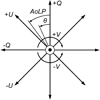 |
Fig. 1. Reference frame for the definition of the Stokes parameters describing the oscillation direction of the electric field within a beam of light. The propagation direction of the light beam is out of the paper, toward the reader. Positive and negative Stokes Q are oriented along the vertical (+Q) and horizontal (−Q) axes, respectively. Looking into the beam of light, positive Stokes U (+U) is oriented 45° counterclockwise from positive Stokes Q and positive Stokes V (+V) is defined as clockwise rotation. The angle of linear polarization AoLP and the rotation angle θ of an optical component used in the rotation Mueller matrix (see Eqs. (15) and (16)) are defined counterclockwise when looking into the beam of light. |
We can normalize the Stokes vector of Eq. (1) by dividing each of its Stokes parameters by the total intensity I:
![Mathematical equation: $$ \begin{aligned} \boldsymbol{S} = \left[1,\,q,\,u,\,v\right]^\mathrm{T} , \end{aligned} $$](/articles/aa/full_html/2020/01/aa34996-18/aa34996-18-eq2.gif) (2)
(2)
with q, u, and v the normalized Stokes parameters. From the Stokes parameters we can calculate the linearly polarized intensity (PIL), degree of linear polarization (DoLP) and angle of linear polarization (AoLP; see Fig. 1) as follows:
 (3)
(3)
 (4)
(4)
 (5)
(5)
3. Optical path and instrumental polarization effects of SPHERE/IRDIS
3.1. SPHERE/IRDIS optical path
Before discussing the instrumental polarization effects expected for SPHERE/IRDIS, in this section we first summarize the optical path and the working principle of IRDIS’ polarimetric mode. As described in detail in Paper I, SPHERE’s optical system is complex and has many rotating components. A simplified version of the optical path is shown in Fig. 2. The model parameters, Stokes vectors and the top right part of the image are discussed in Sect. 4.
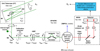 |
Fig. 2. Overview of the optical path of the complete optical system, i.e., the Unit Telescope (UT) and SPHERE/IRDIS, showing only the components relevant for polarimetric measurements (image adapted from Fig. 2 of Paper I). The names of the (groups of) components are indicated in boldface. The black circular arrows indicate the astronomical target’s parallactic angle p, the telescope’s rotation with the altitude angle a, the offset angle of the calibration polarizer δcal, and the rotation of the HWP and image derotator with the angles θHWP + δHWP and θder + δder, respectively. Also shown are the parameters describing the instrumental polarization effects of the (groups of) components: the component diattenuations ϵ, retardances 𝛥 and the polarizer diattenuation d. The Stokes vectors Sin, SHWP, Sdet, L, Sdet, R and |

During an observation, light is collected by the altazimuth-mounted Unit Telescope (UT) which consists of three mirrors. The incident light hits the primary mirror (M1) and is subsequently re-focused by the secondary mirror (M2) that is suspended at the top of the telescope tube. The flat tertiary mirror (M3) has an angle of incidence of 45° and reflects the beam of light to the Nasmyth platform where SPHERE is located. When the telescope tracks a target across the sky, the target rotates with the parallactic angle in the pupil of the UT and the UT rotates with the telescope altitude angle with respect to Nasmyth platform.
The light entering SPHERE (Beuzit et al. 2019) passes a system that can feed the instrument with light from an internal light source to enable internal calibrations (Wildi et al. 2009; Roelfsema et al. 2010). Subsequently, the beam of light hits the flat mirror M4 (the pupil tip-tilt mirror) that similarly to M3 is coated with aluminum and has a 45° inclination angle. M4 is the only aluminum mirror in SPHERE; all other mirrors are coated with protected silver. For calibrations, a linear polarizer with its transmission axis aligned vertical, that is, perpendicular to the Nasmyth platform, can be inserted after M4 (Wildi et al. 2009).
The light then reaches the insertable and rotatable half-wave plate (HWP; HWP2 in Paper I) that can rotate the incident angle of linear polarization. The HWP is used to temporally modulate the incident Stokes Q and U and to correct for field rotation so that the polarization direction of the source is kept fixed on the detector. The HWP is followed by the image derotator, which is a rotating assembly of three mirrors (a K-mirror) that rotates both the image and angle of linear polarization for field- or pupil-stabilized observations. Before reaching IRDIS, the light passes the mirrors of the adaptive-optics (AO) common path (Fusco et al. 2006; Hugot et al. 2012), several dichroic mirrors, the rotating atmospheric dispersion corrector (ADC) and the coronagraphs (Carbillet et al. 2011; Guerri et al. 2011).
The light beam entering IRDIS (Dohlen et al. 2008; Langlois et al. 2014) passes a filter wheel containing various color filters. In this work, only the four available broadband filters Y, J, H, and Ks are considered (see Table 1 of Paper I for the central wavelengths and bandwidths). After the filter wheel, the light is split into parallel beams by a combination of a non-polarizing beamsplitter plate and a mirror. The light beams subsequently pass a pair of insertable linear polarizers (the P0−90 analyzer set) with orthogonal transmission axes at 0° (left) and 90° (right) with respect to vertical. Both beams strike the same detector to form two adjacent images, one on the left and one on the right half of the detector.
Images of Stokes Q and U and the corresponding total intensities I (IQ and IU) can then be constructed from the single difference and single sum, respectively, of the left and right images on the detector (see Paper I):
 (6)
(6)
 (7)
(7)
where X± is the single-difference Q or U and IX± is the single-sum intensity IQ or IU. The variables Idet, L and Idet, R are the intensities of the left (L) and right (R) images on the detector, respectively. Stokes Q and IQ are measured with the HWP angle switched by 0° and U and IU are measured with the HWP angle switched by 22.5°. We call the resulting single differences Q+ and U+ and the corresponding single-sum intensities IQ+ and IU+. Additional measurements of Q and IQ, and of U and IU, are taken with the HWP angle switched by 45° and 65.5°, respectively. We call the results Q−, IQ−, U−, and IU−. The set of measurements with HWP switch angles equal to 0°, 45°, 22.5°, and 65.5° are called a HWP or polarimetric cycle. The single differences and single sums are used in Sect. 3.2 to calculate the so-called double difference and double sum. Stokes V cannot be measured by IRDIS, as it lacks a quarter-wave plate (however, see the last paragraph of Sect. 5.2).
3.2. Instrumental polarization effects of optical path
In this section, we discuss the expected instrumental polarization effects of the optical path of SPHERE/IRDIS. Basically all optical components described in Sect. 3.1 produce instrumental polarization (IP) and crosstalk. IP is a result of the optical components’ (linear) diattenuation, that is, it is caused by the different reflectances (e.g., for the mirrors) or transmittances (e.g., for the beamsplitter or HWP) of the perpendicular linearly polarized components of an incident beam of light. Crosstalk is created by the optical components’ retardance (or relative retardation), that is, the relative phase shift of the perpendicular linearly polarized components. Because IRDIS cannot measure circularly polarized light, crosstalk from linearly polarized to circularly polarized light results in a loss of polarization signal and thus a decrease of the polarimetric efficiency. The diattenuation and retardance of an optical component are a function of wavelength and the component’s rotation angle.
The diattenuation and retardance are strongest for reflections at large angles of incidence. Therefore the largest effects are expected for M3, M4, the derotator, the two reflections at an angle of incidence of 45° just upstream of IRDIS and IRDIS’ beamsplitter-mirror combination (the non-polarizing beamsplitter is in fact ∼10% polarizing). The diattenuation and retardance of M1 and M2 are expected to be small, because these mirrors are rotationally symmetric with respect to the optical axis (see e.g., Tinbergen 2005). Also the diattenuation and retardance of the ADC and the mirrors of the AO common path are likely small, because these components have small angles of incidence (< 10°) and stress birefringence in the ADC is expected to be limited. The HWP creates (some) circular polarization because its retardance is not completely achromatic and only approximately half-wave (or 180° in phase).
The IP of the non-rotating components downstream of the HWP can be removed by taking advantage of beam switching with the HWP and computing the Stokes parameters from the double difference (see Paper I; Bagnulo et al. 2009):
 (8)
(8)
where X is the double-difference Stokes Q or U, and X+ and X− are computed from Eq. (6). An additional advantage of the double-difference method is that it suppresses differential effects such as flat-fielding errors and differential aberrations (Tinbergen 2005; Canovas et al. 2011). The total intensity corresponding to the double-difference Q or U is computed from the double sum:
 (9)
(9)
where IX is the double-sum intensity IQ or IU, and IX+ and IX− are computed from Eq. (7). Finally, we can compute the normalized Stokes parameter q or u (see Eq. (2)) as:
 (10)
(10)
All reflections downstream of the derotator lie in the horizontal plane, that is, parallel to the Nasmyth platform that SPHERE is installed on. These reflections can only produce crosstalk between light linearly polarized at ±45° with respect to the horizontal plane and circularly polarized light. Light that is linearly polarized in the vertical or horizontal direction is not affected by crosstalk. Because the P0−90 analyzer set has vertical and horizontal transmission axes and thus only measures the vertical and horizontal polarization components, crosstalk created downstream of the derotator does not affect the measurements. The P45−135 analyzer set is sensitive to this crosstalk and is therefore not discussed in this work. For polarimetric science observations we strongly advice against using the P45−135 analyzer set.
After computing the double difference, IP from the UT (dominated by M3), M4, the HWP, and the derotator remains, because these components are located upstream of the HWP and/or are rotating between the two measurements used in the double difference. In addition, the measurements are affected by the crosstalk created by these components (IP and crosstalk created by the ADC is found to be negligible). We therefore need to calibrate these instrumental polarization effects. To do this, we start by developing a mathematical model of the complete optical system in the next section.
4. Mathematical description of complete optical system
Before constructing the mathematical model describing the instrumental polarization effects of the optical system, we define two principal reference frames. In the celestial reference frame, we orient the general reference frame defined in Sect. 2 and Fig. 1 such that positive Stokes Q is aligned with the local meridian (north up in the sky). In the instrument reference frame, we orient the general reference frame such that positive Stokes Q corresponds to the vertical direction, that is, perpendicular to the Nasmyth platform that SPHERE is installed on.
The goal of our calibration is to obtain a mathematical description of the instrumental polarization effects of the optical system, such that for a given observation we can derive the polarization state of the light incident on the telescope within the required polarimetric accuracy (see Sect. 1 and the top right part of Fig. 2). In the general case, we can define the polarimetric accuracy with the following equation (Ichimoto et al. 2008; Snik & Keller 2013):
 (11)
(11)
where Sin is the true Stokes vector incident on the telescope,  is the measured incident Stokes vector after calibration (after correction for the instrumental polarization effects), 𝕀 is the 4 × 4 identity matrix and ΔZ is the 4 × 4 matrix describing the polarimetric accuracy. Both Stokes vectors in Eq. (11) are defined in the celestial reference frame. For a perfect measurement, ΔZ equals the zero matrix. In this work, we write ΔZ as:
 (12)
(12)
with sabs and srel the absolute and relative polarimetric accuracies, respectively, as defined in Sect. 1. The values of sabs and srel are different for each broadband filter and are established in Sect. 7 (we do not directly evaluate Eq. (11), however). We do not the determine other elements in Eq. (12) because for the calibration only a very limited number of different polarization states can be injected into the optical system, and the total intensity is hardly affected by the instrumental polarization effects.
In the following, we use Mueller calculus (see e.g., Tinbergen 2005) to construct the model describing the instrumental polarization effects of the complete optical system, that is, the UT and the instrument. The model parameters and Stokes vectors we define in the process are displayed in Fig. 2. We express the Stokes vector reaching the left (L) or right (R) half of the detector, Sdet, L or Sdet, R (both in the instrument reference frame), in terms of the true Stokes vector incident on the telescope Sin (in the celestial reference frame) as:
 (13)
(13)
where Msys, L/R is the 4 × 4 Mueller matrix describing the instrumental polarization effects of the optical system as seen by the left or right half of the detector. The only difference between Msys, L and Msys, R is the orientation of the transmission axis of the analyzer polarizer. In Eq. (13), an element A → B describes the contribution of the incident A into the resulting B Stokes parameter. The optical system is comprised of a sequence of optical components that rotate with respect to each other during an observation. To describe the various components and their rotations, we rewrite Eq. (13) as a multiplication of Mueller matrices (see e.g., Tinbergen 2005):
 (14)
(14)
In Eq. (14), we do not have to include every separate mirror or component independently. We can combine components which share a fixed reference frame, such as the three mirrors of the derotator. This allows us to create a model with Mueller matrices for only five component groups (see Sect. 3 and Fig. 2): MUT, the three mirrors of the Unit Telescope (UT); MM4, the first mirror of SPHERE (M4); MHWP, the half-wave plate (HWP); Mder, the three mirrors of the derotator; MCI, L/R, the optical path downstream of the derotator including IRDIS and the left or right polarizer of the P0−90 analyzer set. The Mueller matrices MM4 and MCI, L/R are defined in the instrument reference frame, while MUT, MHWP and Mder have their own (rotating) reference frames.
The rotations between subsequent reference frames can be described by the rotation matrix T(θ) (see e.g., Tinbergen 2005):
 (15)
(15)
where the component (group) is rotated counterclockwise by an angle θ when looking into the beam (see Fig. 1). After applying the Mueller matrix of the optical component M in its own reference frame, the reference frame can be rotated back to the original frame with the rotation matrix T(−θ):
 (16)
(16)
where Mθ is the rotated component Mueller matrix.
Taking into account the rotations between the component groups (see Fig. 2), the complete optical system can be described by:
 (17)
(17)
where p is the astronomical target’s parallactic angle, a is the altitude angle of the telescope, and:
 (18)
(18)
 (19)
(19)
with θHWP the HWP angle, θder the derotator angle, and δHWP and δder the to-be-determined offset angles (due to misalignments) of the HWP and derotator, respectively. θHWP = 0° when the HWP has its fast or slow optic axis vertical, and θder = 0° when the derotator has its plane of incidence horizontal. The parallactic, altitude, HWP, and derotator angles are obtained from the headers of the FITS-files of the measurements (see Appendix A).
Ideally, all 16 elements of the component group Mueller matrices MUT, MM4, MHWP, Mder, and MCI, L/R would be determined from calibration measurements that inject a multitude of different polarization states into the system. However, IRDIS’ non-rotatable calibration polarizer can only inject light that is nearly 100% linearly polarized in the positive Stokes Q-direction (in the instrument reference frame), and polarized standard stars are limited in number and have a low degree of linear polarization at near-infrared wavelengths. To limit the number of model parameters to determine, we model MUT, MM4, MHWP, and Mder as a function of their diattenuation (ϵ) and retardance (𝛥) (see Sect. 3.2; Keller 2002; Bass et al. 1995):
 (20)
(20)
where we have assumed the transmission of the total intensity, which is a scalar multiplication factor to the matrix, equal to 1. The real transmission of the optical system is not important, because we always measure Stokes Q and U relative to the total intensity I and the system transmission cancels out when computing the normalized Stokes parameters and degree and angle of linear polarization (see Eqs. (2), (4) and (5)).
For the HWP, Mcom is defined with the positive Stokes Q-direction parallel to one of its optic axes. For the other component groups, it is defined with the positive Stokes Q-direction perpendicular to the plane of incidence of the mirrors. The diattenuation ϵ has the range [ − 1, 1] and creates IP in the positive Stokes Q-direction when ϵ > 0, in the negative Q-direction when ϵ < 0 and no IP when ϵ = 0. Ideally, the retardance 𝛥 = 180°, causing no crosstalk and only changing the signs of Stokes U and V. For other values, an incident Stokes U-signal is converted into Stokes V and vice versa. We use this definition of the retardance for the HWP as well as the other groups containing mirrors, so that we can use the same Mcom for these component groups. This is only possible because M4, the UT, and the derotator are comprised of an odd number of mirrors; for an even number of mirrors, the signs of Stokes U and V do not change and the ideal 𝛥 would be 0° with our definition. The diattenuation ϵ and retardance 𝛥 depend on the angle of incidence and the wavelength of the light and, for the mirrors, can be computed from the Fresnel equations.
As outlined in Sect. 3.2, the effects of the diattenuation and retardance of the optical path downstream of the derotator are negated by the double difference and use of the P0−90 analyzer set, respectively. Therefore, when including the double difference in our mathematical description (see below), MCI, L/R only needs to describe the combination of the beamsplitter plate and the left or right linear polarizer of the P0−90 analyzer set. To this end, we use Eq. (20), but set the transmission of the total intensity equal to 1/2 and the retardance 𝛥 equal to 0°:
 (21)
(21)
where d is the diattenuation of the polarizers that accounts for their imperfect extinction ratios. The plus-sign (minus-sign) in Eq. (21) is used for the left (right) polarizer with the vertical (horizontal) transmission axis.
Because IRDIS uses a non-polarizing beamsplitter with polarizers, rather than a polarizing beamsplitter or Wollaston prism, the transmission of the total intensity of MCI, L/R should in reality be set to 1/4 rather than 1/2. However, in practice the reference flux measurements are taken with the polarizers inserted, but are generally not multiplied by a factor 2 to account for the loss of flux. We therefore choose to set the transmission of the total intensity to 1/2 to prevent accidental (relative) photometric errors.
As the final step, we compute the double-difference Stokes Q or U and the corresponding double-sum intensity IQ or IU from the Mueller matrix description of the optical path. For this, we first compute Sdet, L and Sdet, R from Eq. (17) using +d and −d, respectively, in Eq. (21). We then obtain Idet, L and Idet, R from the first element of Sdet, L and Sdet, R. Subsequently, we use Idet, L and Idet, R to compute the single differences X± and corresponding single sums IX± from Eqs. (6) and (7), respectively. After computing the single difference and single sum for two measurements, we compute the double-difference X and corresponding double-sum IX (see Eqs. (8) and (9), respectively) as:
![Mathematical equation: $$ \begin{aligned}&X = \dfrac{1}{2} \left[ X^+(p^+, a^+, \theta _\mathrm{HWP} ^+, \theta _\mathrm{der} ^+) - X^-(p^-, a^-, \theta _\mathrm{HWP} ^-, \theta _\mathrm{der} ^-) \right], \end{aligned} $$](/articles/aa/full_html/2020/01/aa34996-18/aa34996-18-eq24.gif) (22)
(22)
![Mathematical equation: $$ \begin{aligned}&I_X = \dfrac{1}{2} \left[ I_{X^+}(p^+, a^+, \theta _\mathrm{HWP} ^+, \theta _\mathrm{der} ^+) + I_{X^-}(p^-, a^-, \theta _\mathrm{HWP} ^-, \theta _\mathrm{der} ^-) \right], \end{aligned} $$](/articles/aa/full_html/2020/01/aa34996-18/aa34996-18-eq25.gif) (23)
(23)
where we explicitly show that X± and IX± are functions of the parallactic, altitude, HWP, and derotator angles of the first (superscript +) and second (superscript −) measurement. Finally, we compute the normalized Stokes parameter x from Eq. (10).
The rotation laws of the derotator and HWP in field- and pupil-tracking mode are such that for an ideal optical system, X (or x) in the instrument reference frame would correspond to Qin (qin) and Uin (uin) in the celestial reference frame for HWP switch angle combinations [0° ,45° ] and [22.5° ,65.5° ], respectively1. However, the optical system is not ideal. We therefore need to determine the model parameters of the five component group Mueller matrices (ϵ’s, 𝛥’s, and d) and the HWP and derotator offset angles δHWP and δder (see Fig. 2). When we have the values of these model parameters, we can mathematically describe any measurement and invert the equations to derive  , the estimate of the true incident Stokes vector Sin.
5. Instrumental polarization effects of instrument downstream of M4
5.1. Calibration measurements and determination of model parameters
With the Mueller matrix model of the telescope and instrument defined, we can now determine the model parameters describing the optical path downstream of M4. To this end, we have taken measurements with the internal light source (see Fig. 2) using the Y-, J-, H-, and Ks-band filters. On August 15, 2015, a total of 528 exposures were taken with the calibration polarizer inserted, injecting light that is nearly 100% linearly polarized in the vertical direction (in the positive Q-direction in the instrument reference frame). The derotator and HWP were rotated between the exposures with θder ranging from 0° to 90° and θHWP ranging from 0° to 101.25° (varying step sizes). This data, hereafter called the polarized source measurements, is used to determine for each broadband filter the retardances of the derotator and HWP (𝛥der and 𝛥HWP), the offset angles of the derotator and HWP (δder and δHWP), and the diattenuation of the polarizers (d).
In addition, on June 12 and 13, 2016, a total of 400 exposures were taken without the calibration polarizer inserted, so that almost completely unpolarized light was injected. The derotator and HWP were rotated between the exposures with θder and θHWP ranging from 0° to 101.25° with a step size of 11.25°. This data, hereafter called the unpolarized source measurements, is used to fit for each broadband filter the diattenuations of the derotator and HWP (ϵder and ϵHWP). The light injected is actually weakly polarized, because it is reflected off M4 before reaching the HWP. We therefore also fit the injected normalized Stokes parameters qin, unpol and uin, unpol.
We pre-process the data by applying dark subtraction, flat fielding, and bad-pixel correction according to Paper I. Subsequently, we construct double-difference and double-sum images from Eqs. (8) and (9), respectively, using pairs of exposures with the same θder and with  (first measurement) and
  (second measurement) differing 45°. In this case the images do not always correspond to Q-, U-, IQ-, and IU-images in the instrument reference frame, because HWP angles different from 0°, 45°, 22.5°, and 65.5° have been used as well.
The only model parameter that cannot be determined from these double-difference and double-sum images is the derotator diattenuation ϵder, because with the constant derotator angle the derotator’s induced polarization is removed in the double difference. Therefore, the unpolarized source measurements are used to create additional double-difference and double-sum images by pairing exposures with the same θHWP (rather than θder) and with  (first measurement) and
  (second measurement) differing 45°.
The flux in most of the produced images is not uniform, but displays a gradient (for a detailed description see Appendix B). To take into account the resulting uncertainty in the normalized Stokes parameters, we compute the median of the double-difference and double-sum images in nine apertures (100 pixel radii, arranged 3 × 3) located throughout almost the complete frame. Subsequently, we calculate the normalized Stokes parameters according to Eq. (10). This yields a total of 6696 data points with nine data points for every derotator and HWP angle combination. We determine the model parameters based on all of these data points together so that our model is valid over the complete field of view.
To describe the measurements, we use Eq. (10) and insert the model equations of Sect. 4. This set of equations comprises the model function. We apply only the part of Eq. (17) without the UT and M4:
 (24)
(24)
where SHWP is the Stokes vector injected upstream of the HWP (in the instrument reference frame; see Fig. 2). For the polarized source measurements, it is difficult to discern the diattenuation (due to the imperfect extinction ratio) of the calibration polarizer from that of the analyzer polarizers. Therefore, we assume the diattenuations of the calibration and analyzer polarizers to be identical and write SHWP = T(−δcal)[1, d, 0, 0]T, with δcal the offset angle of the calibration polarizer that we also fit from the measurements (see Fig. 2). For the unpolarized source measurements, the incident light is weakly polarized due to the reflection off M4. We therefore write SHWP = [1, qin, unpol, uin, unpol, 0]T, with qin, unpol and uin, unpol the to-be-determined injected normalized Stokes parameters, assuming that no circularly polarized light is produced. We note that there are no degeneracies among the model parameters with the above definitions of SHWP because the derotator, HWP, calibration polarizer, and M4 each have their own independent (local) references frames.
With the description of the measurements complete, we determine the model parameters by fitting the model function to the data points using nonlinear least squares (with sequential least squares programming as implemented in the Python function scipy.optimize.minimize). The HWP and derotator angles required for this are obtained from the headers of the FITS-files of the measurements (see Appendix A). To prevent the values of ϵHWP and ϵder from being dominated by the polarized source measurements (which have larger residuals), we fit the data of the polarized and unpolarized source measurements sequentially and repeat the two fits until convergence. The graphs of the model fits including the residuals can be found in Appendix C.
5.2. Results and discussion for internal source calibrations
The resulting values for the model parameters are shown in Table 1. The 1σ-uncertainties of the parameters are also tabulated and are computed from the residuals of fit using a linear approximation (see Appendix E). For this calculation it was necessarily assumed that the determined model parameters are uncorrelated and that they do not contain systematic errors. The systematic errors are likely very small, because the residuals of fit are close to normally distributed (see Figs. C.1–C.3).
Determined parameters and their errors of the part of the model describing the instrument downstream of M4 in the Y-, J-, H-, and Ks-band.
To visualize the effect of the parameters determined from the polarized source measurements, we plot the measured and fitted degree of linear polarization of the H-band polarized source measurements as a function of HWP and derotator angle in Fig. 3. We recall that the data points created in Sect. 5.1 are normalized Stokes parameters computed from the double difference and double sum using pairs of exposures with  (first exposure) and
  (second exposure) differing 45°. The degree of linear polarization (see Eq. (4)) is computed from pairs of data points with values for
  (and therefore also values for
  ) that differ 22.5° or 65.5° from each other. The effect of the gradient in the measured flux (see Appendix B) appears to be limited, because the nine data points of each HWP and derotator angle combination in Fig. 3 are relatively close together, within a few percent. For these polarized source measurements, which have nearly 100% polarized light incident, we interpret the degree of linear polarization as the polarimetric efficiency, that is, the fraction of the incident or true linear polarization that is actually measured.
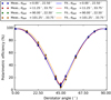 |
Fig. 3. Measured and fitted polarimetric efficiency of the instrument downstream of M4 as a function of HWP and derotator angle in the H-band. The legend only shows the |


For an ideal instrument, the polarimetric efficiency is 100%. However, in Fig. 3 a dramatic decrease in polarimetric efficiency is seen around θder = 45°, reaching values as low as 5%. This low efficiency indicates severe loss of polarization signal and is due to the derotator retardance strongly deviating from the ideal value of 180°. With 𝛥der = 99.32°, the derotator acts almost as a quarter-wave plate for which 𝛥 = 90°. Around θder = 45°, the derotator therefore produces strong crosstalk and almost all incident linearly polarized light is converted into circularly polarized light to which the P0−90 analyzer set is not sensitive. We already encountered the strongly varying polarimetric efficiency in Fig. 3 of Paper I.
The retardance of the HWP has a much smaller effect on the polarimetric efficiency than the retardance of the derotator because 𝛥HWP = 170.5° in the H-band, relatively close to the ideal value of 180°. In Fig. 3 the effect of the HWP retardance is visible as the changing skewness of the fitted curves for different HWP angles. The offset angles δHWP, δder, and δcal also contribute a small shift of the curves. Finally, the diattenuation of the polarizers d determines the maximum values of the curves around θder = 0° and θder = 90°.
The crosstalk produced by the derotator and HWP not only deteriorates the polarimetric efficiency, but also induces an offset in the measurement of the angle of linear polarization, as is illustrated by the varying Stokes Q- and U-images in Fig. 3 of Paper I. Figure 4 (of this paper) shows the measured and fitted offsets of the angle of linear polarization corresponding to the curves of Fig. 3. The offsets are computed as the actually measured angle of linear polarization (see Eq. (5)) minus the angle that would be measured in case the optical system were ideal. Figure 4 shows that the measured angle of linear polarization varies around the ideal angle, with a maximum deviation of 34° and the strongest rotation rate around θder = 45°.
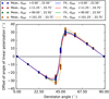 |
Fig. 4. Measured and fitted offset of the angle of linear polarization induced by the instrument downstream of M4 as a function of HWP and derotator angle in the H-band. The legend only shows the |


Figure 5 shows the polarimetric efficiency in the four broadband filters Y, J, H, and Ks. The curves displayed are for  = 0° and 22.5° and the derotator angle ranges from 0° to 180° (the curves repeat for θder > 180°). We have also taken measurements in the range 0° ≤θder ≤ 180° (not shown) that confirm the curves for θder > 90°. However, we do not use these measurements to determine the model parameters, because neutral density filters were inserted which appear to depolarize the light by a few percent. Because the nine data points of each HWP and derotator angle combination are relatively close together, we conclude that the effect of the gradient in the measured flux is small for all filters.
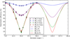 |
Fig. 5. Measured and fitted polarimetric efficiency of the instrument downstream of M4 with |


From Fig. 5 it follows that for all filters, the efficiency is minimum around θder = 45° and θder = 135°. The minimum values of the curves differ substantially among the filters, because the derotator retardance varies strongly with wavelength (see Table 1). The exact shape and minimum values of the curves depend on the HWP angles used (see Fig. 3) because the HWP retardance deviates slightly from the ideal value of 180° in all filters (strongest in the H-band; see Table 1). The asymmetry with respect to θder = 90° visible in Fig. 5 is also due to the non-ideal HWP retardance.
The absolute minimum polarimetric efficiency is lowest in the H-band for which it is 5%. Also the Ks-band (efficiency ≥7%) shows a strongly varying performance, while in the Y-band (≥54%) and especially in the J-band (≥89%) the polarimetric efficiency is much less affected by the derotator angle. The polarimetric efficiency during science observations, and an observation strategy in which the derotator angle is optimized to prevent observing at a low polarimetric efficiency are discussed in Paper I.
Figure 6 shows the offsets of the angle of linear polarization corresponding to the polarimetric efficiency curves of Fig. 5. Also in this case the non-ideal HWP retardance causes an asymmetry with respect to θder = 90° and variations of the exact shape and maximum values of the curves with HWP angle (see Fig. 4). While the variation around the ideal value is marginal in the J-band, with a maximum deviation of 4°, the offset of the angle of linear polarization is ≤11° in the Y-band and ≤34° in the H-band. For the Ks-band, the angle of linear polarization does not even return to the ideal value around θder = 45° and θder = 135°, but continues rotating beyond ±90° (where a rotation of +90° is indistinguishable from −90°).
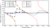 |
Fig. 6. Measured and fitted offset of angle of linear polarization induced by the instrument downstream of M4 with |


To validate the determined HWP retardances in the four filters, the values are compared to the retardance as specified by the manufacturer in Fig. 7. The error bars on the determined HWP retardances are smaller than the size of the symbols used. It follows that the determined HWP retardances are accurate, since they follow the general shape of the curve and are well within the 4% manufacturing tolerance as specified by the manufacturer2.
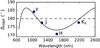 |
Fig. 7. HWP retardance as a function of wavelength as specified by the manufacturer2 compared to the determined HWP retardance (𝛥HWP) in the Y-, J-, H-, and Ks-band. |
For the unpolarized source measurements, the light incident on the HWP is primarily linearly polarized in the positive Q-direction as follows from the determined values of qin, unpol and uin, unpol. The degree of linear polarization decreases with increasing wavelength (from the Y- to Ks-band). This polarization signal must be IP from M4 that is in between the internal light source and the HWP (see Fig. 2). The determined values of qin, unpol are also in good agreement with the determined diattenuations of M4 (see Fig. 10 and the discussion in Sect. 6.2), and shows that the light from the internal light source is almost completely unpolarized until it reaches M4.
The polarization signals induced by the HWP and the derotator are very small, since ϵHWP and ϵder are very close to the ideal value of 0 in all filters (with the largest deviation for the derotator in the J-band; see Table 1). The low diattenuation of the derotator is as expected, because its main surface coating is protected silver that is highly reflective. However, considering that the derotator has its plane of incidence horizontal when θder = 0°, one would naively expect ϵder to be positive in all filters (producing polarization in the positive Q-direction) while it turns out to be negative (producing polarization in the negative Q-direction) in three of the four filters. This behavior of the diattenuation with wavelength is likely due to the complex combination of coatings on the derotator mirrors.
The strong crosstalk produced by the derotator in the H- and Ks-band can also be used to our advantage. In these filters, the retardance of the derotator is close to that of a quarter-wave plate (close to 90°; see Table 1). At θder = 45° and 135°, the derotator does not only convert almost all incident linearly polarized into circularly polarized light (problematic for the polarimetric efficiency), but it also converts almost all incident circularly polarized light into linearly polarized light that can then be measured by the P0−90 analyzer set. Hence by using the derotator as a quarter-wave plate to modulate Stokes V, we can measure circularly polarized light, for example from molecular clouds. The development of a technique to measure circularly polarized light with IRDIS is beyond the scope of this paper and is left for future work.
6. Instrumental polarization effects of telescope and M4
6.1. Calibration measurements and determination of model parameters
Now that we have a validated description of the optical path downstream of M4, we can complete our instrument model by determining the model parameters describing the UT and M4 (see Fig. 2). On June 15, 2016, we therefore observed the unpolarized standard star HD 176425 (Turnshek et al. 1990; 0.020 ± 0.009% polarized in the B-band) at different telescope altitude angles using the four broadband filters Y, J, H, and Ks under program ID 60.A-9800(S). Because M1 and M3 were re-aluminized between April 3 and April 16, 2017, we repeated the calibration measurements on August 21, 2018 with the unpolarized star HD 217343 under program ID 60.A-9801(S). Although HD 217343 is not an unpolarized standard star, it is located at only 31.8 pc from Earth (Gaia Collaboration 2018) and therefore the probability of it being polarized by interstellar dust is very low (Leroy 1993, 1999).
The two data sets are used to determine the diattenuations of the UT and M4 (ϵUT and ϵM4) before and after the re-aluminization of M1 and M3. The retardances of the UT and M4 (𝛥UT and 𝛥M4) are assumed to be equal for both data sets and are computed analytically because their limited effect does not justify dedicated calibration measurements (see Sect. 6.2). In addition the degree of linear polarization of polarized standard stars at near-infrared wavelengths is too low to accurately determine the retardances, and observations of the polarized daytime sky (see e.g. Harrington et al. 2011, 2017; de Boer et al. 2014) are very time consuming.
During the observations of HD 176425 (2016), the derotator was fixed with its plane of incidence horizontal (θder = 0°) to ensure a polarimetric efficiency close to 100%. The adaptive optics were turned off (open-loop) to reach a large total photon count per detector integration time, minimizing read-out noise. The calibration polarizer was out of the beam. For every filter, 10 HWP cycles (measurements with θHWP = 0° and 45° for Stokes Q, and with θHWP = 22.5° and 65.5° for Stokes U; see Sect. 3.1) were taken at different altitude and parallactic angle combinations. In this way, the effect of the diattenuations of the UT and M4 and a possible (but unlikely) stellar polarization signal can be distinguished when fitting the data to the model. The HWP cycles were kept short (∼140 s) to limit the parallactic and altitude angle variations of the data points themselves.
For the observations of HD 217343 (2018) we took 12 HWP cycles per filter with a similar instrument setup as used for HD 176425. The most important difference between the two setups is that this time we (accidentally) observed in field-tracking mode. In this mode the derotator is rotating continuously and therefore the polarimetric efficiency varies during the measurements. Because we did not optimize the derotator angle as recommended (see Paper I), the polarimetric efficiency reached a value as low as 31% for the last measurement in the Ks-band.
Both data sets are processed by applying dark subtraction, flat fielding, bad-pixel correction, and centering with a Moffat function as described in Paper I. Subsequently, we construct the double-difference Q- and U-images from Eq. (8) and the double-sum IQ- and IU-images from Eq. (9). Finally, we calculate the normalized Stokes parameters q and u by dividing the sum in an aperture in the Q- and U-images by the sum in the same aperture in the corresponding IQ- and IU-images (see Eq. (10)). For an elaboration on the extraction of the normalized Stokes parameters and the selected aperture sizes see Appendix D.
To describe the measurements, we use Eq. (10) with the model equations of Sect. 4 inserted (together the model function). We use the complete Eq. (17) and fill in the values of the determined parameters ϵHWP to d from Table 1. We compute the retardances of the UT (actually M3 since M1 and M2 are rotationally symmetric) and M4 using the Fresnel equations with the complex refractive index of aluminum obtained from Rakić (1995). This computation needs to be performed before determining the diattenuations, because the retardance of M4 affects the measurement of the IP produced by the UT. Because we observed unpolarized (standard) stars, we write Sin = [1, 0, 0, 0]T.
We determine the diattenuations of the UT and M4 independently for both data sets by fitting the model function to the data points using nonlinear least squares. The parallactic, altitude, HWP, and derotator angles required for this are obtained from the headers of the FITS-files of the measurements (see Appendix A). We have tested fitting the incident Stokes vectors in addition to the diattenuations (writing Sin = [1, qin, uin, 0]T), and found that the degree of linear polarization of the stars is indeed insignificant (< 0.1%) in all filters. We therefore choose not to fit the incident Stokes vectors and assume the stars to be completely unpolarized. Graphs of the model fits and the residuals can be found in Appendix D.
6.2. Results and discussion for unpolarized star calibrations
The determined diattenuations and calculated retardances of the UT and M4 for both data sets are shown in Table 2. The listed 1σ-uncertainties of the diattenuations are computed from the residuals of fit (see Appendix E) under the same assumptions as described in Sect. 5.2.
Determined diattenuations with their errors and computed retardances of the part of the model describing the telescope and M4 in the Y-, J-, H-, and Ks-band.
The calculated values of 𝛥UT and 𝛥M4 are close to the ideal value of 180° and therefore the crosstalk produced by the UT and M4 is very limited. In all filters, the combined polarimetric efficiency of the UT and M4 is > 98% and the corresponding offset of the angle of linear polarization is at most a few tenths of a degree (largest effect in the Y-band). Due to the limited crosstalk, any realistic deviation of the real retardances from the computed ones results in very small errors only. This also implies that the systematic error on ϵUT due to using an analytical rather than a measured value of 𝛥M4 is very small.
To understand the effect of the determined diattenuations, we plot the measured and fitted degree of linear polarization (see Eq. (4)) as a function of telescope altitude angle for the observations of HD 176425 (2016) and HD 217343 (2018) in Figs. 8 and 9, respectively. The degree of linear polarization can in this case be interpreted as the IP of the UT and M4. The figures also show analytical curves that are constructed by computing the diattenuations from the Fresnel equations and assuming that the aluminum coatings of the UT (M3) and M4 have the same properties. The error bars on the measurements are calculated as half the difference between the degree of linear polarization determined from apertures with radii 50 pixels larger and smaller than that used for the data points themselves (see Appendix D). The error bars show the uncertainty in the degree of linear polarization due to the dependency of the measured values on the chosen aperture radius. The uncertainty is small for all measurements except for those of HD 176425 (2016) taken in the Ks-band. The latter measurements are less certain because of difficulties in removing the thermal background signal (see Appendix D). We note that for science observations the telescope altitude angle is restricted to 30° ≤a ≤ 87°.
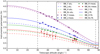 |
Fig. 8. Analytical (aluminum), measured (including error bars), and fitted instrumental polarization (IP) of the telescope and M4 as a function of telescope altitude angle in the Y-, J-, H-, and Ks-band from the measurements of HD 176425 taken in 2016 before the re-aluminization of M1 and M3. For science observations the telescope altitude angle is restricted to 30° ≤a ≤ 87°. |
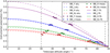 |
Fig. 9. Analytical (aluminum), measured (including error bars) and fitted instrumental polarization (IP) of the telescope and M4 as a function of telescope altitude angle in the Y-, J-, H-, and Ks-band from the measurements of HD 217343 taken in 2018 after the re-aluminization of M1 and M3. For science observations the telescope altitude angle is restricted to 30° ≤a ≤ 87°. |
Figure 8 shows that the IP increases with decreasing altitude angle and that before the re-aluminization of M1 and M3 the maximum IP (at a = 30°) is equal to approximately 3.5%, 2.5%, 1.9%, and 1.5% in the Y-, J-, H-, and Ks-band, respectively. The corresponding minimum values (at a = 87°) are 0.58%, 0.42%, 0.33%, and 0.29%, respectively. Ideally, we would expect the IP of M3 to completely cancel that of M4 when the reflection planes of the mirrors are crossed at a = 90° (analytical curves). However, because the determined ϵUT and ϵM4 are not identical, this is not the case. This discrepancy is probably caused by differences in the coating or aluminum oxide layers of the mirrors (see van Harten et al. 2009).
Figure 9 shows that the IP after the re-aluminization of M1 and M3 is significantly smaller than before. The maximum values (at a = 30°) are now equal to approximately 3.0%, 2.1%, 1.5%, and 1.3% in the Y-, J-, H-, and Ks-band, respectively, and the corresponding minimum values (at a = 87°) are 0.18%, 0.12%, 0.07%, and 0.06%, respectively. This decrease of IP is due to the lower diattenuation of the UT (see Table 2). In fact, after re-aluminization the diattenuation of the UT is comparable to that of M4, leading to almost complete cancellation of the IP at 90° altitude angle3. Because the measurements were taken in field-tracking mode, the data points shown have been corrected for the polarimetric efficiency (the residuals for the two data points in the Ks-band close to a = 30° are considerably enhanced because of this correction). Finally, during the observations of HD 217343 we did not switch filter after every HWP cycle as we did for HD 176425 (compare Figs. 8 and 9). Therefore the measurement points are less spread out over the range of altitude angles, making them constrain the model function somewhat less.
The IP created by the UT or M4 separately, as determined from the various measurements, is shown as a function of central wavelength of the Y-, J-, H-, and Ks-band in Fig. 10. The IP created is equal to the diattenuation of the mirror(s) when assuming that the incident light is completely unpolarized (see Eq. (20)). Figure 10 shows that before the re-aluminization of M1 and M3, the IP of the UT is significantly larger than that of M4 (on-sky 2016). After the re-aluminization, the IP of the UT has decreased and differs less than 0.1% from that of M4 in all filters (on-sky 2018). This indicates that the coatings of M3 and M4 are much more similar after the re-aluminization. Between the observations of the unpolarized stars in 2016 and 2018, the IP of M4 (which has not been re-aluminized) differs less than 0.07% in all filters, showing that the diattenuation does not significantly change in time.
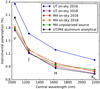 |
Fig. 10. Instrumental polarization (IP) of the UT and M4 separately, as determined from the various measurements, versus central wavelength of the Y-, J-, H-, and Ks-band. The curves show the IP of the UT and M4 from the observations of the unpolarized stars HD 176425 (on-sky 2016) and HD 217343 (on-sky 2018), the IP of M4 from the unpolarized source measurements and the IP of the UT and M4 computed from the Fresnel equations (aluminum analytical). |
Figure 10 also shows the IP of M4 as determined from the unpolarized source measurements, that is, qin, unpol from Table 1 (ignoring uin, unpol, which is close to zero in all filters). Clearly, the observations of the unpolarized stars are in good agreement with the measurements with the internal light source. The small differences among the values determined from the measurements of the unpolarized stars and the internal light source could be due to the different spectra of the stars and the internal light source, the calibration unit producing some polarization, or the finite precision of the measurements. Finally, Fig. 10 shows the IP produced by the UT or M4 as computed from the Fresnel equations (aluminum analytical). We conclude that the determined IP agrees well with the theoretical expectation.
7. Polarimetric accuracy of instrument model
In this section we determine for each broadband filter the total polarimetric accuracy of our completed instrument model and compare it to the aims we set in Sect. 1. As the first step to calculate the accuracy of the model, we compute the accuracies of fitting the model parameters to the calibration data. These accuracies of fit are calculated as the corrected sample standard deviation of the residuals in Appendix E and show the random errors of the measurements. The systematic errors of the model fits are likely small, because the residuals of fit are close to normally distributed (see Figs. C.1–C.3 and D.3–D.5).
To compute the total polarimetric accuracy from the residuals of fit, we need to compute the absolute and relative polarimetric accuracies sabs and srel (see Eqs. (11) and (12)). For the absolute polarimetric accuracy we compute separate values before and after the re-aluminization of M1 and M3. The absolute polarimetric accuracy is calculated as  , with sunpol the accuracy of fit of the unpolarized source measurements and sstar the accuracy of fit of the observations of the unpolarized star under consideration (see Appendix E). We take the relative polarimetric accuracy srel (valid before and after the re-aluminization) equal to the accuracy of fit of the polarized source measurements. The resulting absolute and relative polarimetric accuracies in the Y-, J-, H-, and Ks-band are shown in Table 3.
Absolute and relative polarimetric accuracies in the Y-, J-, H-, and Ks-band.
From Table 3 we conclude that the absolute polarimetric accuracies before and after the re-aluminization of M1 and M3 are comparable and that the requirements on the absolute and relative polarimetric accuracies (≤0.1% and < 1%, respectively) are met for all filters. The values of sabs are consistent with the ∼0.05% absolute difference among the independent estimates of the IP of M4 from the observations of the unpolarized stars and the unpolarized source measurements (see Fig. 10). Because the residuals of fit are close to normally distributed, the absolute and relative polarimetric accuracies can probably be improved by obtaining calibration measurements with a higher signal-to-noise ratio. However, the accuracy we attain when correcting science observations appears to be limited by systematic errors (see Sect. 8.4).
With the absolute and relative polarimetric accuracies calculated, we can now compute the total polarimetric accuracies in Stokes Q and U, sQ and sU, respectively, as:
 (25)
(25)
 (26)
(26)
where  ,
,  ,
,  , and
, and  are the measured Stokes IQ, IU, Q, and U incident on the telescope after correcting the instrumental polarization effects with the model (see Sect. 8.1). Equations (25) and (26) are derived from Eqs. (11) and (12) by substituting
  and
and  for the true incident Qin and Uin. We can determine the total polarimetric accuracy in the degree and angle of linear polarization (sDoLP and sAoLP) as:
 (27)
(27)
 (28)
(28)
where  ,
,  ,
,  , and
, and  . We have derived Eqs. (27) and (28) from Eqs. (4), (5), (25), and (26) by applying standard error propagation and assuming Gaussian statistics, zero uncertainty in
  and
and  , and no correlation between sQ and sU. In case
  and
and  contain substantial flux from the central star,
  ,
,  , sQ, and sU should be divided by the intensity from the source we are interested in (e.g., a circumstellar disk or substellar companion) when computing sDoLP and sAoLP. We note that corrections need to be applied to Eqs. (27) and (28) in case the signal-to-noise ratio in the degree of linear polarization is very low, that is, lower than ∼3 (see Sparks & Axon 1999; Patat & Romaniello 2006).
Table 4 shows the polarimetric accuracies of measuring the degree and angle of linear polarization of a 1% polarized substellar companion and a 30% polarized circumstellar disk in the Y-, J-, H-, and Ks-band before the re-aluminization of M1 and M3 (the results after the re-aluminization are comparable). The accuracies are computed from Eqs. (27) and (28) under the assumption that  and
and  contain no starlight. The accuracies weakly depend on the angle of linear polarization of the incident light (the specific values of
  and
and  ) and so the worst case is shown. From Table 4 it follows that for increasing degrees of linear polarization of the source, the error on the degree of linear polarization increases. For sources with a low degree of linear polarization (up to a few percent) the error is nearly equal to the absolute polarimetric accuracy sabs, while for sources with a high degree of linear polarization (several tens of percent) the contribution of the relative polarimetric accuracy srel dominates. Table 4 also shows that the error on the angle of linear polarization decreases with an increasing degree of linear polarization of the source, because the polarization components Q and U are measured with a higher relative accuracy. This also means that for sources with a very low degree of linear polarization (∼0.1%) the error on the angle of linear polarization can be as large as 10° or more.
Polarimetric accuracy of measuring the degree and angle of linear polarization of a 1% polarized substellar companion and a 30% polarized circumstellar disk in the Y-, J-, H-, and Ks-band before the re-aluminization of M1 and M3.
Assuming that Gaussian statistics apply and that systematic errors are small, Table 4 shows that the polarization signal of a 1% polarized substellar companion can be measured in all filters with the required total polarimetric accuracy of ∼0.1% in the degree of linear polarization and an accuracy of a few degrees in angle of linear polarization. For the 30% polarized circumstellar disk, the attainable accuracies in degree of linear polarization are below 0.3% in all filters, which is amply sufficient for quantitative polarimetry. For real measurements the attained accuracies are generally somewhat worse because of for example measurement noise and varying atmospheric conditions (see Sect. 8.4). In addition, the accuracy of measuring a circumstellar disk’s degree of linear polarization itself is limited by the accuracy with which the total intensity of the disk can be obtained.
8. Correction of science observations
8.1. Correction method
In this section, we explain the data-reduction method we have developed to correct science measurements for the instrumental polarization effects of the complete optical system using our instrument model. The goal of the correction method is to obtain from the measurements the  - and
- and  -images, that is, the estimates of the true Qin- and Uin-images incident on the telescope (see top right part of Fig. 2). A flow diagram of our correction method for field-tracking observations is shown in Fig. 11.
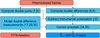 |
Fig. 11. Flow diagram showing the steps to construct the incident |


Before applying our correction method, we pre-process the raw data by performing dark subtraction, flat fielding, bad-pixel correction, and centering (see Sect. 8.2 and Paper I). Subsequently, we construct for each HWP cycle the Q- and U-images from the double difference (Eq. (8)) and the corresponding IQ- and IU-images from the double sum (Eq. (9)). We denote the n double-difference images (Q or U) by Xi and the corresponding double-sum images (IQ or IU) by IX, i, with i = 1, 2, …, n. We construct the  -and
-and  -images, that is, the IQ- and IU-images incident on the telescope, simply by computing the mean (or median) of the double-sum IQ, i- and IU, i-images, respectively.
To construct the  - and
- and  -images we use our instrument model. The instrumental polarization effects are different for each measurement, because the parallactic, altitude, HWP, and derotator angles change continuously as the telescope tracks the target. To describe these changing instrumental polarization effects, we compute the vector equivalents of the single and double difference (Eqs. (6) and (22)) using our instrument model. To this end, we obtain the date, filter, and the parallactic, altitude, HWP, and derotator angles of each measurement from the headers of the FITS-files of the data (see Appendix A). We then take the model parameters corresponding to the filter from Tables 1 (parameters ϵHWP to d) and 2, taking into account the date of the observations for the latter. For each measurement, we compute Msys, L and Msys, R from Eq. (17) using +d and −d in MCI, L/R (Eq. (21)), respectively. Similar to Sect. 4, where we computed the single difference from the top elements of Sdet, L and Sdet, R (i.e., Idet, L and Idet, R), we now compute the single difference from the top rows of Msys, L and Msys, R (which we call Isys, L and Isys, R):
 (29)
(29)
where D± is the single-difference row vector. Subsequently, we compute for every double-difference image Xi the double-difference row vector Di as:
![Mathematical equation: $$ \begin{aligned} \boldsymbol{D}_i&= \dfrac{1}{2} \left[\boldsymbol{D}^+\left(p_i^+, a_i^+, \theta _{\mathrm{HWP} ,i}^+, \theta _{\mathrm{der} ,i}^+ \right) - \boldsymbol{D}^-\left(p_i^-, a_i^-, \theta _{\mathrm{HWP} ,i}^-, \theta _{\mathrm{der} ,i}^-\right)\right], \nonumber \\&= \begin{bmatrix} (I \rightarrow X)_i&(Q \rightarrow X)_i&(U \rightarrow X)_i&(V \rightarrow X)_i \end{bmatrix}, \end{aligned} $$](/articles/aa/full_html/2020/01/aa34996-18/aa34996-18-eq85.gif) (30)
(30)
where D+ and D− are a function of the parallactic, altitude, HWP, and derotator angles of the first (superscript +) and second (superscript −) measurements used to compute the double difference, respectively.
To describe the ith double-difference measurement, we can write:
 (31)
(31)
We can ignore the element (V → X)i, that is, assume Vin = 0, because we do not expect circularly polarized signals from the targets we are interested in. In addition, we can assume that the measured double-sum intensities IX, i are equal to the incident intensity Iin (the resulting maximum relative error is ∼10−4). Therefore, we can describe the ith double-difference measurement as:
 (32)
(32)
The elements (I → X)i describe the instrumental polarization (IP) of the complete optical system for each measurement. We remove the IP from each double-difference image Xi by scaling the corresponding double-sum intensity image IX, i with this element and subtracting the result from the double-difference image:
 (33)
(33)
where XIPS, i is the ith IP-subtracted double-difference image.
The elements (Q → X)i and (U → X)i in Eq. (32) account for the crosstalk (and thus for the polarimetric efficiency and offset of the angle of linear polarization) of the complete optical system for each measurement. To correct for the crosstalk, we set up a system of equations as follows:
![Mathematical equation: $$ \begin{aligned}&\boldsymbol{Y} = A \left[Q_\mathrm{in} , U_\mathrm{in} \right]^\mathrm{T} , \nonumber \\&\begin{bmatrix} X_{\mathrm{IPS} ,1} \\ X_{\mathrm{IPS} ,2} \\ \vdots \\ X_{\mathrm{IPS} ,n} \end{bmatrix}= \begin{bmatrix} (Q \rightarrow X)_1&(U \rightarrow X)_1 \\ (Q \rightarrow X)_2&(U \rightarrow X)_2 \\ \vdots&\vdots \\ (Q \rightarrow X)_n&(U \rightarrow X)_n \end{bmatrix} \begin{bmatrix} Q_\mathrm{in} \\ U_\mathrm{in} \end{bmatrix}, \end{aligned} $$](/articles/aa/full_html/2020/01/aa34996-18/aa34996-18-eq89.gif) (34)
(34)
with Y a column vector containing the i = 1, 2, …, n IP-subtracted double-difference images, Qin and Uin the true Q- and U-images incident on the telescope and A the n × 2 system matrix containing the elements (Q → X)i and (U → X)i of each double difference. We obtain the  - and
- and  -images, that is, the estimates of the true incident Qin- and Uin-images, by solving for every pixel the system of equations using linear least squares:
![Mathematical equation: $$ \begin{aligned} \left[\hat{Q}_\mathrm{in} , \hat{U}_\mathrm{in} \right]^\mathrm{T} = (A^\mathrm{T} A)^{-1} A^\mathrm{T} \boldsymbol{Y}. \end{aligned} $$](/articles/aa/full_html/2020/01/aa34996-18/aa34996-18-eq92.gif) (35)
(35)
Alternatively, we can obtain the incident  - and
- and  -images by solving the system of equations for each pair of IP-subtracted double-difference Q- and U-images (each HWP cycle) separately, and then computing the median or trimmed mean over all resulting
  - and
- and  -images. Computing the median or trimmed mean has the advantage that any bad pixels still visible in the images are removed, but using Eq. (35) is expected to generally yield more accurate results. In place of Eq. (35) we can also use weighted linear least squares, wherein the weight matrix takes into account the signal-to-noise ratio of the images or the polarimetric efficiency as predicted by the instrument model. We note that the correction method (using Eq. (35)) can be applied to data sets having an unequal number of double-difference Q and U measurements.
The instrument model is valid for any combination of parallactic, altitude, HWP, and derotator angles and does not require the use of a particular rotation control law for the HWP and derotator. However, for observations not taken in field-tracking mode (e.g., pupil-tracking mode), the derotator does not keep the image orientation constant. We therefore need to derotate with our pipeline the images after subtracting the IP and before correcting the crosstalk. The adapted correction method for pupil-tracking observations, which in addition combines polarimetry with angular differential imaging (ADI), is presented in van Holstein et al. (2017).
8.2. Correction of images of circumstellar disk of T Cha
The correction method presented in Sect. 8.1 has already been successfully applied to over a hundred polarimetric data sets, including HR 8799 and PZ Tel (van Holstein et al. 2017), TW Hydrae (Paper I), T Cha (Pohl et al. 2017a), DZ Cha (Canovas et al. 2018), TWA7 (Olofsson et al. 2018), PDS 70 (Keppler et al. 2018), and CS Cha (Ginski et al. 2018). In this section, we demonstrate our correction method with the H-band polarimetric observations of the circumstellar disk of T Chamaeleontis (T Cha) as published in Pohl et al. (2017a). The transition disk around T Cha consists of a coplanar inner and outer disk separated by a large gap, and is viewed close to edge-on with an inclination of ∼69° (Olofsson et al. 2013; Pohl et al. 2017a; Hendler et al. 2018). While the outer disk can easily be spatially resolved with SPHERE, the very narrow and close-in inner disk cannot (its extent is only < 0.2 pixel on the IRDIS detector).
The data of T Cha was taken on February 20, 2016 under program ID 096.C-0248(C). It consists of a total of 30 HWP cycles with HWP switch angles 0°, 45°, 22.5°, and 65.5° to measure Stokes Q and U (see Sect. 3.1). During the observations, the parallactic and altitude angles varied from 5.8° to 27.3°, and from 35.1° to 34.1°, respectively. We pre-process the raw data by performing dark subtraction, flat fielding, bad-pixel correction, and centering with the star center frames as described in Paper I and Pohl et al. (2017a). We then construct the Q- and U-images from the double difference (Eq. (8)) and the IQ- and IU-images from the double sum (Eq. (9)). The Q- and U-images show a weak detector artifact comprised of continuous vertical bands. We remove this artifact by subtracting, for every pixel column, the median value of the 60 pixels at the top and bottom of that column (see Paper I). The resulting double-difference U-images of the first and last (30th) HWP cycle are shown in the left column of Fig. 12. The pronounced differences between the two images are predominantly caused by IP that evolves from negative to positive U during the 78 min total observing time.
 |
Fig. 12. Effect of the data-reduction steps of our correction method on the Stokes U-images of the first and last (30th) HWP cycle of the observations of the circumstellar disk of T Cha. |
We now apply our correction method (using the diattenuations of the UT and M4 valid before April 16, 2017) and subtract the IP from the double-difference Q- and U-images (see Eq. (33)). The resulting IP-subtracted U-images of the first and last HWP cycle are shown in the center column of Fig. 12. The resulting images are much more similar compared to the original double-difference images (left column). However, the optical system’s crosstalk makes the disk brighter in Stokes U and fainter in Stokes Q during the course of the observations. This is because the crosstalk transfers part of the flux in Stokes Q to Stokes U or vice versa, that is, it introduces an offset in the angle of linear polarization (see Fig. 4). In addition the crosstalk converts part of the linearly polarized light into circularly polarized light that the P0−90 analyzer set is not sensitive to, entailing a loss of signal as quantified by the polarimetric efficiency (see Fig. 3). These two effects are also seen in Fig. 3 of Paper I as variations in the Stokes Q- and U-images. Although the polarimetric efficiency during the observations of T Cha is not very low (minimum of 88%), the offset of the angle of linear polarization reaches values as large as 13°. This shows that even for observations taken at a reasonably high polarimetric efficiency, there is still significant transfer of signal between the Stokes Q- and U-images (we recall that the orientations of Q and U differ by 45°).
We correct for the crosstalk using linear least squares (see Eq. (35)), directly yielding the  - and
- and  -images. The right column of Fig. 12 shows the resulting
  -images of the first and last HWP cycle after solving the system of equations for each HWP cycle separately. It follows that after crosstalk correction the disk has a very similar surface brightness distribution in all images. The integrated signal of the disk only varies by a few percent among the images, which is due to varying atmospheric conditions during the observations (e.g., seeing and sky transparency). Although by correcting the crosstalk we compensate for the polarimetric efficiency, this does not increase the signal-to-noise ratio (as clearly visible in Fig. 8 of Paper I). Next, we subtract the constant polarized background in the
  - and
- and  -images after determining it from a large star-centered annulus with inner and outer radii of 360 and 420 pixels, respectively. Finally, we use the resulting images and Eqs. (3) and (5) to compute the polarized intensity and angle of linear polarization of the disk as shown in Fig. 13.
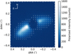 |
Fig. 13. Polarized intensity and angle of linear polarization of the circumstellar disk of T Cha after applying the correction method. The white lines indicating the angle of linear polarization have arbitrary length and are only shown where the polarized intensity is higher than 50 counts. |
8.3. Improvements attained with correction method
In this section we show the improvements attained with our correction method by comparing the model-corrected  - and
- and  -images of T Cha with Q- and U-images generated with the conventional IP-subtraction method as presented by Canovas et al. (2011). In Paper I we made a similar comparison using data of the (nearly) face-on viewed disk of TW Hydrae. While that data set could in principle be reduced using conventional data-reduction methods, in this section we show that the correction method is essential to accurately reduce data of an inclined disk and that it enables us to detect non-azimuthal polarization and the polarization of the starlight.
To construct the Q- and U-images with the conventional IP-subtraction method, we compute the mean of the double-difference Q- and U- and double-sum IQ- and IU-images, and subtract the IP following the steps described in Sect. 4.1 of Paper I. We convert these and the model-corrected images into images of the azimuthal Stokes parameters Qϕ and Uϕ (see Sect. 4.2 and Eqs. (15)–(17) of Paper I) to ease the comparison and interpretation of the images. The resulting images are shown in Fig. 14.
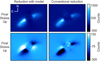 |
Fig. 14. Final azimuthal Stokes Qϕ- and Uϕ-images of the circumstellar disk of T Cha after applying our correction method compared to the images generated with the conventional IP-subtraction method from Canovas et al. (2011). Positive Qϕ indicates linear polarization in the azimuthal direction and Uϕ shows the linear polarization at ±45° from this direction. The color scales of the top and bottom row are different, i.e., the signals in Qϕ are almost 10 times larger than the signals in Uϕ. |
The model-corrected images are more accurate than the images generated with the conventional IP-subtraction method. With our correction method the instrumental polarization effects are known a priori and are corrected with an absolute polarimetric accuracy of ∼0.1% or better (see Table 3 and Sect. 8.4). The conventional IP-subtraction method on the other hand does not correct the crosstalk and estimates the IP from the science data under the assumption that the starlight is unpolarized, resulting in errors in the polarized intensity and angle of linear polarization.
Comparing the left and right columns of Fig. 14, it follows that the disk in the model-corrected Qϕ-image is ∼20% brighter. This increase in brightness is largely due to the crosstalk correction, that is, the correction of the polarimetric efficiency and transfer of signal between the Qϕ- and Uϕ-images (or Q- and U-images). As a result of the correction, the polarized surface brightness distribution, orientation and morphology of the disk are more accurately retrieved in the model-corrected images.
Figure 14 also shows that both reduction methods yield non-zero Uϕ-signals, but with significant differences. Our correction method corrects for the IP and crosstalk without an assumption on the polarization of the star (as in the conventional IP-subtraction method) or the angle of linear polarization over the disk (as in the Uϕ-minimization method, see Paper I). Therefore our correction method is truly sensitive to non-azimuthal polarization and yields the accurate Uϕ-image. From Fig. 13 and the model-corrected Uϕ-image of Fig. 14, we can conclude that away from the brightness region of the disk the angle of linear polarization deviates from the azimuthal direction. Pohl et al. (2017a) primarily attribute this non-azimuthal polarization to multiple scattering starting in the inner disk.
A clear disadvantage of the conventional IP-subtraction method is that it substantially over-subtracts the IP when the star is polarized, because it cannot discern IP from polarized starlight. Figure 15 shows for each individual HWP cycle the polarization signal as measured from the AO residuals in the model-corrected  - and
- and  -images. The figure shows that the measured polarization signal, and therefore the angle of linear polarization, is constant in time. This indicates that the starlight is polarized, because any uncorrected IP would have changed with the variation in parallactic and altitude angle during the observations.
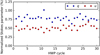 |
Fig. 15. Normalized Stokes parameters of the measured stellar polarization of T Cha as function of HWP cycle after applying our correction method. |
From Fig. 15, and using the variation in the data points for the uncertainties, we find that the star has a degree and angle of linear polarization of 0.94 ± 0.07% and 17 ± 2°, respectively. This stellar polarization signal is most likely not caused by interstellar dust, because T Cha is located in front of, and not in, the Cha I dark cloud (Murphy et al. 2013; Gaia Collaboration 2018) and the angle of linear polarization differs by ∼80° with respect to the average in the cloud (Covino et al. 1997). Because the measured angle of linear polarization is approximately perpendicular to the position angle of the outer circumstellar disk (see the top left image of Fig. 13), the stellar polarization signal most likely originates from the coplanar, spatially unresolved inner disk and/or part of the outer disk viewed close to the star. Indeed, the model-corrected images of Fig. 14, which still contain the stellar polarization signal, correspond much better to radiative transfer models than the images generated with the conventional IP-subtraction method (see Pohl et al. 2017a; also Keppler et al. 2018).
It appears to be quite common for stars that host a circumstellar disk to be polarized, because in at least half of the more than hundred data sets we have applied our correction method to we measure significant stellar polarization. If interstellar dust can be excluded as the origin, the stellar polarization can indicate the presence of a spatially unresolved (inner) disk, in particular for a circumstellar disk with a low to moderate inclination (see e.g., Keppler et al. 2018). The position angle of an inner disk can then be determined from the measured angle of linear polarization. For a detailed example on how to determine whether the stellar polarization is caused by interstellar dust, see Ginski et al. (2018). We note that to measure the small polarization signals of substellar companions, measuring the polarization of the star is imperative to prove that the companion’s polarization is intrinsic and is not caused by over-subtraction of disk-induced stellar polarization or interstellar dust.
8.4. Limits to and optimization of polarimetric accuracy
The polarimetric accuracy of measuring Stokes Q and U and the degree and angle of linear polarization after applying our correction method can be computed from Eqs. (25)–(28). However, with real measurements the uncertainty on these physical quantities is generally somewhat worse than the computed accuracies. The accuracies of Table 3 should therefore be considered lower limits. In general, for stars that are not polarized because of their circumstellar disk or interstellar dust, a polarization signal of ∼0.1% remains after applying our correction method. The higher uncertainty on the measured polarization is likely due to limitations of the instrument model, measurement noise, and varying atmospheric conditions. In this section we elaborate on these limiting factors and discuss means to optimize the polarimetric accuracy.
A first limitation of the instrument model is that we assume the instrumental polarization effects to be fixed for a given broadband filter. However, because the instrumental polarization effects vary with wavelength (see e.g., Figs. 5 and 8), any spectral differences between the science object and the calibration sources used to determine the model parameters introduce small errors in the correction of the IP and crosstalk. We can limit these errors by comparing the spectra of the science object and calibration sources and interpolating the values of the model parameters over the wavelength domain. Such an interpolation is quite accurate for the diattenuations of the UT and M4 and the retardance of the HWP, because their spectral dependency is smooth and is known from theory and the manufacturer, respectively (see e.g., Fig. 7). The largest interpolation errors are expected for the retardance of the derotator, because we need to guess the shape of the function from the four measured data points. By interpolating the model parameters we are also able to correct measurements taken with the narrowband filters.
A second limitation of the instrument model is that the instrumental polarization effects are taken constant over the field of view. We know the instrumental polarization effects have spatial dependence, because the images of the internal calibration measurements display a gradient (see Appendix B). However, contrary to the polarimetric imaging mode of FORS (Patat & Romaniello 2006), this spatial dependence is very small as demonstrated by the relative proximity of the nine data points taken throughout the image for each HWP and derotator angle combination in Figs. 3–6 and C.1–C.3. The main reason for the limited spatial dependence is that the light beams within SPHERE have much larger f-numbers than those within FORS, that is, the beams converge and diverge much more slowly within SPHERE. Because we have determined the model parameters from all these data points together (see Sect. 5.1), the spatial dependence downstream of M4 is accounted for in the polarimetric accuracy of the model. Nevertheless, we can increase the accuracy of the model by determining a separate set of model parameters from each of the nine apertures used, because the nine data points do not vary randomly around their average value but show a relation with position on the detector. We do not expect the diattenuations and retardances of the UT and M4 to be strongly spatially dependent, because spatial variations generally originate from transmissive optics near a focal plane.
A third limitation of the model is that the instrumental polarization effects are assumed to be constant in time. At least some temporal variation is expected for the diattenuation and retardance of the UT, because the UT is open to the atmosphere and therefore the amount of contamination (e.g., dust) on the mirrors varies (see Snik & Keller 2013). However, as M1 and M3 are cleaned with CO2 on a monthly basis, this variation is most likely small. For the other optical components we do not expect temporal variations due to contamination because they are located within SPHERE. Aging of these components is most likely also limited, because the model parameters describing the optical path downstream of M4 seem not to have changed since the internal calibration measurements of 2016, and the determined diattenuation of M4 has not significantly changed between the observations of the unpolarized stars in 2016 and 2018 (see Sect. 6.2). To optimize the accuracy of our correction, we can recalibrate the diattenuation of the UT and M4 during the same night as the science observations, preferably with an unpolarized star that has a spectrum as similar as possible to that of the science object(s).
To keep the instrument model accurate over time, new calibration measurements need to be taken when a modification is made to the optical path that affects the polarimetry. Examples of such modifications are the insertion of a new optical component, the replacement or removal of an existing component, or the re-coating of a mirror (e.g., the re-aluminization of M1 and M3 as performed between April 3 and April 16, 2017). Because the mathematical description of our model includes the double difference, changes to the optical path downstream of the derotator generally do not require new calibration measurements.
The polarimetric accuracy we can really attain is also affected by measurement noise. In Eq. (11), the polarimetric accuracy is defined for infinite sensitivity, that is, without any noise or spurious signals present in the data. However, in general the combined photon, speckle, (sky) background, and read-out noise of a measurement is much larger than the polarimetric accuracy of the instrument model. Therefore, when stating uncertainties of measured polarization signals, we recommend to always compare the polarimetric accuracy as computed from Eqs. (25)–(28) with the measurement noise. The criteria to reach a polarimetric sensitivity, in addition to a polarimetric accuracy, of ≤0.1% with IRDIS for the measurement of polarization signals of substellar companions are discussed in van Holstein et al. (2017).
With the double-difference method, spurious polarization signals created when the atmospheric seeing or sky transparency changes between measurements is removed to first order. Some spurious signals remain, because these atmospheric variations prevent the effect of the diattenuation of the components downstream from the derotator to be completely removed. When the variations in seeing and sky transparency are large, the spurious signals can be suppressed by computing Stokes Q and U from the “normalized” double difference (compare to Eq. (8)):
 (36)
(36)
with IX computed from Eq. (9).
The accurate polarized intensity images that we obtain with our correction method enable the construction of images of the degree of linear polarization of circumstellar disks. To construct such an image, an image of the total intensity of the disk is required. In principle such an image can be obtained by subtracting the point spread function of a reference star (e.g., Canovas et al. 2013) or by using angular differential imaging for disks seen close to edge-on (e.g., Perrin et al. 2015). However, these techniques have proven to be challenging and residual speckles from the star remain in the total intensity image of the disk. Therefore the accuracy of measuring the degree of linear polarization of circumstellar disks is limited by the accuracy of the total intensity image rather than the accuracy of the instrument model.
8.5. Data-reduction pipeline including correction method
We have incorporated our correction method in a highly-automated end-to-end data-reduction pipeline called IRDAP (IRDIS Data reduction for Accurate Polarimetry). IRDAP is publicly available and handles data taken both in field- and pupil-tracking mode and using the broadband filters Y, J, H, and Ks. Data taken with the narrowband filters can be reduced as well, although with a lower accuracy, by using the correction method of the broadband filters. For pupil-tracking observations IRDAP can additionally apply angular differential imaging.
Reducing data with IRDAP is very straightforward and does not require the user to do any coding. IRDAP is simply run from a terminal with only a few commands and uses a configuration file with a limited number of input parameters. For an average-sized data set and using a modern computer, IRDAP performs a complete data reduction from raw data to final data products within a few minutes.
The documentation of IRDAP, including the installation and user instructions, can be found online4. We plan to regularly add functionalities and make improvements to IRDAP. Among others, we plan to calibrate the instrument in the narrowband filters to also enable the accurate reduction of data taken in these filters.
9. Summary and conclusions
We have created a detailed Mueller matrix model describing the instrumental polarization effects of the Unit Telescope (UT) and SPHERE/IRDIS in the broadband filters Y, J, H, and Ks. To determine the parameters of the model, we have taken measurements with SPHERE’s internal light source and have observed two unpolarized stars. We have developed a data-reduction method that uses the model to correct for the instrumental polarization and crosstalk. We have exemplified this correction method with observations of the circumstellar disk of T Cha and have shown the improvements compared to conventional data-reduction and analysis methods.
The instrumental polarization (IP) of the optical system primarily originates from the UT and SPHERE’s first mirror (M4) and increases with decreasing telescope altitude angle. The IP is different for observations taken before and after the re-aluminization of the primary and tertiary mirrors of the UT (M1 and M3). Before the re-aluminization (i.e., before April 16, 2017), the maximum IP (at an altitude angle of 30°) is approximately equal to 3.5%, 2.5%, 1.9%, and 1.5% in the Y-, J-, H-, and Ks-band, respectively. After the re-aluminization (i.e., after April 16, 2017), the maximum IP in the same filters is approximately 3.0%, 2.1%, 1.5%, and 1.3%, respectively.
The crosstalk of the optical system is strongly wavelength dependent and is primarily produced by the derotator (K-mirror). The crosstalk decreases the polarimetric efficiency, because it converts linearly polarized light into circularly polarized light that IRDIS cannot measure. The polarimetric efficiency is lowest when the reflection plane of the derotator is at approximately ±45° from the vertical direction and has minimum values equal to 54%, 89%, 5%, and 7% in the Y-, J-, H-, and Ks-band, respectively. The crosstalk also causes an offset of the angle of linear polarization in these filters, with maximum deviations equal to 11°, 4°, 34°, and 90°, respectively. In Paper I, we present a strategy to prevent observing at a low polarimetric efficiency by optimizing the derotator angle.
In all broadband filters, the instrument model has an absolute and relative polarimetric accuracy of ≤0.1% and < 1%, respectively. With these accuracies we can measure the polarization signals of substellar companions with a total polarimetric accuracy of ∼0.1% in the degree of linear polarization and an accuracy of a few degrees in angle of linear polarization. These accuracies are amply sufficient for quantitative polarimetry of circumstellar disks, because these objects are typically polarized a few tens of percent. The uncertainty on the measured polarization after applying our correction method to science observations is generally somewhat worse than the accuracies of the model itself due to limitations of the model, varying atmospheric conditions, and measurement noise.
With our correction method the IP and crosstalk are known a priori and for weakly polarized sources are corrected with an absolute polarimetric accuracy of ∼0.1% or better. This is contrary to conventional data-reduction methods that do not correct the crosstalk and estimate the IP from the (noisy) science data. Using our correction method we can therefore more accurately measure the polarized intensity and angle of linear polarization. With the correction method we can also measure the polarization of the star, which enables us to detect spatially unresolved (inner) disks and prove that the measured polarization signal of a substellar companion is intrinsic to the companion. The method can be applied to measurements taken both in field- and pupil-tracking mode.
We have incorporated our correction method in a highly-automated end-to-end data-reduction pipeline called IRDAP (IRDIS Data reduction for Accurate Polarimetry). IRDAP is publicly available and the documentation, including the installation and user instructions, can be found online5. To achieve the highest polarimetric accuracy, it is recommended to always use IRDAP for the reduction of IRDIS polarimetric data. Even for observations of nearly face-on circumstellar disks or measurements taken at a high polarimetric efficiency (e.g., when the derotator is kept at a favorable angle or observations are performed in the J-band), our correction method makes a significant correction to the angle of linear polarization and increases the signal-to-noise ratio in the final images.
For pupil-tracking observations this is true since January 22, 2019, when the new HWP rotation law was implemented (see also van Holstein et al. 2017).
B. Halle Nachfl. GmbH, http://www.b-halle.de/products/Retarders/Achromatic_Retarders.html, consulted November 21, 2017.
ZIMPOL (Schmid et al. 2018), the visible imaging polarimeter of SPHERE, has an additional HWP in between M3 and M4 that is used to rotate the IP produced by M3 such that it is ideally completely canceled by M4 at any altitude angle (Roelfsema et al. 2010). However, also at visible wavelengths the diattenuations of M3 and M4 were probably not equal before the re-aluminization of M1 and M3, so that some IP originating from the UT and M4 must have remained for ZIMPOL. After the re-aluminization, the IP of ZIMPOL is most likely close to zero because the diattenuations are much more comparable.
Acknowledgments
A significant part of this work was performed when RGvH, JHG and JdB were affiliated to ESO. RGvH and JdB thank ESO for the studentship at ESO Santiago during which this project was started. Many thanks go out to the SPHERE team and the instrument scientists and operators of the ESO Paranal observatory for their support during the calibration measurements. The research of JdB and FS leading to these results has received funding from the European Research Council under ERC Starting Grant agreement 678194 (FALCONER). This research has made use of the SIMBAD database, operated at the CDS, Strasbourg, France. This research has made use of NASA’s Astrophysics Data System Bibliographic Services. SPHERE is an instrument designed and built by a consortium consisting of IPAG (Grenoble, France), MPIA (Heidelberg, Germany), LAM (Marseille, France), LESIA (Paris, France), Laboratoire Lagrange (Nice, France), INAF – Osservatorio di Padova (Italy), Observatoire de Genève (Switzerland), ETH Zurich (Switzerland), NOVA (Netherlands), ONERA (France), and ASTRON (Netherlands) in collaboration with ESO. SPHERE was funded by ESO, with additional contributions from the CNRS (France), MPIA (Germany), INAF (Italy), FINES (Switzerland) and NOVA (Netherlands). SPHERE also received funding from the European Commission Sixth and Seventh Framework Programs as part of the Optical Infrared Coordination Network for Astronomy (OPTICON) under grant number RII3-Ct-2004-001566 for FP6 (2004−2008), grant number 226604 for FP7 (2009−2012), and grant number 312430 for FP7 (2013−2016).
References
- Bagnulo, S., Landolfi, M., Landstreet, J. D., et al. 2009, PASP, 121, 993 [Google Scholar]
- Bass, M., Stryland, E. W. V., Williams, D. R., & Wolfe, W. L. 1995, Handbook of Optics Volume II Devices, Measurements, and Properties 2nd edition (New York: McGraw-Hill, Inc.) [Google Scholar]
- Beck, C., Schlichenmaier, R., Collados, M., Bellot Rubio, L., & Kentischer, T. 2005, A&A, 443, 1047 [NASA ADS] [CrossRef] [EDP Sciences] [Google Scholar]
- Beuzit, J. L., Vigan, A., Mouillet, D., et al. 2019, A&A, 631, A155 [NASA ADS] [CrossRef] [EDP Sciences] [Google Scholar]
- Canovas, H., Rodenhuis, M., Jeffers, S. V., Min, M., & Keller, C. U. 2011, A&A, 531, A102 [NASA ADS] [CrossRef] [EDP Sciences] [Google Scholar]
- Canovas, H., Ménard, F., Hales, A., et al. 2013, A&A, 556, A123 [NASA ADS] [CrossRef] [EDP Sciences] [Google Scholar]
- Canovas, H., Ménard, F., de Boer, J., et al. 2015, A&A, 582, L7 [NASA ADS] [CrossRef] [EDP Sciences] [Google Scholar]
- Canovas, H., Montesinos, B., Schreiber, M. R., et al. 2018, A&A, 610, A13 [NASA ADS] [CrossRef] [EDP Sciences] [Google Scholar]
- Carbillet, M., Bendjoya, P., Abe, L., et al. 2011, Exp. Astron., 30, 39 [Google Scholar]
- Covino, E., Palazzi, E., Penprase, B. E., Schwarz, H. E., & Terranegra, L. 1997, A&AS, 122, 95 [NASA ADS] [CrossRef] [EDP Sciences] [Google Scholar]
- de Boer, J., Girard, J. H., Mawet, D., et al. 2014, in Ground-based and Airborne Instrumentation for Astronomy V, Proc. SPIE, 9147, 914787 [Google Scholar]
- de Boer, J., Salter, G., Benisty, M., et al. 2016, A&A, 595, A114 [NASA ADS] [CrossRef] [EDP Sciences] [Google Scholar]
- de Boer, J., Langlois, M., van Holstein, R. G., et al. 2020, A&A, 633, A63 [NASA ADS] [CrossRef] [EDP Sciences] [Google Scholar]
- de Kok, R. J., Stam, D. M., & Karalidi, T. 2011, ApJ, 741, 59 [Google Scholar]
- Dohlen, K., Langlois, M., Saisse, M., et al. 2008, in Ground-based and Airborne Instrumentation for Astronomy II, Proc. SPIE, 7014, 70143L [Google Scholar]
- Fusco, T., Rousset, G., Sauvage, J.-F., et al. 2006, Opt. Exp., 14, 7515 [Google Scholar]
- Gaia Collaboration (Brown, A. G. A., et al.) 2018, A&A, 616, A1 [NASA ADS] [CrossRef] [EDP Sciences] [Google Scholar]
- Garufi, A., Benisty, M., Stolker, T., et al. 2017, The Messenger, 169, 32 [NASA ADS] [Google Scholar]
- Ginski, C., Stolker, T., Pinilla, P., et al. 2016, A&A, 595, A112 [NASA ADS] [CrossRef] [EDP Sciences] [Google Scholar]
- Ginski, C., Benisty, M., van Holstein, R. G., et al. 2018, A&A, 616, A79 [NASA ADS] [CrossRef] [EDP Sciences] [Google Scholar]
- Gratadour, D., Rouan, D., Grosset, L., Boccaletti, A., & Clénet, Y. 2015, A&A, 581, L8 [NASA ADS] [CrossRef] [EDP Sciences] [Google Scholar]
- Guerri, G., Daban, J.-B., Robbe-Dubois, S., et al. 2011, Exp. Astron., 30, 59 [Google Scholar]
- Harrington, D. M., Kuhn, J. R., & Hall, S. 2011, PASP, 123, 799 [CrossRef] [Google Scholar]
- Harrington, D. M., Kuhn, J. R., & Ariste, A. L. 2017, J. Astron. Telesc. Instrum. Syst., 3, 018001 [NASA ADS] [CrossRef] [Google Scholar]
- Hendler, N. P., Pinilla, P., Pascucci, I., et al. 2018, MNRAS, 475, L62 [Google Scholar]
- Hugot, E., Ferrari, M., El Hadi, K., et al. 2012, A&A, 538, A139 [NASA ADS] [CrossRef] [EDP Sciences] [Google Scholar]
- Ichimoto, K., Lites, B., Elmore, D., et al. 2008, Sol. Phys., 249, 233 [Google Scholar]
- Jensen-Clem, R., Millar-Blanchaer, M., Mawet, D., et al. 2016, ApJ, 820, 111 [Google Scholar]
- Keller, C. U. 2002, in Astrophysical Spectropolarimetry, eds. J. Trujillo-Bueno, F. Moreno-Insertis, & F. Sánchez, 303 [Google Scholar]
- Keppler, M., Benisty, M., Müller, A., et al. 2018, A&A, 617, A44 [NASA ADS] [CrossRef] [EDP Sciences] [Google Scholar]
- Langlois, M., Dohlen, K., Vigan, A., et al. 2014, in Ground-based and Airborne Instrumentation for Astronomy V, Proc. SPIE, 9147, 91471R [Google Scholar]
- Leroy, J. L. 1993, A&A, 274, 203 [NASA ADS] [Google Scholar]
- Leroy, J. L. 1999, A&A, 346, 955 [NASA ADS] [Google Scholar]
- Maire, A. L., Langlois, M., Dohlen, K., et al. 2016, in Ground-based and Airborne Instrumentation for Astronomy VI, Proc. SPIE, 9908, 990834 [Google Scholar]
- Marley, M. S., & Sengupta, S. 2011, MNRAS, 417, 2874 [Google Scholar]
- Marois, C., Lafrenière, D., Doyon, R., Macintosh, B., & Nadeau, D. 2006, ApJ, 641, 556 [Google Scholar]
- Millar-Blanchaer, M. A., Graham, J. R., Pueyo, L., et al. 2015, ApJ, 811, 18 [Google Scholar]
- Millar-Blanchaer, M. A., Perrin, M. D., Hung, L. W., et al. 2016, in Ground-based and Airborne Instrumentation for Astronomy VI, Proc. SPIE, 9908, 990836 [Google Scholar]
- Milli, J., Mawet, D., Pinte, C., et al. 2015, A&A, 577, A57 [NASA ADS] [CrossRef] [EDP Sciences] [Google Scholar]
- Milli, J., Vigan, A., Mouillet, D., et al. 2017, A&A, 599, A108 [NASA ADS] [CrossRef] [EDP Sciences] [Google Scholar]
- Min, M., Dullemond, C. P., Dominik, C., de Koter, A., & Hovenier, J. W. 2009, A&A, 497, 155 [NASA ADS] [CrossRef] [EDP Sciences] [Google Scholar]
- Min, M., Canovas, H., Mulders, G. D., & Keller, C. U. 2012, A&A, 537, A75 [NASA ADS] [CrossRef] [EDP Sciences] [Google Scholar]
- Murphy, S. J., Lawson, W. A., & Bessell, M. S. 2013, MNRAS, 435, 1325 [Google Scholar]
- Muto, T., Grady, C. A., Hashimoto, J., et al. 2012, ApJ, 748, L22 [Google Scholar]
- Olofsson, J., Benisty, M., Le Bouquin, J.-B., et al. 2013, A&A, 552, A4 [NASA ADS] [CrossRef] [EDP Sciences] [Google Scholar]
- Olofsson, J., van Holstein, R. G., Boccaletti, A., et al. 2018, A&A, 617, A109 [NASA ADS] [CrossRef] [EDP Sciences] [Google Scholar]
- Patat, F., & Romaniello, M. 2006, PASP, 118, 146 [Google Scholar]
- Perrin, M. D., Schneider, G., Duchene, G., et al. 2009, ApJ, 707, L132 [Google Scholar]
- Perrin, M. D., Duchene, G., Millar-Blanchaer, M., et al. 2015, ApJ, 799, 182 [Google Scholar]
- Pinte, C., Harries, T. J., Min, M., et al. 2009, A&A, 498, 967 [NASA ADS] [CrossRef] [EDP Sciences] [Google Scholar]
- Pohl, A., Sissa, E., Langlois, M., et al. 2017a, A&A, 605, A34 [NASA ADS] [CrossRef] [EDP Sciences] [Google Scholar]
- Pohl, A., Benisty, M., Pinilla, P., et al. 2017b, ApJ, 850, 52 [Google Scholar]
- Quanz, S. P., Avenhaus, H., Buenzli, E., et al. 2013, ApJ, 766, L2 [Google Scholar]
- Rakić, A. D. 1995, Appl. Opt., 34, 4755 [CrossRef] [Google Scholar]
- Roelfsema, R., Schmid, H. M., Pragt, J., et al. 2010, in Ground-based and Airborne Instrumentation for Astronomy III, Proc. SPIE, 7735, 77354B [NASA ADS] [Google Scholar]
- Schmid, H. M., Bazzon, A., Roelfsema, R., et al. 2018, A&A, 619, A9 [NASA ADS] [CrossRef] [EDP Sciences] [Google Scholar]
- Skumanich, A., Lites, B. W., Pillet, V. M., & Seagraves, P. 1997, ApJS, 110, 357 [NASA ADS] [CrossRef] [Google Scholar]
- Snik, F., & Keller, C. U. 2013, in Astronomical Polarimetry: Polarized Views of Stars and Planets, eds. T. D. Oswalt, & H. E. Bond, 175 [Google Scholar]
- Socas-Navarro, H., Elmore, D., Asensio Ramos, A., & Harrington, D. M. 2011, A&A, 531, A2 [Google Scholar]
- Sparks, W. B., & Axon, D. J. 1999, PASP, 111, 1298 [NASA ADS] [CrossRef] [Google Scholar]
- Stolker, T., Dominik, C., Min, M., et al. 2016, A&A, 596, A70 [NASA ADS] [CrossRef] [EDP Sciences] [Google Scholar]
- Stolker, T., Min, M., Stam, D. M., et al. 2017, A&A, 607, A42 [NASA ADS] [CrossRef] [EDP Sciences] [Google Scholar]
- Tinbergen, J. 2005, Astronomical Polarimetry (Cambridge: Cambridge University Press) [Google Scholar]
- Turnshek, D. A., Bohlin, R. C., Williamson, II, R. L., et al. 1990, AJ, 99, 1243 [NASA ADS] [CrossRef] [Google Scholar]
- van Harten, G., Snik, F., & Keller, C. U. 2009, PASP, 121, 377 [CrossRef] [Google Scholar]
- van Holstein, R. G., Snik, F., Girard, J. H., et al. 2017, in Techniques and Instrumentation for Detection of Exoplanets VIII, Proc. SPIE, 10400, 1040015 [Google Scholar]
- Wiktorowicz, S. J., Millar-Blanchaer, M., Perrin, M. D., et al. 2014, in Ground-based and Airborne Instrumentation for Astronomy V, Proc. SPIE, 9147, 914783 [Google Scholar]
- Wildi, F., Mouillet, D., Beuzit, J. L., et al. 2009, in Techniques and Instrumentation for Detection of Exoplanets IV, Proc. SPIE, 7440, 74400Q [NASA ADS] [CrossRef] [Google Scholar]
- Witzel, G., Eckart, A., Buchholz, R. M., et al. 2011, A&A, 525, A130 [NASA ADS] [CrossRef] [EDP Sciences] [Google Scholar]
Appendix A: Computation of parallactic, altitude, HWP, and derotator angles from FITS-headers
The parallactic, altitude, HWP, and derotator angles needed for the instrument model can be retrieved from the headers of the FITS-files of the measurements. However, even during a measurement these angles are continuously changing as the telescope tracks the target. For each measurement, we therefore compute the mean value of these angles from the start and end values specified in the FITS-headers. We note that for angles we cannot simply use the arithmetic mean, and instead use the mean of circular quantities:
 (A.1)
(A.1)
where θs and θe are the angles at the start and end of the measurement, respectively.
The parallactic angle p and HWP angle θHWP are obtained from the FITS-headers as:
 (A.2)
(A.2)
 (A.3)
(A.3)
For observations in field-tracking mode, the derotator angle θder is computed as:
 (A.4)
(A.4)
For pupil-tracking observations (see van Holstein et al. 2017), the derotator angle is calculated as:
 (A.5)
(A.5)
where ηpupil = 135.99 ± 0.11° is the fixed position angle offset of the image (see Maire et al. 2016). This offset is used to align a mask added to the Lyot stop (the “spider mask”) with the diffraction pattern of the support structure of the UT’s secondary mirror. For the altitude angle a, only the start value is available from the header TEL ALT. Therefore we use spline interpolation to compute the mean altitude angle during a measurement.
Appendix B: Gradient in flux of internal calibration measurements
The flux in most of the images taken with the internal light source is not uniform, but shows a gradient. This structure appears to consist of two components: a gradient that depends on the total intensity of the incident light and a gradient that depends on the polarization state of the incident light. The total-intensity-dependent gradient (see Fig. B.1) has a different strength and orientation for every broadband filter, and is most prominent in the Ks-band. It must originate downstream of the derotator, since it does not depend on the derotator or HWP angle. The gradient may be due to imperfect alignment of optical components or differences in transmission or reflectivity over the surface of the components. As the gradient is also present in the lamp flat frames, the flat-field correction applied to the exposures suppresses the gradient. In the double-difference images (actually already in the single-difference images), the total-intensity-dependent gradient is completely removed (see Fig. B.2a). However, it is still visible in the double-sum images. Therefore, the normalized Stokes parameters determined from these images depend on the position of the apertures from which they are computed.
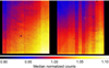 |
Fig. B.1. Dark-subtracted and bad-pixel-filtered flat-field frame in the Ks-band showing the total-intensity-dependent gradient in the left and right images on the detector. |
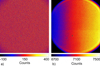 |
Fig. B.2. Double-difference images of the unpolarized source (a) and polarized source measurements (b) in the Ks-band showing that the double difference completely removes the total-intensity-dependent gradient, but does not remove the polarization-dependent-gradient. |
In the polarized source measurements, the double difference removes the total-intensity-dependent gradient, but a polarization-dependent-gradient remains (see Fig. B.2b). This gradient is different in strength and orientation for each exposure and therefore seems to depend on the orientation of the HWP and/or derotator. Because the HWP is close to a focal plane, a likely cause of the polarization-dependent-gradient is that the retardance of the HWP varies over the surface of the HWP. The gradient is not visible in the unpolarized source measurements, because the incident light is only very weakly polarized in that case.
Appendix C: Graphs of model fits of internal calibration measurements
Figure C.1 shows the ideal, measured, and fitted normalized Stokes parameters of the polarized source measurements in the H-band as a function of HWP and derotator angle, including the residuals of fit. The ideal curves are computed with the HWP and derotator retardances equal to 180°, no angle offsets and the diattenuation of the polarizers equal to 1. The measured and fitted normalized Stokes parameters of the unpolarized source measurements in the H-band are displayed in Figs. C.2 (normal double difference) and C.3 (modified double difference with the derotator angles, rather than the HWP angles, differing 45° between the two exposures). These figures also show the corresponding residuals of fit. The ideal curves (completely unpolarized light incident on the HWP, the diattenuations of the HWP, derotator, and polarizers equal to 1, and no angle offsets) coincide with the x-axes of the graphs and are therefore not shown.
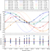 |
Fig. C.1. Ideal, measured, and fitted normalized Stokes parameters of the polarized source measurements in the H-band as a function of HWP and derotator angle. The legend only shows the |


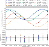 |
Fig. C.2. Measured and fitted normalized Stokes parameters of the unpolarized source measurements in the H-band (normal double difference with the two HWP angles differing 45°) as a function of HWP and derotator angle. The legend only shows the |


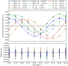 |
Fig. C.3. Measured and fitted normalized Stokes parameters of the unpolarized source measurements in the H-band (modified double difference with the two derotator angles, rather than the HWP angles, differing 45°) as a function of derotator and HWP angle. The legend only shows the |


Appendix D: Determination of normalized Stokes parameters and graphs of model fits of unpolarized star observations
The normalized Stokes parameters of the observations of the unpolarized stars are determined from apertures in the Q-, U-, IQ-, and IU-images. For the data of HD 217343 (2018), we compute the signal in these images as the mean in an aperture minus the median of the background signal in a concentric annulus. We then calculate the normalized Stokes parameter q or u by dividing the signal from the Q- or U-image by that from the corresponding IQ- or IU-image according to Eq. (10). The radii of the apertures used are determined from plots of the normalized Stokes parameters as a function of aperture radius (see Fig. D.1). In all filters an aperture radius of 220 pixels is used, because at this radius the curves have approached a constant value. The annulus to compute the background signal from starts at the outer radius of the aperture and has a width of 40 pixels.
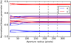 |
Fig. D.1. Normalized Stokes parameters q and u as a function of aperture radius for the observations of the unpolarized star HD 217343 (2018) in the H-band. The central and outer dashed lines indicate the radii of the apertures from which the normalized Stokes parameters and their error bars (see Figs. 9 and D.5) have been determined, respectively. |
For the data of HD 176425 (2016) we use the same method to compute the normalized Stokes parameters, but we do not subtract the background signal. This is because almost the complete image is filled with signal from the star and therefore there is no location to accurately determine the background signal from. In the Y-, J-, and H-band, where we use an aperture radius of
200 pixels, this is no problem because the background signal is very small.
In the Ks-band however (see Fig. D.2), the curves of q and u versus aperture radius do not approach a constant value, but decrease with increasing aperture radii due to the much stronger background signal that most likely originates from thermal emission of the UT and SPHERE’s uncooled optics upstream from IRDIS. Because the intensity of the star’s point spread function (PSF) decreases with increasing distance from the center, the thermal background becomes more prominent for larger aperture radii. Although the thermal background is removed after computing the double difference (Q- and U-images), it is not removed after computing the double sum (IQ- and IU-images), and therefore the normalized Stokes parameters decrease with increasing aperture radius. An aperture radius of 125 pixels is selected for the measurements in the Ks-band, because at this radius: (1) the curves of the other filters start to approach a constant value, (2) the thermal background starts to become visible in the raw frames, and (3) the determined diattenuations of the UT and M4 are in line with expectations based on the determined diattenuations in the other filters and their deviation from the analytical values (see Fig. 10).
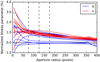 |
Fig. D.2. Normalized Stokes parameters q and u as a function of aperture radius for the observations of the unpolarized standard star HD 176425 (2016) in the Ks-band. The central and outer dashed lines indicate the radii of the apertures from which the normalized Stokes parameters and their error bars (see Figs. 8 and D.4) have been determined, respectively. |
Figures D.3 and D.4 show the analytical, measured, and fitted normalized Stokes parameters q and u of the observations of HD 176425 (2016) as a function of telescope altitude angle in the H- and Ks-band, respectively. Figure D.5 shows the same graph for the observations of HD 217343 (2018) in the H-band. The residuals of fit are also included in these figures. The analytical curves are computed from the Fresnel equations using the complex refractive index of aluminum. The error bars are calculated as half the difference between the normalized Stokes parameters determined from apertures with radii 50 pixels larger and smaller than the radius of the aperture used to calculate q and u used for determining the diattenuations (see Figs. D.1 and D.2). The error bars show the uncertainty in the normalized Stokes parameters due to the dependency of the measured values on the chosen aperture radius. These uncertainties are small for all measurement except those of HD 176425 (2016) in the Ks-band because the thermal background could not be subtracted. Finally, because we did not keep the derotator fixed with its plane of incidence horizontal for the observations of HD 217343 (2018), crosstalk from the derotator causes the shape of the curves in Fig. D.5 to be different from those of Figs. D.3 and D.4.
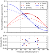 |
Fig. D.3. Analytical (aluminum), measured (including error bars), and fitted normalized Stokes parameters q and u as a function of telescope altitude angle for the observations of the unpolarized standard star HD 176425 (2016) in the H-band. For science observations the telescope altitude angle is restricted to 30° ≤a ≤ 87°. |
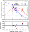 |
Fig. D.4. Analytical (aluminum), measured (including error bars), and fitted normalized Stokes parameters q and u as a function of telescope altitude angle for the observations of the unpolarized standard star HD 176425 (2016) in the Ks-band. For science observations the telescope altitude angle is restricted to 30° ≤a ≤ 87°. |
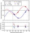 |
Fig. D.5. Analytical (aluminum), measured (including error bars), and fitted normalized Stokes parameters q and u as a function of telescope altitude angle for the observations of the unpolarized star HD 217343 (2018) in the H-band. For science observations the telescope altitude angle is restricted to 30° ≤a ≤ 87°. |
Appendix E: Calculation of accuracies of fit and uncertainties in determined parameters
To estimate the polarimetric accuracy of the instrument model, we calculate for each broadband filter the accuracies of fitting the model parameters to the calibration data. We compute these accuracies of fit as the corrected sample standard deviation of the residuals sres:
 (E.1)
(E.1)
with ri the residuals of fit, n the number data points, and k the number of parameters determined from the data set. The accuracies of fit are calculated separately for the polarized source measurements, the unpolarized source measurements, and the two observations of unpolarized stars (denoted srel, sunpol, and sstar, respectively, in Sect. 7). The results are shown in Table E.1.
Accuracies of fit of the polarized source measurements, the unpolarized source measurements, and the observations of the unpolarized stars HD 176425 (2016) and HD 217343 (2018) in the Y-, J-, H-, and Ks-band.
To compute the uncertainties of the determined model parameters, we approximate the covariance matrix of the model parameters Σ as:
 (E.2)
(E.2)
where J is the Jacobian matrix:
 (E.3)
(E.3)
with β1 to βm the m determined model parameters and x1 to xn the model functions describing the n measurements (Eq. (10) with the model equations and the parallactic, altitude, derotator, and HWP angles of the measurements substituted). The matrix τ has dimensions m × m and contains on its diagonal for each model parameter the accuracy of fit (sres) of the measurements from which that parameter is determined (see Table E.1). For example, the diagonal element of τ corresponding to the model parameter 𝛥der in the H-band is equal to sres of the polarized source measurements in the same filter. Finally, we compute the 1σ-errors (1 times the standard deviation) of the model parameters as the square root of the diagonal elements of Σ, and list them behind the ±-signs in Tables 1 and 2.
By taking the diagonal values of Σ as the uncertainties of the parameters, it is assumed that the parameter values are not correlated. However, in reality all the parameters are weakly correlated, in particular because the offset angles δHWP, δder, and δcal are determined from the complete set of polarized source measurements. In addition, the uncertainties of the parameters are computed using a linear approximation through the Jacobian. Therefore the uncertainties should be considered first order estimates only.
All Tables
Determined parameters and their errors of the part of the model describing the instrument downstream of M4 in the Y-, J-, H-, and Ks-band.
Determined diattenuations with their errors and computed retardances of the part of the model describing the telescope and M4 in the Y-, J-, H-, and Ks-band.
Polarimetric accuracy of measuring the degree and angle of linear polarization of a 1% polarized substellar companion and a 30% polarized circumstellar disk in the Y-, J-, H-, and Ks-band before the re-aluminization of M1 and M3.
Accuracies of fit of the polarized source measurements, the unpolarized source measurements, and the observations of the unpolarized stars HD 176425 (2016) and HD 217343 (2018) in the Y-, J-, H-, and Ks-band.
All Figures
|
Fig. 1. Reference frame for the definition of the Stokes parameters describing the oscillation direction of the electric field within a beam of light. The propagation direction of the light beam is out of the paper, toward the reader. Positive and negative Stokes Q are oriented along the vertical (+Q) and horizontal (−Q) axes, respectively. Looking into the beam of light, positive Stokes U (+U) is oriented 45° counterclockwise from positive Stokes Q and positive Stokes V (+V) is defined as clockwise rotation. The angle of linear polarization AoLP and the rotation angle θ of an optical component used in the rotation Mueller matrix (see Eqs. (15) and (16)) are defined counterclockwise when looking into the beam of light. |
| In the text | |
|
Fig. 2. Overview of the optical path of the complete optical system, i.e., the Unit Telescope (UT) and SPHERE/IRDIS, showing only the components relevant for polarimetric measurements (image adapted from Fig. 2 of Paper I). The names of the (groups of) components are indicated in boldface. The black circular arrows indicate the astronomical target’s parallactic angle p, the telescope’s rotation with the altitude angle a, the offset angle of the calibration polarizer δcal, and the rotation of the HWP and image derotator with the angles θHWP + δHWP and θder + δder, respectively. Also shown are the parameters describing the instrumental polarization effects of the (groups of) components: the component diattenuations ϵ, retardances 𝛥 and the polarizer diattenuation d. The Stokes vectors Sin, SHWP, Sdet, L, Sdet, R and |
| In the text | |
|
Fig. 3. Measured and fitted polarimetric efficiency of the instrument downstream of M4 as a function of HWP and derotator angle in the H-band. The legend only shows the |
| In the text | |
|
Fig. 4. Measured and fitted offset of the angle of linear polarization induced by the instrument downstream of M4 as a function of HWP and derotator angle in the H-band. The legend only shows the |
| In the text | |
|
Fig. 5. Measured and fitted polarimetric efficiency of the instrument downstream of M4 with |
| In the text | |
|
Fig. 6. Measured and fitted offset of angle of linear polarization induced by the instrument downstream of M4 with |
| In the text | |
|
Fig. 7. HWP retardance as a function of wavelength as specified by the manufacturer2 compared to the determined HWP retardance (𝛥HWP) in the Y-, J-, H-, and Ks-band. |
| In the text | |
|
Fig. 8. Analytical (aluminum), measured (including error bars), and fitted instrumental polarization (IP) of the telescope and M4 as a function of telescope altitude angle in the Y-, J-, H-, and Ks-band from the measurements of HD 176425 taken in 2016 before the re-aluminization of M1 and M3. For science observations the telescope altitude angle is restricted to 30° ≤a ≤ 87°. |
| In the text | |
|
Fig. 9. Analytical (aluminum), measured (including error bars) and fitted instrumental polarization (IP) of the telescope and M4 as a function of telescope altitude angle in the Y-, J-, H-, and Ks-band from the measurements of HD 217343 taken in 2018 after the re-aluminization of M1 and M3. For science observations the telescope altitude angle is restricted to 30° ≤a ≤ 87°. |
| In the text | |
|
Fig. 10. Instrumental polarization (IP) of the UT and M4 separately, as determined from the various measurements, versus central wavelength of the Y-, J-, H-, and Ks-band. The curves show the IP of the UT and M4 from the observations of the unpolarized stars HD 176425 (on-sky 2016) and HD 217343 (on-sky 2018), the IP of M4 from the unpolarized source measurements and the IP of the UT and M4 computed from the Fresnel equations (aluminum analytical). |
| In the text | |
|
Fig. 11. Flow diagram showing the steps to construct the incident |
| In the text | |
|
Fig. 12. Effect of the data-reduction steps of our correction method on the Stokes U-images of the first and last (30th) HWP cycle of the observations of the circumstellar disk of T Cha. |
| In the text | |
|
Fig. 13. Polarized intensity and angle of linear polarization of the circumstellar disk of T Cha after applying the correction method. The white lines indicating the angle of linear polarization have arbitrary length and are only shown where the polarized intensity is higher than 50 counts. |
| In the text | |
|
Fig. 14. Final azimuthal Stokes Qϕ- and Uϕ-images of the circumstellar disk of T Cha after applying our correction method compared to the images generated with the conventional IP-subtraction method from Canovas et al. (2011). Positive Qϕ indicates linear polarization in the azimuthal direction and Uϕ shows the linear polarization at ±45° from this direction. The color scales of the top and bottom row are different, i.e., the signals in Qϕ are almost 10 times larger than the signals in Uϕ. |
| In the text | |
|
Fig. 15. Normalized Stokes parameters of the measured stellar polarization of T Cha as function of HWP cycle after applying our correction method. |
| In the text | |
|
Fig. B.1. Dark-subtracted and bad-pixel-filtered flat-field frame in the Ks-band showing the total-intensity-dependent gradient in the left and right images on the detector. |
| In the text | |
|
Fig. B.2. Double-difference images of the unpolarized source (a) and polarized source measurements (b) in the Ks-band showing that the double difference completely removes the total-intensity-dependent gradient, but does not remove the polarization-dependent-gradient. |
| In the text | |
|
Fig. C.1. Ideal, measured, and fitted normalized Stokes parameters of the polarized source measurements in the H-band as a function of HWP and derotator angle. The legend only shows the |
| In the text | |
|
Fig. C.2. Measured and fitted normalized Stokes parameters of the unpolarized source measurements in the H-band (normal double difference with the two HWP angles differing 45°) as a function of HWP and derotator angle. The legend only shows the |
| In the text | |
|
Fig. C.3. Measured and fitted normalized Stokes parameters of the unpolarized source measurements in the H-band (modified double difference with the two derotator angles, rather than the HWP angles, differing 45°) as a function of derotator and HWP angle. The legend only shows the |
| In the text | |
|
Fig. D.1. Normalized Stokes parameters q and u as a function of aperture radius for the observations of the unpolarized star HD 217343 (2018) in the H-band. The central and outer dashed lines indicate the radii of the apertures from which the normalized Stokes parameters and their error bars (see Figs. 9 and D.5) have been determined, respectively. |
| In the text | |
|
Fig. D.2. Normalized Stokes parameters q and u as a function of aperture radius for the observations of the unpolarized standard star HD 176425 (2016) in the Ks-band. The central and outer dashed lines indicate the radii of the apertures from which the normalized Stokes parameters and their error bars (see Figs. 8 and D.4) have been determined, respectively. |
| In the text | |
|
Fig. D.3. Analytical (aluminum), measured (including error bars), and fitted normalized Stokes parameters q and u as a function of telescope altitude angle for the observations of the unpolarized standard star HD 176425 (2016) in the H-band. For science observations the telescope altitude angle is restricted to 30° ≤a ≤ 87°. |
| In the text | |
|
Fig. D.4. Analytical (aluminum), measured (including error bars), and fitted normalized Stokes parameters q and u as a function of telescope altitude angle for the observations of the unpolarized standard star HD 176425 (2016) in the Ks-band. For science observations the telescope altitude angle is restricted to 30° ≤a ≤ 87°. |
| In the text | |
|
Fig. D.5. Analytical (aluminum), measured (including error bars), and fitted normalized Stokes parameters q and u as a function of telescope altitude angle for the observations of the unpolarized star HD 217343 (2018) in the H-band. For science observations the telescope altitude angle is restricted to 30° ≤a ≤ 87°. |
| In the text | |
Current usage metrics show cumulative count of Article Views (full-text article views including HTML views, PDF and ePub downloads, according to the available data) and Abstracts Views on Vision4Press platform.
Data correspond to usage on the plateform after 2015. The current usage metrics is available 48-96 hours after online publication and is updated daily on week days.
Initial download of the metrics may take a while.