| Issue |
A&A
Volume 633, January 2020
|
|
|---|---|---|
| Article Number | A21 | |
| Number of page(s) | 15 | |
| Section | Planets and planetary systems | |
| DOI | https://doi.org/10.1051/0004-6361/201834945 | |
| Published online | 24 December 2019 | |
Global axisymmetric simulations of photoevaporation and magnetically driven protoplanetary disk winds
1
Institute for Theoretical Astrophysics, Zentrum für Astronomie, Heidelberg University,
Albert Ueberle Str. 2,
69120
Heidelberg,
Germany
e-mail: This email address is being protected from spambots. You need JavaScript enabled to view it.
2
Max-Planck-Institut für Astronomie,
Königstuhl 17,
69117
Heidelberg,
Germany
Received:
21
December
2018
Accepted:
8
November
2019
Abstract
Context. Photoevaporation and magnetically driven winds are two independent mechanisms that remove mass from protoplanetary disks. In addition to accretion, the effect of these two principles acting concurrently could be significant, and the transition between them has not yet been extensively studied and quantified.
Aims. In order to contribute to the understanding of disk winds, we present the phenomena emerging in the framework of two-dimensional axisymmetric, nonideal magnetohydrodynamic simulations including extreme-ultraviolet (EUV) and X-ray driven photoevaporation. Of particular interest are the examination of the transition region between photoevaporation and magnetically driven wind, the possibility of emerging magnetocentrifugal wind effects, and the morphology of the wind itself, which depends on the strength of the magnetic field.
Methods. We used the PLUTO code in a two-dimensional axisymmetric configuration with additional treatment of EUV and X-ray heating and dynamic ohmic diffusion based on a semi-analytical chemical model.
Results. We determine that the transition between the two outflow types occurs for values of the initial plasma beta β ≥ 107, while magnetically driven winds generally outperform photoevaporation for stronger fields. In our simulations we observe irregular and asymmetric outflows for stronger magnetic fields. In the weak-field regime, the photoevaporation rates are slightly lowered by perturbations of the gas density in the inner regions of the disk. Overall, our results predict a wind with a lever arm smaller than 1.5, consistent with a hot magnetothermal wind. Stronger accretion flows are present for values of β < 107.
Key words: protoplanetary disks / accretion, accretion disks / hydrodynamics / magnetic fields / magnetohydrodynamics (MHD)
© ESO 2019
1 Introduction
Protoplanetary disks have an observed lifetime that ranges from 2 to 6 Myr (Haisch et al. 2001; Mamajek et al. 2004; Ribas et al. 2015). The physical processes that constrain and shape the evolution of these disks are highly debated.
One possible explanation for the limited lifetime is the phenomenon of accretion. In the study of accretion disks around black holes, Shakura & Sunyaev (1973) invoked the scenario that an α viscosity based on underlying turbulent effects drives the accretion flow. The concept can be applied to circumstellar disks, where several instabilities have been postulated over the last decades.
When the disk mass reaches a significant fraction of the stellar mass, gravitational instability (GI) (Toomre 1964) can operate, leading to spirals, fragmentation, and accretion flows. The nonlinear evolution of GI leads to a gravoturbulent state, depending on the balance of shock heating, compression heating, and cooling (Durisen et al. 2007), and it can be incorporated into α disk models (Lin & Pringle 1987). The critical cooling timescale for self-gravitating turbulence has been studied numerically by Lodato & Rice (2004, 2005) and Paardekooper et al. (2011), for example.
A prominent mechanism that can explain turbulence-driven accretion is magnetorotational instability (MRI; Balbus & Hawley 1991), which involves a well-ionized medium and a weak magnetic field embedded in a differentially rotating disk. Numerous studies on the convergence and influence of nonideal magnetohydrodynamic (MHD) effects in the framework of local shearing box simulations have been published, for instance, Fromang & Papaloizou (2007), Bai (2011) and Hirose & Turner (2011). Global simulations including ohmic diffusion were carried out, for example, by Dzyurkevich et al. (2010) and Flock et al. (2011).
Because the deeper layers of the disk are weakly ionized (Igea & Glassgold 1999), ohmic diffusion dominates in the mid-plane, inhibiting MRI activity and thus creating a “dead zone” (Gammie 1996). Its structure has been studied in global simulations by Dzyurkevich et al. (2013). In addition to MRI, hydrodynamic instabilities can potentially operate in the dead zone. Examples are vertical shear instability (VSI; Nelson et al. 2013), Rossby-wave instability (RWI; Lovelace et al. 1999), global baroclinic instability (Klahr & Bodenheimer 2003), and convective overstability (Klahr & Hubbard 2014).
As a different concept, a disk threaded by a large scale, an open magnetic field can develop magnetically (or magnetocentrifugally) driven winds that lead to angular momentum transfer and consequently cause accretion flows. A semi-analytical description of this concept has first been presented in the seminal paper of Blandford & Payne (1982). In order to allow for stationary solutions, turbulent diffusivity has been assumed in the mid-plane of the disk (Wardle & Koenigl 1993; Ferreira & Pelletier 1993, 1995). These winds present a viable alternative solution to the α disk model.
Casse & Keppens (2002) presented the first global simulations in which a jet was launched from a resistive disk. Similar simulations on a longer timescale have been reported by Zanni et al. (2007) with β = 1 in the mid-plane and extended ranges of viscosity and resistivity. Tzeferacos et al. (2009) observed unsteady winds up to β ≈ 500. Sheikhnezami et al. (2012) studied the effect of the magnitude and distribution of the magnetic diffusivity on the mass loading of the jet, and Fendt & Sheikhnezami (2013) focused on the symmetry of bipolar outflows.
Stepanovs & Fendt (2014, 2016) found the jet characteristics to be correlated to the disk magnetization and identified a transition between jets driven by magnetocentrifugal forces and magnetic pressure at β ≈ 100. Furthermore, the disk magnetization can change substantially throughout the dynamical evolution of the outflow and the disk.
Gressel et al. (2015) simulated global magnetically driven disk winds for weaker fields around β = 105 including ohmic and ambipolar diffusion. Béthune et al. (2017) included ohmic diffusion, ambipolar diffusion, and the Hall effect in magnetothermal wind simulations that included heating of the upper layers of the disk. The authors found asymmetric winds in some cases. Bai (2017) conducted a study that also included all three nonideal MHD effects with a comprehensive microphysical treatment.
In the framework of local shearing box simulations, Suzuki & Inutsuka (2009) found that a wind was launched from MRI turbulent layers at about two disk scale heights where the plasma beta β = 8πP∕B2 (the ratio of thermal to magnetic pressure) reaches unity, assuming β to be 106 in the mid-plane. A flow like this may create an inner hole in the disk (Suzuki et al. 2010).
In local simulations of Bai & Stone (2013a), the wind mass-loss rate was observed to be proportional to 1∕β up to a mid plane β = 100. Bai & Stone (2013b) stated that the MRI is suppressed at 1 au and that for β = 105 a wind is launched at four disk scale heights. However, it was pointed out that the outflow rate may be sensitive to the applied resolution in local simulations (Fromang et al. 2013).
As an alternative to magnetically driven winds, outflows can be solely thermally driven through ionizing radiation from the central star or external sources. Possible types of radiation causing these photoevaporative winds are extreme-ultraviolet (EUV) radiation (Hollenbach et al. 1994), far-ultraviolet (FUV) radiation (Adams et al. 2004; Gorti & Hollenbach 2004, 2009) and X-ray radiation (Ercolano et al. 2009; Owen et al. 2010, 2012; Picogna et al. 2019). Photoevaporation does not drive accretion flows, therefore these winds merely act as a mass sink for the underlying disk.
The interplay between the two mechanisms of magnetically driven winds and photoevaporation has not been subject of detailed study in the past. Only recently, a combination of these concepts has been presented by Wang et al. (2019), involving global 2.5D magnetohydrodynamic simulations. In their model the simplified radiative transfer is evolved during each hydro step.
In this paper we use the recent photoevaporation model by Picogna et al. (2019) with a precomputed temperature prescription originating from detailed radiative transfer and photoionization calculations including EUV and X-ray radiation. We extend the fiducial model by applying a large-scale magnetic field. Thereby, we can study the wind rates depending on the magnetic field strength in order to identify the transition region of magnetically driven winds and photoevaporation.
The paper is organized as follows: in Sect. 2 the general concept and theory of the two disk-wind mechanisms are outlined. Section 3 introduces the numerical model we used in our simulations, that is, the EUV and X-ray heating, ionization model, and disk properties. In Sect. 4 we present the main results of our study, including wind flow, transition region, magnetic field evolution, and accretion flows. In Sects. 5 and 6 these results are discussed and summarized.
2 Theory
2.1 Magnetically driven outflows
In general, magnetically driven outflows involve mass loss in the form of winds that are caused by a sufficiently ionized rotating disk threaded by a magnetic field. The wind-launching mechanism depends on the magnetic field strength, and the launching mechanism can be divided into two regimes with either strong or weak magnetic fields. These two regimes are magnetocentrifugal winds with strong magnetic fields and with winds that are solely driven by the magnetic pressure gradient if the magnetic field is weak. In between these extremes, a smooth transition exists at intermediate field strengths (Bai 2016).
In the strong-field limit, the magnetic field lines rotate approximately rigidly up to the Alfvén surface, andthe wind is magnetocentrifugally accelerated (Blandford & Payne 1982; Pudritz & Norman 1983). The condition for this wind to occur is that the magnetic field is inclined by less than 60° to the disk. In this picture, the accelerated gas can be pictured like a string of pearls (the “string” being magnetic field lines). The inclination condition can be relaxed to 70° when a hot wind is assumed (Pelletier & Pudritz 1992).
Because we assume corotating field lines (i.e., the angular frequency along the field lines is approximately equal to the Keplerianangular frequency at the foot point of the wind), the gas parcels carry away angular momentum from the foot point at the disk. This results in an inflow of gas.
Accretion and wind-loss rates can be connected in the framework of magnetocentrifugally driven winds. The wind extracts a specific angular momentum of  when it corotates up to the Alfvén radius rA starting from the foot point r0. The relation between the (cumulative) wind mass-loss rate Ṁw and the accretion rate Ṁacc can be derived as (Ferreira & Pelletier 1995; Bai et al. 2016)
 (1)
(1)
with the so-called magnetic lever arm λ. The condition λ ≥ 1.5 holds for cold MHD winds, and a smaller lever arm is possible when a warm or hot magnetothermal wind is assumed (Bai 2016).
Throughout this paper the cylindrical radius is denoted by r and the vertical cylindrical coordinate is represented by z. The spherical radius R is thus given by
 (2)
(2)
In the strong magnetic field limit the outflow can collimate to a jet (Casse & Keppens 2002). With decreasing magnetic field strengths, the wind flows in a wider angle and becomes increasingly driven by the magnetic pressure gradient, which is in contrast to the centrifugal acceleration with a strong magnetic field. In the context of this “magnetic tower wind” (Lynden-Bell 1996, 2003), the toroidal magnetic field is dominant and the Alfvén surface lies close to the wind-launching front. Consequently, the angular momentum transport is small and the accretion rate decreases in the disk, which leaves the wind as the dominant cause for mass loss. Moreover, in the transition from strong to weak magnetic fields, the wind topology changes from a jet-like structure to a more unsteady, episodic wind (Sheikhnezami et al. 2012).
2.2 Photoevaporation and X-ray heating
The fundamental idea of photoevaporation is that high-energy radiation ionizes parts of the circumstellar disk and thereby heats the topmost disk layers. These hot layers subsequently expand and produce a pressure-driven transonic wind, similar to a Parker wind. The mechanism can be divided into external photoevaporation, where the ionizing radiation originates from external source (e.g., O stars) and internal photoevaporation, where the central star provides the driving radiation. We consider only the latter here.
The energy of the incoming radiation can be categorized into three regimes: FUV (6–13.6 eV), EUV (13.6–100 eV), and X-ray (0.1–100 keV) radiation. Typical mass-loss rates expected from photoevaporation are about 3 × 10⁻⁸ M⊙ yr−1 (Gorti & Hollenbach 2009).
In models of EUV-driven photoevaporation, the photon flux ionizes hydrogen atoms in the upper atmosphere layers of theprotoplanetary disk. Thereby, the created diffuse recombination radiation heats up the outer regions of the disk (Hollenbach et al. 1994; Clarke et al. 2001; Font et al. 2004), leading to mass-loss rates of ≈ 4 ×10⁻¹⁰ M⊙ yr−1. A characteristic length scale of these systems is the so-called gravitational radius,
 (3)
(3)
where cs is the isothermal sound speed, G is the gravitational constant, and M* is the stellar mass. With ionization temperatures of ≈104 K and assuming a solar mass star, Rg is ≈ 9 au. However, more detailed studies (Adams et al. 2004; Font et al. 2004) have shown that the sharp division, induced by the gravitational radius, is in fact a more diffuse boundary, situated at roughly 0.1–0.2 Rg (critical radius) (Dullemond et al. 2007). In the long-term evolution of photoevaporation in combination with viscous evolution, a two-timescale behavior emerges. This creates a gap at Rg when the local accretion rate is comparable to the wind mass-loss rate. Then, the inner disk quickly accretes onto the star within about 105 yr (Clarke et al. 2001).
With an inner hole, direct illumination of the outer part leads to thermal sweeping. This clears the remaining disk in an inside-out fashion (Owen et al. 2012; Haworth et al. 2016).
X-ray photons are able to penetrate deeper into the disk atmosphere than EUV radiation (column densities of ≈ 1022 cm−2 Ercolano et al. 2009; Owen et al. 2010). Owen et al. (2010) argued that X-ray driven photoevaporation leads to significantly higher mass-loss rates than the EUV case. Models of Owen et al. (2010, 2012) indicate a mass-loss rate of 1.4 × 10⁻⁸ M⊙ yr−1 for solar-like stars, involving the concept of an ionization parameter,
 (4)
(4)
where Lx denotes the luminosity of the central X-ray radiation source and n the local number density of the gas. By computing a relation between ξ and the local gas temperature, tabulated values can be interpolated locally during the hydrodynamical simulation because in-place calculations of the temperatures would be computationally prohibitive. The main assumption here is that we are in the optically thin regime and hence X-ray attenuation can be neglected up to the limiting column density. Defining a gravitational radius in this case is less useful because the gas temperatures depend on the density, and the heated layers cannot be assumed to be isothermal.
Far-ultraviolet radiation can heat the ambient medium by photoelectric heating of grains as well as by vibrational excitation and collisional relaxation of H2 molecules (Hollenbach & Tielens 1999). Gorti & Hollenbach (2009) found an FUV-dominated mass-loss rate of ≈ 3 ×10⁻⁸ M⊙ yr−1 at a distance range of 100 to 200 au, which is comparable to X-ray photoevaporation. However, the temperatures in FUV-heated regions are sensitive to the uncertain abundance of polycyclic aromatic hydrocarbons (PAHs; Geers et al. 2009). Because of these drawbacks and the chemical complexity, we restrict our model to EUV and X-ray dominated heating.
3 Numerical model
All simulations of this paper are two-dimensional axisymmetric, including the toroidal velocity and magnetic field component (i.e., 2.5 dimensional). They were carried out with the PLUTO code (version 4.3) (Mignone et al. 2007, 2012), which allows solving the MHD equations on a spherical grid, including ohmic resistivity. Throughout this section, we present the basis of the numerical model, that is, the X-ray and EUV heating approach, disk structure, magnetic field, and dynamic treatment of ohmic diffusion.
3.1 MHD equations
Relevant equations are the conservation of mass,
 (5)
(5)
the conservation of momentum,
 (6)
(6)
the energy equation,
![Mathematical equation: \begin{eqnarray*}&& \hspace*{-6pt}\frac{ \partial e}{\partial t} + \nabla \cdot \left[ \bm{v} \left(\!e + P + \frac{B^2}{8 \pi}\!\right) - \frac{1}{4 \pi} (\bm{v} \cdot \bm{B}) \bm{B} + \left( \eta \cdot \bm{J} \right) \times \bm{B} \right] \nonumber \\[2pt] && \hspace*{-4pt}\quad = - \rho (\nabla \Phi) \cdot \bm{v} ,\end{eqnarray*}](/articles/aa/full_html/2020/01/aa34945-18/aa34945-18-eq8.png) (7)
(7)
and the induction equation,
 (8)
(8)
where P is the thermal gas pressure, ρ the gas density, B the magnetic flux density vector, J the electric current density vector, η the ohmic diffusion coefficient, v the gas velocity vector, and  the gravitational potential.
To update the cells, the HLLD Riemann solver (Miyoshi & Kusano 2005) was used. To ensure the condition ∇ ⋅ B = 0, the divergence cleaning method (Dedner et al. 2002) was applied. All simulations were evolved with an adiabatic equation of state, using an isentropic exponent of κ = 5∕3.
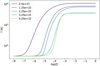 |
Fig. 1 Ionization parameter–temperature relation based on the data in Picogna et al. (2019). |
3.2 Diagnostics
The relativestrength of the magnetic field can be expressed with the dimensionless plasma parameter β:
 (9)
(9)
which is the ratio of thermal pressure over magnetic pressure.
In order to evaluate the nonideal MHD effects (ohmic diffusion) on possible MRI activity, the notion of an ohmic Elsasser number ΛΩ (Turner et al. 2007) is useful:
 (10)
(10)
Here vA is the Alfvén velocity and η the ohmic diffusion coefficient. Generally, MRI is considered to be suppressed for ΛΩ ≲ 1.
The integrated mass-loss rate caused by the wind is computed by the expression
 (11)
(11)
and the disk region is excluded from the range in θ. Here, vR denotes the radial velocity component of the flow.
3.3 EUVand X-ray heating
Following the approach of Owen et al. (2010, 2012, 2013), X-ray heating was provided by using a fitted ionization parameter - temperature relation T = f(ξ), taken from Picogna et al. (2019). In addition to the previously studied models, the temperature curves depend on the local column density, as shown in Fig. 1. Knowing the dependence of the temperature on the local variables, we traced rays from the inner simulation boundary radially outward up to column densities of 5 × 1022 cm−2. Within this range, the temperatures were set corresponding to the locally computed ionization parameter using the fitted relation f(ξ). With intermediate column densities, the temperature is linearly interpolated.
The temperature adjustment was only invoked when the temperature computed by the ionization model was higher than the local gas temperature. No relaxation time was applied. The regions that were unaffected by the photoevaporation heating were treated according to the energy equation (Eq. (7)). The resulting pressure in the simulations depends on the mean molecular weight μ. Similarly to the models of Owen et al. (2010), we set it to μ = 1.37125, which is suitable for ionized gas, including atomic hydrogen.
The implementation, depending on the column density, provides a more accurate treatment of the regime between optically thin and thick gas, where X-ray attenuation becomes significant. The temperature parameterization was computed by 3D photoionization and radiative transfer calculations.Thus the diffuse, secondary radiation field was taken into account. Essentially, the same initial parameters for the luminosity and the photon energy can be used to assemble a consistent model regarding the ionization rate for the ohmic diffusion coefficients (cf. Sect. 3.4.4).
3.4 Disk model
3.4.1 Initial density structure
The initial density structure we used in the simulations can be formulated as
 (12)
(12)
where Σ(r) is the vertically integrated column density. The scaling with the cylindrical radius r corresponds to a column density gradient of p = 1. When we assume an initial disk mass of ≈0.05 M⊙, the value of Σ(r = 1 au) is equal to ≈711 g cm−2.
For the initial thermal structure, the prescription from Hayashi (1981) was used,
 (13)
(13)
which corresponds to a temperature gradient of q = 1∕2 and causes the disk to be flared (H∕r not constant with radius). The dust temperature was assumed to be equal to the gas temperature in our model.
With the assumption of hydrostatic equilibrium and an isothermal, vertically stratified disk atmosphere, the density can be written as
![Mathematical equation: \begin{equation*}\rho(r, z) = \rho_{\textrm{mid}} \, \textrm{exp} \left[ \frac{r^2}{H^2} \left( \frac{r}{R} - 1 \right) \right] ,\end{equation*}](/articles/aa/full_html/2020/01/aa34945-18/aa34945-18-eq16.png) (14)
(14)
where H = cs∕ΩK is the pressure scale height and ρmid is the mid-plane density at z = 0.
For z ≪ r, Eq. (14) reduces to the conventional form ρmid exp(−z2∕(2H2)). However, Eq. (14) was used in our simulations because the disk has a significant vertical extent. The isothermal sound speed is given by  . We chose the mean molecular weight to be μ = 1.37125, equal to the weight of the X-ray heated gas.
The density in the mid-plane is calculated with the column density by  . In a more general setting with surface density scaling as Σ ∝ rp and temperature scaling as Tmid ∝ rq, we find that ρmid scales proportionally to r−p+(3−q)∕2 (because H ∝ r(3−q)∕2).
In protoplanetary disks, the toroidal velocity has to be lower than Keplerian because of the additional pressure force, which points outward. When we take vertical variations into account, the velocity in azimuthal direction can be defined as (using Eq. (9) of Bai 2017)
![Mathematical equation: \begin{equation*} v_{\phi}(r, R) = r \Omega_K \left[ 1 - (2p + (3-q)/2) \frac{H^2}{r^2} + q \frac{r - R}{R} \right] .\end{equation*}](/articles/aa/full_html/2020/01/aa34945-18/aa34945-18-eq19.png) (15)
(15)
By taking these vertical corrections into account, an initially more stable disk configuration can be achieved in the simulations. In order to verify the stability, the setup was tested without photoevaporation effects and magnetic fields.
3.4.2 Coronal gas structure
The whole disk in the simulations is surrounded by a hydrostatically stable corona, consisting of gas whose density is much lower than that of the disk. Its purpose is to define a reasonable density floor value for numerical stability. When the mass of the sphere itself is neglected, the hydrostatic balance can be written as
 (16)
(16)
where ri is the radius at the inner boundary of the simulation domain and γ is the adiabatic index (γ = 5∕3 in the simulations). The density at the inner boundary ρc0(ri) is related to the disk density in the mid-plane and ri with the density contrast δ = ρc0(ri)∕ρmid(ri). The definition of the corona is the same as in Sheikhnezami et al. (2012). The pressure can be conveniently scaled with the Keplerian velocity at the inner boundary,
 (17)
(17)
In the simulations performed here, the upper limit of this density contrast was heavily constrained by the photoevaporation because the coronal gas should allow rays to traverse the whole simulation domain, without being absorbed completely or affected significantly. We therefore set the density contrast to δ = 10−8. The corona is mostly blown away by the emerging wind, but we find the solution to be numerically more stable with this prescription and its application as a density floor at every integration step. By updating the density to the floor value, the conservation of momentum is ensured.
3.4.3 Magnetic field
The initial configuration of the magnetic field was based on the publication of Zanni et al. (2007). However, the flux function was slightly modified for PLUTO and our disk properties. A reasonable choice of the magnetic field strength in radial direction would be a power law, which results in a plasma beta that is constant in radius. Because the pressure in the chosen disk model scales with r−11∕4, the magnitude of the magnetic flux density should be proportional to r−11∕8. Then, the ϕ-component of the vector potential is
 (18)
(18)
with Bz0 the magnetic field strength in the vertical direction at the mid plane. The radial and toroidal magnetic field are zero in the mid-plane. The parameter m controls the bending of the magnetic field, where m →∞ would lead to a homogeneous vertical field. By applying ∇×A, we obtained the magnetic field, where the first and second components would be zero in this case (no initial toroidal magnetic field).
3.4.4 Ionization rate
For the X-ray ionization rate ζX we used a fitted relation by Igea & Glassgold (1999) in which the direct radiation and the scattered secondary component are included,
![Mathematical equation: \begin{flalign} \zeta_{\textrm{X}} = & \, \zeta_{\textrm{X}, \textrm{sca}} \left[ \textrm{exp} \left( - \frac{\Sigma_{\textrm{top}}}{\Sigma_1} \right)^{0.65} +\textrm{exp} \left( - \frac{\Sigma_{\textrm{bot}}}{\Sigma_1} \right)^{0.65} \right] \left( \frac{R}{\textrm{au}} \right)^{-2} \\ & + \zeta_{\textrm{X}, \textrm{rad}} \, \textrm{exp} \left( \frac{\Sigma_{\textrm{rad}}}{\Sigma_2} \right)^{0.4} \left( \frac{R}{\textrm{au}} \right)^{-2}. \notag \end{flalign}](/articles/aa/full_html/2020/01/aa34945-18/aa34945-18-eq23.png) (19)
(19)
The coefficients for the scattered ionization rates and the column densities are ζX,sca = 2 × 10⁻¹⁴ s−1 and Σ1 = 7 × 1023 cm−2. The values for the direct, radial component are ζX,rad = 1.2 × 10⁻¹⁰ s−1 and Σ2 = 1.5 × 1021 cm2. Cosmic rays are included by the relation stated in Umebayashi & Nakano (2009),
![Mathematical equation: \begin{flalign} \zeta_{\textrm{cr}} =& \, 5 \,\times\,10^{-18} \textrm{s}^{-1} \textrm{exp} \left( - \frac{\Sigma_{\textrm{top}}}{\Sigma_{\textrm{cr}}} \right) \left[ 1 + \left( \frac{\Sigma_{\textrm{top}}}{\Sigma_{\textrm{cr}}} \right)^{3/4} \right]^{-4/3} \\ &+ \textrm{exp} \left( - \frac{\Sigma_{\textrm{bot}}}{\Sigma_{\textrm{cr}}} \right) \left[ 1 + \left( \frac{\Sigma_{\textrm{bot}}}{\Sigma_{\textrm{cr}}} \right)^{3/4} \right]^{-4/3}, \notag \end{flalign}](/articles/aa/full_html/2020/01/aa34945-18/aa34945-18-eq24.png) (20)
(20)
where Σcr = 96 g cm−2.
To account for the ionization of short-lived radio nucleides in the disk, we added an ionization rate of ζnuc = 7 × 10⁻¹⁹ s−1 caused by 26Al (Umebayashi & Nakano 2009). The total ionization rate is then simply ζ = ζX + ζcr + ζnuc. In addition to the X-ray ionization, we also took the effect of FUV ionization into account using a simple prescription from Eq. (17) in Bai (2017),
![Mathematical equation: \begin{equation*} x_{e, \textrm{FUV}}=2.0 \times 10^{-5} \exp \left[-\left(\frac{\Sigma_{r}(r, \theta)}{\Sigma_{\textrm{FUV}}}\right)^{4}\right], \end{equation*}](/articles/aa/full_html/2020/01/aa34945-18/aa34945-18-eq25.png) (21)
(21)
which depends on the radial column density Σr(r, θ) and a critical column density ΣFUV = 0.03 g cm−2. The wind rates are found to remain much the same when FUV ionization is included.
3.4.5 Ohmic diffusion
The ohmic diffusion coefficient η was computed at every grid cell and time step based on the semi-analytical model of Okuzumi (2009). The model is based on fractal aggregates and the network reduces to a root-finding problem of a single analytic expression. We solved Eq. (34) in Okuzumi (2009),
![Mathematical equation: \begin{equation*} \frac{1}{1 + \Gamma} - \left[ \frac{s_{\textrm{i}} u_{\textrm{i}}}{s_{\textrm{e}} u_{\textrm{e}}} \textrm{exp} \, \Gamma + \frac{\Gamma}{\Theta} \right], \end{equation*}](/articles/aa/full_html/2020/01/aa34945-18/aa34945-18-eq26.png) (22)
(22)
where Θ is
 (23)
(23)
with the local gas density ng, the dust density nd, the ion and electron sticking coefficient si, se, the ion and electron thermal velocity ui, ue, the averaged grain cross section  and the grain size ā. The solution depends on the dimensionless variable Γ = (−⟨Z⟩e2)∕(kBT). When the solution is obtained, the electron density ne and thereby the ionization fraction xe = ne∕ng can be calculated by
 (24)
(24)
We assumed grain aggregates with 400 monomers, resulting in a size of 2 μm and a dust-to-gas ratio of f = 10−2. The sticking coefficients ui and ue were set to 1 and 0.3, respectively (Okuzumi 2009). Furthermore, we assumed icy grains with a density of 1.4 g cm−2.
With the ionization fraction xe, the ohmic diffusion coefficient η can be calculated following Blaes & Balbus (1994),
 (25)
(25)
This expression is only valid when the conductivity of charged grains is negligible compared to the electron conductivity (Wardle 2007). The diffusion coefficient η may be less accurate deep within the disk toward the mid plane. However, we are mainly interested in the dynamics of the upper regions of the disk, and thus we used this approximate formulation.
In dimensionless code units the value of the ohmic diffusion coefficient at the inner boundary in the mid-plane initially reaches η ≈ 8 × 10⁻³.
Simulation parameters.
3.5 Boundary conditions
In the inner radial boundary all primitive variables at the boundary were copied into the ghost cells, except for the radial velocity component vR, for which the condition  was applied, where
  are the radial velocities in the ghost domain and
  the radial velocities on the active hydro mesh at the inner radial boundary. We thus avoided artificial inflow of gas from the inner radial boundary, which could lead to spurious effects in the domain. Similar to the inner boundary, the outer radial boundary follows the outflow prescription defined above, thus avoiding infall of gas from the outer boundary region. In order to avoid artificial collimation at the radially outer boundary, the value of Bϕ was linearly extrapolated ∝ 1∕R into the ghost cells. Both boundaries in θ direction were set to axisymmetric boundary conditions, that is, normal and azimuthal velocity and magnetic components flip sign.
3.6 Simulation parameters and normalization
Internal code units in PLUTO were scaled by the following normalization factors:
![Mathematical equation: \begin{flalign}v_0 &= r_0 \, \Omega_K(r_0) \\[3pt] \rho_0 &= M_{\odot} / r_0^3 \end{flalign}](/articles/aa/full_html/2020/01/aa34945-18/aa34945-18-eq34.png)

with r0 = 1 au being the unit length. For all simulations including X-ray heating, we applied a fiducial value of LX = 2 ⋅ 1030 erg s−1 for the X-ray luminosity from the central star.
All calculations were performed on a 2D spherical grid in PLUTO, including the azimuthal components of the velocity and magnetic field. Relevant parameters and all simulation runs are summarized in Table 1. The parameter β0 refers to theinitial plasma beta at the mid plane. The simulation time is represented in units of the orbital time scale at r = r0. We chose the presented parameter range in β0 to cover theregime of a significant magnetically driven wind, which has been found to emerge for β0 ≈ 105 in previous studies (Gressel et al. 2015; Bai 2017). By increasing β0 by several orders of magnitude, the magnetically driven wind is expected to vanish, and the transition toward a photoevaporation dominated flow should occur.
Except for run X-bn-h, the polar angle spanned from θ = 0.005 to θ = π − 0.005 in order to avoid numerical difficulties at the rotation axis. In the polar direction, the grid was stretched with an overall ratio of ≈ 4 to provide sufficient resolution throughout the disk atmosphere while saving computational power in the less critical upper wind region. In other words, the stretched grid can be expressed as follows: Δθ(θ ≈ 0) = 4 Δθ(θ ≈ π∕2), with Δθ being the extent of the grid cell in polar direction. The only exception was the simulation run X-b6-mri, where a uniformly space grid was chosen in order to test the influence of resolved MRI-modes with respect to the global solution. To cover the dynamical range in radial direction, a logarithmic grid was chosen. With this strategy, a resolution of ≈ 25 cells in polar and ≈ 6 cells in radial direction per pressure scale height at 2 au in the mid-plane was achieved (except for X-b6-mri).
In order to obtain an outward-bent magnetic field topology, the bending parameter m in Eq. (18) was set to 0.4. Because the plasma beta is relatively large, we do not expect significant magnetocentrifugal effects and the influence of variation in m should be small.
For all simulations, the enclosed disk mass was ≈0.05 M⊙ in the domain. We did not apply an exponential cutoff to the density power law for stability reasons. The total disk mass is thus equivalent to a disk with a hard cutoff at the simulation boundary. Furthermore, the gravitational potential caused by the central star was set to solar conditions.
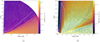 |
Fig. 2 Both panels are based on the simulation X-bn-h, time averaged from 555 to 714 yr. The white line represents the sonic surface in the wind flow, and the blue field lines correspond to the velocity stream lines. Panel b: mass flux ρv2. Within ≈3 au, a significantly lower mass flux is visible. The photoevaporation simulations are only carried out for one hemisphere. |
4 Results
Before employing the whole model including MHD terms, the photoevaporation approach was tested and compared to previous work. For this purpose, hydrodynamic simulations were carried out to study the wind topology and mass-loss rates.
The hydrodynamic stability of the disk setup was tested up to 104 Ω−1 with EUV and X-ray heating switched off and no magnetic fields. No wind or outflow forms in these conditions.
4.1 Photoevaporation
An approximately stationary flow configuration is reached within the simulation time frame (in addition to fluctuations in the upper disk atmospheresbeyond ≈60 au). Time-averaged results from 555 to 714 yr of run X-bn-h are shown in Fig. 2. When we consider the topology of the poloidal velocity streamlines, the velocity field resembles a radial field and exhibits no turbulent features toward the outer radial simulation boundary. Based on examining the sonic surface, visualized as a white line in the two plots, we state that the flow becomes supersonic, close to the wind-launching front.
Similar properties have been observed by Owen et al. (2010). Slightly different wind-loss rates can be caused by a difference in the underlying disk model and the chosen resolution. Additionally, no exponential cutoff was applied in the simulations here. Because the runs, including two hemispheres, were restricted to an outer radius of 60 au, the wind-loss rates are expected to be lower but the difference should be small because most of the wind mass-flux occurs at smaller radii. When the results of simulation X-bn-h are averaged, the total mass-loss rate produced by the wind flow is (1.38 ± 0.06) × 10−8M⊙ yr−1, which agrees well with the rates of Owen et al. (2010) (1.4 × 10⁻⁸M⊙ yr−1).
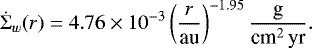
Figure 3 shows the cumulative mass-loss rate versus the cylindrical radius r. The methodhere is to trace down the stream lines of the time-averaged flow to the wind-launching front and evaluate theradius at that point. The result indicates a very smooth profile, and it is clearly visible that within 15 au, half of the mass loss occurs.
In Fig. 4 we plot the vertically integrated column density loss. Small errors in the estimation of the wind-launching front are possible because the gas trajectories do not necessarily stop at the ionization front, and it is challenging to exactly trace the origin computationally. For radii smaller than 5 au, the losses diverge from the approximate power law. In the outer part, deviations could originate from fluctuations near the boundary because the disk is observed to fail to reach static equilibrium there. For most of the simulated region, a power law of the following form can be fit:
 (30)
(30)
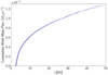 |
Fig. 3 Cumulative wind mass-loss rate in dependence of the radius in the mid-plane, resulting from time-averaged flows from 3.5 × 10⁴ Ω−1 to 4.5 × 10⁴ Ω−1. It shows that approximately half of the mass loss occurs within 15 au. |
 |
Fig. 4 Column density loss in g cm−2 and years with a fitted power law. Within 5 au, the wind rate clearly diverges from the power law, which is also true in the region near the outer simulation boundary. The two green lines represent the one-sigma margin of the fit result. |
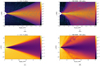 |
Fig. 5 Panels a and b: number density in cm−3 and the magnetic field lines of simulation X-b5 in the initial configuration and after an evolution of 158 inner orbits at r = r0 (≈ 1.8 orbits at 20 au), where a strong wind emerges. A slightly asymmetric flow forms in the inner region. Panels c and d: ionization fraction xe in the disk. The snapshot after 158 orbits at r = r0 visualizes the reduced ionization fraction due to the thick wind flow. |
4.2 MHD simulations
When magnetic fields are introduced into the simulations, a variety of complex phenomena are added that can drastically alter the topology of the emergent flow structure. To determine the influence of MHD effects, a study with different values of the plasma parameter ranging from 105 to 1010 was performed (see Table 1). In the following section we examine the mass flux carried by the wind sand flow structure, and we study the evolution of the magnetic field.
4.2.1 Wind flow
The magnetic field topology of run X-b5 is shown in the initial configuration and after an evolution of 158 inner orbits in Fig. 5. Clearly, the magnetic field lines are bent outward and have an inclination of more than 30° with respect to the rotation axis. In the latter snapshot, a slightly irregular outflow is visible. In the inner region of the disk an asymmetric distribution of gas develops over time due to the increasingly wound up toroidal magnetic field toward the mid-plane.
The disk remains mostly laminar in the lower atmosphere, whereas radial perturbations of the magnetic field form in the upper layers. A development of the MRI cannot be excluded, but in a 2.5D framework, the saturation of the MRI cannot be accurately followed. A more detailed discussion and the impact of the numerical resolution of the MRI modes on the wind solution is given in Sect. 4.3.
In Fig. 6 the wind structure in the upper hemisphere is displayed for simulation X-b5. Within a cylindrical radius of r ≈ 5 au, the magnetic and velocity field roughly coincide, whereas for outer radii, significant differences in the flow structure are visible, indicating that the flow is not in steady state. Figures 5c and d show the ionization fraction for the initial snapshot and after more than 150 orbits, respectively. The thick wind layer in the inner part of the disk partly blocks the radially penetrating radiation. For a wide range of the outer disk, the ionization fraction is therefore significantly lower than the optically thin region. In the two figures, thermal ionization is not taken into account (the regions with xe > 10−4 would be approximately fully ionized because of the photoevaporation temperature prescription).
In Fig. 7 we show the evolution of the wind rate over time. The mass-loss rates generally increase with lower plasma beta. For β = 105 the convergence to steady state is relatively slow because the increasing toroidal field alters the structure from the inner disk outward. At about β ≈ 107, saturation into a mostly thermally driven flow is reached. For weaker magnetic fields, fluctuations are still present because the photoevaporative flow is sensitive to changes of the vertical extent of the inner disk. Chunks of gas moving to the upper layers inhibit the irradiation of outer parts of the disk and alter the effectiveness of the heating prescription.
Figure 8 can be considered as the main result of this work. We show wind mass fluxes versus the initial plasma beta. The green region indicates the mass flux observed in the ideal photoevaporation run X-bn. The orange dashed line represents a mass-loss rate taken from the simulations of Béthune et al. (2017), which scales as 3 × 10⁻⁵β−1∕2 M⊙ yr−1. A similar relation has also been observed in the shearing box simulations of Bai & Stone (2013a). Here, the measured mass-loss rates are higher than those obtained by Béthune (see Table 2 for numerical values). On the one hand, differences in the disk model can account for the discrepancy. On the other hand, ambipolar diffusion, dominating in the upper layers of the disk, would likely lower the mass-loss rates, as observed in Gressel et al. (2015).
For β > 107 the results clearly diverge from the fitted relation and approach a saturation point that corresponds to the photoevaporation rate without magnetic fields. A magnetically driven wind cannot be launched at these initial field strengths, but the perturbations in the upper layers of the disk are still able to alter the thermal wind flow. These stochastic deviations of the mass-loss rate are visible in Fig. 7. The photoevaporation rate is about 30% lower than the result of X-bn-h because the simulation domain is smaller.
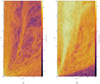 |
Fig. 6 Left panel: magnetic field structure (LIC) is visualized for simulation X-b5 after 158 yr. Only the upper hemisphere (both are simulated) is shown to highlight a larger portion of the wind structure. The color map represents the absolute poloidal magnetic flux density in Gauss. Right panel: velocity profile is depicted, including the color as the absolute velocity in cgs units. The wind is not in a steady state, as the irregular magnetic field lines and stream lines indicate. |
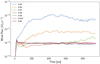 |
Fig. 7 Wind mass fluxes in solar masses per year for various simulation runs. For a plasma beta higher or lower than 107, wind rates of about one order of magnitude higher than the photoevaporation rates are observed. For a plasma beta larger than 107, lower wind rates emerge, which is an indirect result of radiation shadowing that is caused by slight magnetically induced turbulence in the inner disk region. |
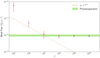 |
Fig. 8 Time-averaged wind fluxes vs. the plasma parameter β. The errorsare estimated through the standard deviation of the time -averaged sample. For stronger fields, the rates approximately follow the same power law as the dashed line, which is based on results of Béthune et al. (2017). For weaker fields, the photoevaporation begins to dominate, and the data points at β > 107 indicate the influence of radiation shielding in the inner region, which results in lower mass fluxes overall. |
Wind and accretion rates.
4.2.2 Magnetic field evolution
In the following, we pursue a more detailed study of flow properties and magnetic field evolution. All figures and studies are based on simulation run X-b5.
The two diagrams a and b in Fig. 9 show the ohmic Elsasser number ΛΩ and the local plasma beta versus the vertical height, scaled to the initial pressure scale height, for different radii. Within ≈ 3.5H, the Elsasser numbers are initially smaller than one, where MRI is expected to be suppressed by the ohmic diffusion, see Wardle (2007). The plasma beta decreases below unity in the upper layers because of the vertically exponential density and pressure distribution. For larger radii, the Elsasser numbers increase in the mid-plane because of lower densities and larger ionization fractions. In the time-averaged evolution in diagram b, ΛΩ decreases in run X-b5 at inner radii in the lower hemisphere where the asymmetric density structure builds up. The value of β increases in the inner region because the toroidal magnetic field strength becomes amplified during its evolution.
Figure 10 displays the evolution of the toroidal magnetic field. Initially zero, the field winds up as a result of Keplerianmotion and vertical shear in the layer farther away from the mid-plane. The increasing toroidal field in the mid-plane causes the asymmetric polarity distribution in vertical direction, as also observed in Béthune et al. (2017). Slightly irregular flow structures and magnetic field lines are apparent. The origin may be attributed to MRI. A saturation cannot be achieved in 2.5D dimensions, and fully developed turbulence is absent in the simulations presented here. In addition, experimenting with the boundary conditions, for instance, setting the toroidal magnetic field component to zero in the ghost cells of the inner radial boundary does not change the observed phenomena significantly.
4.2.3 Flow analysis
To examine the wind properties, we traced various variables through a poloidal (r, z) streamline in the flow. Again, run X-b5 serves as a reference model here. The actual 3D trajectory of the gas differs from the poloidal streamline because the azimuthal velocity component is zero. In this context, the streamlines are only well defined in a truly steady-state flow. Nonetheless, we used the concept of streamlines to gain insight into the flow patterns and the contributing forces.
All the following plots were computed using the same integrated streamline in their respective simulations. In Figs. 11 and 12 we show the poloidal velocities along a streamline in a time-averaged flow of X-b5, originating from (r = 6, z = 1.3) au, where v+ and v− are the fast and slow mangetosonic velocities,
![Mathematical equation: \begin{equation*} v_{\pm} = \frac{1}{2} \left[ (c_{\textrm{s}}^2 + v_A^2) \pm \sqrt{(c_{\textrm{s}}^2 + v_{\textrm{A}}^2)^2 - 4 c_{\textrm{s}}^2 v_{\textrm{Ap}}^2} \right] ,\end{equation*}](/articles/aa/full_html/2020/01/aa34945-18/aa34945-18-eq37.png) (31)
(31)
with the poloidal Alfvén velocity vAp. The Alfvén point is reached close to the wind-launching front, as well as the sonic point. At z ≈ 28 au, the poloidal flow velocity passes through the fast magnetosonic point. The definition of the wind-launching front for arbitrary radii is difficult in this case because the surface structure of the disk is rather chaotic. The streamline studied here merely acts as an example of the flow and indicates a rough position of relevant characteristic points along the wind flow.
We focus on acceleration along the streamline. Figures 13 and 14 provide further insight. In the context of the total acceleration ap, the contributing terms are (motivated by Bai et al. 2016)
![Mathematical equation: \begin{equation*} a_{\textrm{p}} = - a_{\textrm{lor}} - \frac{1}{\rho} \frac{\textrm{d}P}{\textrm{d}s} + \left[ \frac{v_{\phi}^2}{r} \frac{\textrm{d}r}{\textrm{d}s} - \frac{\textrm{d} \Phi}{\textrm{d} s} \right] ,\end{equation*}](/articles/aa/full_html/2020/01/aa34945-18/aa34945-18-eq38.png) (32)
(32)
where ds is an infinitesimally small line segment, tangential to the local streamline. The first term represents the acceleration by the Lorentz force alor in the diagrams, whereas the acceleration by the pressure force corresponds to aprs. The third term can be considered as the excess of the centrifugal over the gravitational acceleration and is labeled acen in the plots.
The magnetic term alor can be expressed in the following way:
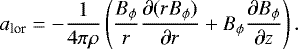 (33)
(33)
The simplification made here is to neglect the possible magnetic tension forces contributed by the poloidal field. This approach is valid, as can be examined in Fig. 15. Interestingly, the toroidal field is significantly stronger than the poloidal component for the whole streamline. Because a plasma beta of 105 still corresponds to a relatively weak field, the shearing rotation strongly winds up the poloidal field. The approximation of only considering the magnetic pressure gradient originating from the azimuthal field is therefore reasonable. Additionally, no forces due to the poloidal pressure gradient are considered here. For simulation X-b5, the magnetic acceleration effects are clearly visible along the specific streamline.Additionally, acen is negative throughout the whole flow along the streamline as a result of the sub-Keplerian motion of the gas in the upper layers of the disk atmosphere where the wind-launching front is located. This leads to the conclusion that magnetocentrifugal acceleration is not present and that the magnetic and thermal pressure gradients are the driving factors for wind acceleration. The same conclusion was drawn in Bai (2017). A reason for this phenomenon is the relatively weak poloidal field, which cannot sustain corotation to enforce magnetocentrifugal acceleration. Moreover, the Alfvén point, located closely to the wind-launching front, is consistent with this view.
The picture changes when the magnetic pressure is weaker than thermal pressure. As an example, accelerations along a streamline of the flow in run X-b10 with an initial β = 1010 are shown in Fig. 14. The dominant acceleration mechanism is the thermal pressure gradient, and magnetic contribution is negligible throughout the whole streamline. The result is consistent with the previous discussion and wind rates because simulation X-b10 is essentially equivalent to a photoevaporation run without magnetic fields.
 |
Fig. 9 Panels a and b: vertical distribution of the Elsasser number ΛΩ and the plasma beta for different radii at an initial β = 105 in the mid-plane. Second panel: time- averaged evolved state. |
4.3 Analysis of the transition region
A further analysis of the transition between the magnetically and thermally dominated wind regime is given in this section. Figure 16 shows radial column density contours as well as contours of the local plasma beta. Because the density of the magnetically launched wind decreases with increasing β, the critical column density considered for the photoevaporation heating (5 × 1022 cm−2) moves closer to the wind-launching region in the upper disk layers. The launching region roughly coincides with the β = 1 surface when the wind is magnetically driven. Within a range of 107 ≤ β ≤ 108, the critical column density lies below the upper β = 1 surface. In the case of β = 108, the magnetic field is too weak to eject material to regions far from the disk surface. The two surfaces of β = 1 are therefore located close to each other for each hemisphere. In regard to this transition occurring at the same magnetic field strengths as the saturation of the wind rates toward the photoevaporation rates, we can postulate the following: when the β =1 surface is located below the critical photoevaporation column density, the wind is predominantly magnetically driven and drives higher mass-loss rates than the thermally driven wind. When the critical photoevaporation column density lies below the β =1 surface, however, the wind can be considered to be mainly thermally driven, with a wind rate equal to the photoevaporation rate, and not being dependent on the magnetic field strength in this regime.
It might be argued that the decreasing wind rate in the magnetic regime could be caused by a lack of sufficient numerical resolution with respect to the most unstable MRI mode. However, the wind launching should not rely on MRI because it is launched by the thermal and magnetic pressure gradient (see Sect. 4.2.3).
In the following we justify this argument. The wavelength of the fastest growing MRI mode λmax is given by 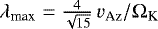 (Balbus & Hawley 1991) with the vertical Alfvén velocity vAz. We define the quality factor qMRI = λmax∕Δz. For values of β of (105;107;1010), this ratio becomes (4.95, 0.495, 0.0156). The corresponding local values of the primitive variables are taken at a height of 3H, which is located approximately at the wind-launching front. The numerical resolution is therefore clearly not sufficient to resolve effects of the MRI throughout the whole parameter range.
In order to justify the independence of the wind-launching mechanism of these numerical caveats, we performed a simulation with the same initial parameters as run X-b6, but with a lower resolution of 200 × 200 in radius and polar angle (X-b6-mri). The radial grid was again logarithmically scaled, but we chose a uniformly spaced grid in polar direction. With this setup, the quality factor becomes qMRI ≈ 0.3.
Applying the same averaging and wind rate calculation as for the previous runs, we obtained a mass-loss rate of (6.24 ± 2.56) × 10−8 M⊙ yr−1. Given the low resolution, the result agrees well with the mass-loss rate of X-b6. We can thus conclude that the numerical resolution ofMRI modes cannot account for the transition between magnetically driven disk winds and photoevaporation in our simulations.
 |
Fig. 10 Development of the toroidal magnetic field in the inner disk region in cgs units of simulation X-b5. The lines refer to the poloidal magnetic field lines. |
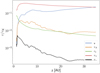 |
Fig. 11 Relevant poloidal velocities developing along a streamline in the time-averaged flow of X-b5. All velocities are normalized with the Keplerian velocity at the corresponding foot-point radius. Both the Alfvén point and the fast magnetosonic point are contained within the simulation domain. The blue line indicates the actual poloidal velocity, vA the local Alfvén speed, cs the sound speed, and v± the fast and slow magnetosonic speed. |
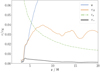 |
Fig. 12 Zoomed-in perspective of the same streamline as in Fig. 11. This resolves the location of the Alfvén point, which lies relatively close to the wind-launching front. |
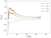 |
Fig. 13 Decomposition of the contributing accelerations along a poloidal streamline for run Xb-5. Here, acen denotes the inertial acceleration, aprs the acceleration due to the thermal pressure gradient, and alor the acceleration by the magnetic pressure gradient. |
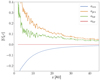 |
Fig. 14 Decomposition of the contributing accelerations along a poloidal streamline for run Xb-10. Here, acen denotes the inertial acceleration, aprs the acceleration due to the thermal pressure gradient, and alor the acceleration by the magnetic pressure gradient. |
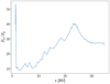 |
Fig. 15 Ratio of the toroidal and the poloidal magnetic field along a streamline in the time-averaged flow of X-b5. The toroidal field is clearly stronger by about one order of magnitude throughout the whole flow in the domain. |
4.4 Accretion rate and lever arm
In Table 2 we list the accretion rates measured for all simulation runs, including magnetic fields. The rates computed from time-averaged flows with a radial mean range from 5 to 10 au. Clearly, the accretion rates are significantly lower than the corresponding wind rates. Especially for β ≥ 107 the ratio increases to more than one order of magnitude. In contrast to β = 105 and β = 106, the streamlines in Fig. 16 show no coherent accretion flow at values of β beyond the transition toward a thermally driven wind. For stronger fields the accretion flow dissolves in the region within ≈ 3−4 au, where a more complex and stronger toroidal magnetic field is present (see Fig. 10).
Accretion rates lower than the wind rates were also observed by Gressel et al. (2015). Overall, the authors measured higher wind rates than accretion rates. A similar picture emerged in Bai (2017). In his model the accretion rate was about 2 × 10⁻⁸ M⊙ yr−1. The difference between the results of these two works and ours could be attributed to the alternative approach in the chemical model and the elevated ionization rate, as well as to the restriction to ohmic diffusion.
We verified that both radial and vertical Maxwell stresses were present in the simulations. As an example, the radial Maxwell stresses are plotted in Fig. 17 for different positions along the radial direction. The stresses are most prominent in the upper surface layers beyond one scale height. Closer to the mid-plane, ohmic diffusion inhibits these stresses. In Fig. 18 the vertical Maxwell stresses at three scale heights are displayed for the upper and lower surface. Because the magnetic field structure is rather complex, a calculation of the accretion rate by both radial and vertical stresses, taken at the positions here, would be unreliable. However, the stresses indicate that the magnetic field indeed transports momentum in the strong-field simulations. For simulation X-b5, we measured the magnetic lever arm. Streamlines were traced starting from three scale heights until the poloidal gas velocity became super-Alfvénic. The procedure was carried out over a region of 5.5 au to 12 au, resulting in a lever arm of λ = 1.06 ± 0.03. Bai (2017) reported a value of 1.15for the same β = 105. Figures 11 and 12 confirm that the wind basically starts super-Alfvénic, leading to the small lever arm.
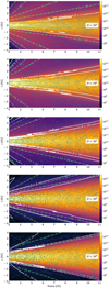 |
Fig. 16 Time-averaged flows with varying initial values of β in the mid-plane. The green dash-dotted line represents the radial column density in cm−2. The white lines mark contours of the local plasma beta. In all plots the blue arrowed lines trace velocity stream lines of the flow. The color map indicates the number density of the gas. |
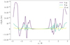 |
Fig. 17 Tree lines represent the radial Maxwell stresses in cgs units. The stresses are mostly positive and stronger toward inner radii and in the upper layers of the disk. In the mid-plane stresses are suppressed by ohmic diffusion. |
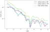 |
Fig. 18 Magnetic surface stresses (cgs units) are evaluated at three pressure scale heights for a range of 5–11 au. The lower and upper surface and their sum are represented by the three lines. |
5 Discussion
The imposed parameter space of β is sufficient to display the two regimes of photoevaporation and magnetically driven disk winds, indicated by the mass that is carried away through the wind and by the accelerations in Figs. 13 and 14. For a lower plasma beta, no completely stationary flow configuration is reached, which is represented by the evolution of the mass-loss rates in Fig. 7.
The irregular surface structure prevents a clear definition of a wind-launching front. As a proxy, the β =1 surface and the region at 3H were used. Ambipolar diffusion was observed to lower the wind mass-loss rates and to dampen the upper layers of the atmosphere (Gressel et al. 2015). The transition region between magnetically driven winds and photoevaporation would then shift toward stronger magnetic field strengths. In our simulations we did not include this effect because we aimed to extend the current photoevaporation model by Picogna et al. (2019) step by step. We reserve the inclusion of ambipolar diffusion and the Hall effect to future studies.
To compare the results with previous works, our mass-loss rates are on the same order of magnitude as those described by Béthune et al. (2017). However, the rates measured in our work are higher by a factor 3–5. This difference most likely originates from the exclusion of ambipolar diffusion here. Because Béthéthune and collaborators did not include grains in their chemical model, the ionization fraction within the disk is significantly lower in our case. A similar complex field structure emerged in the simulation of Gressel et al. (2015) without ambipolar diffusion. Their initial ohmic Elsasser number profile is comparable to that in our work.
The flow also resembles the results of simulations with β = 5000 in Sheikhnezami et al. (2012), where for this value of the plasma parameter, magnetocentrifugal effects play a minor role. The authors approached the Blandford-Payne regime for smaller β down to 10. Thus, the minimum plasma parameter of 105 applied in our simulations lies far from the transition to magnetocentrifugal winds. The observed outflows in our work do not provide a significantly large lever arm (λ ≈ 1.06).
Radial and vertical stresses are present in our models, however, and drive relatively weak accretion flows compared to the wind rates in the strong-field limit. The accretion rates for β ≥ 108 saturate to a low level of ≈2 × 10⁻¹⁰ M⊙ yr−1. These rates are most likely of numerical origin because no explicit viscosity is applied in the simulations. Numeric diffusion might lead to these nonzero net fluxes.
Bai (2017) used a similar plasma beta range and identified the magnetic pressure gradient as the main wind-launching mechanism. They reported that by applying an increasingly strong magnetic field on a purely thermal disk wind, a transition from magnetic pressure driven to magneto-centrifugally driven winds is to be expected. Very recently, Wang et al. (2019) introduced a consistent thermochemical model to the framework of Bai (2017). In contrast to the simulations performed here, no wide plasma parameter sweep was conducted. The measured wind rates are about one order of magnitude lower than in model X-b5.
In the 2D framework, MRI activity is not realistically represented, especially the development of the toroidal magnetic field. A proper study in three dimensions is required to follow the evolution more accurately. However, the inclusion of ambipolar diffusion might suppress MRI in the upper layers (or at least provide a more steady wind), as also observed by the previously mentioned authors.
We based our focus on EUV and X-ray radiation as the driving component for photoevaporation on the findings of Ercolano et al. (2009). They argued that heating by X-ray photons is dominant and leads to higher mass-loss rates than EUV heating.
6 Conclusion
We presented simulations that systematically studied the transition region between photoevaporation and magnetically driven disk winds involving a fully global 2.5D axisymmetric and nonideal magnetohydrodynamic framework. Our model includes heating by EUV and X-ray radiation and ionization by direct and scattered X-rays as well as cosmic rays. The main results can be summarized as follows:
- 1.
A magnetothermal wind without magnetocentrifugal acceleration emerges for a plasma beta of β = 105–107, leading to wind rates of about 10−8−10−7 M⊙ yr−1.
- 2.
The transition region is identified to be in the range of β ≥ 107, where the wind rates deviate from a power-law dependence on the initial plasma beta and saturate toward the pure photoevaporation rate. The transition occurs when the critical photoevaporation column density approaches the β = 1 surface. This surface roughly corresponds to the wind-launching surface in the magnetically driven wind scenario. For β = 105−106 the wind is optically thick with respect to the ionization heating. When β > 107, the critical photoevaporation column density surface lies below the region of β = 1 and the wind becomes dominantly thermally driven.
- 3.
The photoevaporation flow is sensitive to small perturbations caused by the magnetic field in the upper disk layers. Fluctuations in these regions temporarily alter the radial column densities and prevent the surface layers in the outer region from being heated by the EUV and X-ray radiation. The photoevaporation rate without magnetic fields is (9.66 ± 0.44) × 10−8 M⊙ yr−1.
Because magnetic field strengths for observed stellar systems are still uncertain (Fang et al. 2018; Vlemmings et al. 2019), it is still difficult to evaluate the importance of magnetic versus photoevaporative winds. Our results show that the transition between these two wind-launching mechanisms strongly depends on the magnetization of the disk. Our work serves as motivation for better measurements of B fields, however. Alternatively, when more wind fluxes will have been measured, the underlying values of β may be reverse-engineered based on our simulations.
Acknowledgements
P.R. wants to thank Giovanni Picogna and Barbara Ercolano for helpful discussions regarding the ionization and heating model. Additionally, P.R. thanks Giovanni Picogna for providing the X-ray photoionization temperatures. P.R. acknowledges the support of the DFG Research Unit “Transition Disks” (FOR 2634/1, DU 414/23-1). The simulations for the project were performed on the ISAAC cluster owned by the MPIA and the HYDRA and DRACO clusters of the Max-Planck-Society, both hosted at the Max-Planck Computing and Data Facility in Garching (Germany).
References
- Adams, F. C., Hollenbach, D., Laughlin, G., & Gorti, U. 2004, ApJ, 611, 360 [NASA ADS] [CrossRef] [Google Scholar]
- Bai, X.-N. 2011, ApJ, 739, 50 [NASA ADS] [CrossRef] [Google Scholar]
- Bai, X.-N. 2016, ApJ, 821, 80 [Google Scholar]
- Bai, X.-N. 2017, ApJ, 845, 75 [NASA ADS] [CrossRef] [Google Scholar]
- Bai, X.-N., & Stone, J. M. 2013a, ApJ, 767, 30 [NASA ADS] [CrossRef] [Google Scholar]
- Bai, X.-N., & Stone, J. M. 2013b, ApJ, 769, 76 [NASA ADS] [CrossRef] [Google Scholar]
- Bai, X.-N., Ye, J., Goodman, J., & Yuan, F. 2016, ApJ, 818, 152 [Google Scholar]
- Balbus, S. A., & Hawley, J. F. 1991, ApJ, 376, 214 [NASA ADS] [CrossRef] [Google Scholar]
- Béthune, W., Lesur, G., & Ferreira, J. 2017, A&A, 600, A75 [NASA ADS] [CrossRef] [EDP Sciences] [Google Scholar]
- Blaes, O. M., & Balbus, S. A. 1994, ApJ, 421, 163 [NASA ADS] [CrossRef] [Google Scholar]
- Blandford, R. D., & Payne, D. G. 1982, MNRAS, 199, 883 [NASA ADS] [CrossRef] [Google Scholar]
- Casse, F., & Keppens, R. 2002, ApJ, 581, 988 [NASA ADS] [CrossRef] [Google Scholar]
- Clarke, C. J., Gendrin, A., & Sotomayor, M. 2001, MNRAS, 328, 485 [NASA ADS] [CrossRef] [Google Scholar]
- Dedner, A., Kemm, F., Kröner, D., et al. 2002, J. Comput. Phys., 175, 645 [Google Scholar]
- Dullemond, C. P., Hollenbach, D., Kamp, I., & D’Alessio, P. 2007, in Protostars and Planets V, eds. B. Reipurth, D. Jewitt, & K. Keil (Tucson: University of Arizona Press), 555 [Google Scholar]
- Durisen, R. H., Boss, A. P., Mayer, L., et al. 2007, in Protostars and Planets V, eds. B. Reipurth, D. Jewitt, & K. Keil (Tucson: University of Arizona Press), 607 [Google Scholar]
- Dzyurkevich, N., Flock, M., Turner, N. J., Klahr, H., & Henning, T. 2010, A&A, 515, A70 [NASA ADS] [CrossRef] [EDP Sciences] [Google Scholar]
- Dzyurkevich, N., Turner, N. J., Henning, T., & Kley, W. 2013, ApJ, 765, 114 [NASA ADS] [CrossRef] [Google Scholar]
- Ercolano, B., Clarke, C. J., & Drake, J. J. 2009, ApJ, 699, 1639 [NASA ADS] [CrossRef] [Google Scholar]
- Fang, M., Pascucci, I., Edwards, S., et al. 2018, ApJ, 868, 28 [NASA ADS] [CrossRef] [Google Scholar]
- Fendt, C., & Sheikhnezami, S. 2013, ApJ, 774, 12 [NASA ADS] [CrossRef] [Google Scholar]
- Ferreira, J., & Pelletier, G. 1993, A&A, 276, 625 [NASA ADS] [Google Scholar]
- Ferreira, J., & Pelletier, G. 1995, A&A, 295, 807 [NASA ADS] [Google Scholar]
- Flock, M., Dzyurkevich, N., Klahr, H., Turner, N. J., & Henning, T. 2011, ApJ, 735, 122 [NASA ADS] [CrossRef] [Google Scholar]
- Font, A. S., McCarthy, I. G., Johnstone, D., & Ballantyne, D. R. 2004, ApJ, 607, 890 [NASA ADS] [CrossRef] [Google Scholar]
- Fromang, S., & Papaloizou, J. 2007, A&A, 476, 1113 [NASA ADS] [CrossRef] [EDP Sciences] [Google Scholar]
- Fromang, S., Latter, H., Lesur, G., & Ogilvie, G. I. 2013, A&A, 552, A71 [NASA ADS] [CrossRef] [EDP Sciences] [Google Scholar]
- Gammie, C. F. 1996, ApJ, 457, 355 [NASA ADS] [CrossRef] [Google Scholar]
- Geers, V. C., van Dishoeck, E. F., Pontoppidan, K. M., et al. 2009, A&A, 495, 837 [NASA ADS] [CrossRef] [EDP Sciences] [Google Scholar]
- Gorti, U., & Hollenbach, D. 2004, ApJ, 613, 424 [NASA ADS] [CrossRef] [Google Scholar]
- Gorti, U., & Hollenbach, D. 2009, ApJ, 690, 1539 [Google Scholar]
- Gressel, O., Turner, N. J., Nelson, R. P., & McNally, C. P. 2015, ApJ, 801, 84 [NASA ADS] [CrossRef] [Google Scholar]
- Haisch, K. E. J., Lada, E. A., & Lada, C. J. 2001, ApJ, 553, L153 [NASA ADS] [CrossRef] [Google Scholar]
- Haworth, T. J., Clarke, C. J., & Owen, J. E. 2016, MNRAS, 457, 1905 [NASA ADS] [CrossRef] [Google Scholar]
- Hayashi, C. 1981, Prog. Theor. Phys., 70, 35 [CrossRef] [Google Scholar]
- Hirose, S., & Turner, N. J. 2011, ApJ, 732, L30 [NASA ADS] [CrossRef] [Google Scholar]
- Hollenbach, D. J., & Tielens, A. G. G. M. 1999, Rev. Mod. Phys., 71, 173 [Google Scholar]
- Hollenbach, D., Johnstone, D., Lizano, S., & Shu, F. 1994, ApJ, 428, 654 [NASA ADS] [CrossRef] [Google Scholar]
- Igea, J., & Glassgold, A. E. 1999, ApJ, 518, 848 [NASA ADS] [CrossRef] [Google Scholar]
- Klahr, H. H., & Bodenheimer, P. 2003, ApJ, 582, 869 [NASA ADS] [CrossRef] [Google Scholar]
- Klahr, H., & Hubbard, A. 2014, ApJ, 788, 21 [Google Scholar]
- Lin, D. N. C., & Pringle, J. E. 1987, MNRAS, 225, 607 [NASA ADS] [CrossRef] [Google Scholar]
- Lodato, G., & Rice, W. K. M. 2004, MNRAS, 351, 630 [Google Scholar]
- Lodato, G., & Rice, W. K. M. 2005, MNRAS, 358, 1489 [NASA ADS] [CrossRef] [Google Scholar]
- Lovelace, R. V. E., Li, H., Colgate, S. A., & Nelson, A. F. 1999, ApJ, 513, 805 [NASA ADS] [CrossRef] [Google Scholar]
- Lynden-Bell, D. 1996, MNRAS, 279, 389 [NASA ADS] [CrossRef] [Google Scholar]
- Lynden-Bell, D. 2003, MNRAS, 341, 1360 [NASA ADS] [CrossRef] [Google Scholar]
- Mamajek, E. E., Meyer, M. R., Hinz, P. M., et al. 2004, ApJ, 612, 496 [NASA ADS] [CrossRef] [Google Scholar]
- Mignone, A., Bodo, G., Massaglia, S., et al. 2007, ApJS, 170, 228 [Google Scholar]
- Mignone, A., Zanni, C., Tzeferacos, P., et al. 2012, ApJS, 198, 7 [Google Scholar]
- Miyoshi, T., & Kusano, K. 2005, J. Comput. Phys., 208, 315 [NASA ADS] [CrossRef] [Google Scholar]
- Nelson, R. P., Gressel, O., & Umurhan, O. M. 2013, MNRAS, 435, 2610 [NASA ADS] [CrossRef] [Google Scholar]
- Okuzumi, S. 2009, ApJ, 698, 1122 [NASA ADS] [CrossRef] [Google Scholar]
- Owen, J. E., Ercolano, B., Clarke, C. J., & Alexander, R. D. 2010, MNRAS, 401, 1415 [NASA ADS] [CrossRef] [Google Scholar]
- Owen, J. E., Clarke, C. J., & Ercolano, B. 2012, MNRAS, 422, 1880 [NASA ADS] [CrossRef] [Google Scholar]
- Owen, J. E., Hudoba de Badyn, M., Clarke, C. J., & Robins, L. 2013, MNRAS, 436, 1430 [NASA ADS] [CrossRef] [Google Scholar]
- Paardekooper,S.-J., Baruteau, C., & Meru, F. 2011, MNRAS, 416, L65 [NASA ADS] [CrossRef] [Google Scholar]
- Pelletier, G., & Pudritz, R. E. 1992, ApJ, 394, 117 [NASA ADS] [CrossRef] [Google Scholar]
- Picogna, G., Ercolano, B., Owen, J. E., & Weber, M. L. 2019, MNRAS, 487, 691 [NASA ADS] [CrossRef] [Google Scholar]
- Pudritz, R. E., & Norman, C. A. 1983, ApJ, 274, 677 [NASA ADS] [CrossRef] [Google Scholar]
- Ribas, Á., Bouy, H., & Merín, B. 2015, A&A, 576, A52 [NASA ADS] [CrossRef] [EDP Sciences] [Google Scholar]
- Shakura, N. I., & Sunyaev, R. A. 1973, A&A, 500, 33 [Google Scholar]
- Sheikhnezami,S., Fendt, C., Porth, O., Vaidya, B., & Ghanbari, J. 2012, ApJ, 757, 65 [NASA ADS] [CrossRef] [Google Scholar]
- Stepanovs, D., & Fendt, C. 2014, ApJ, 793, 31 [NASA ADS] [CrossRef] [Google Scholar]
- Stepanovs, D., & Fendt, C. 2016, ApJ, 825, 14 [NASA ADS] [CrossRef] [Google Scholar]
- Suzuki, T. K., & Inutsuka, S.-i. 2009, ApJ, 691, L49 [NASA ADS] [CrossRef] [Google Scholar]
- Suzuki, T. K., Muto, T., & Inutsuka, S.-i. 2010, ApJ, 718, 1289 [NASA ADS] [CrossRef] [Google Scholar]
- Toomre, A. 1964, ApJ, 139, 1217 [Google Scholar]
- Turner, N. J., Sano, T., & Dziourkevitch, N. 2007, ApJ, 659, 729 [NASA ADS] [CrossRef] [Google Scholar]
- Tzeferacos, P., Ferrari, A., Mignone, A., et al. 2009, MNRAS, 400, 820 [NASA ADS] [CrossRef] [Google Scholar]
- Umebayashi, T., & Nakano, T. 2009, ApJ, 690, 69 [NASA ADS] [CrossRef] [Google Scholar]
- Vlemmings, W. H. T., Lankhaar, B., Cazzoletti, P., et al. 2019, A&A, 624, L7 [NASA ADS] [CrossRef] [EDP Sciences] [Google Scholar]
- Wang, L., Bai, X.-N., & Goodman, J. 2019, ApJ, 874, 90 [NASA ADS] [CrossRef] [Google Scholar]
- Wardle, M. 2007, Ap&SS, 311, 35 [NASA ADS] [CrossRef] [Google Scholar]
- Wardle, M., & Koenigl, A. 1993, ApJ, 410, 218 [NASA ADS] [CrossRef] [Google Scholar]
- Zanni, C., Ferrari, A., Rosner, R., Bodo, G., & Massaglia, S. 2007, A&A, 469, 811 [NASA ADS] [CrossRef] [EDP Sciences] [Google Scholar]
All Tables
All Figures
|
Fig. 1 Ionization parameter–temperature relation based on the data in Picogna et al. (2019). |
| In the text | |
|
Fig. 2 Both panels are based on the simulation X-bn-h, time averaged from 555 to 714 yr. The white line represents the sonic surface in the wind flow, and the blue field lines correspond to the velocity stream lines. Panel b: mass flux ρv2. Within ≈3 au, a significantly lower mass flux is visible. The photoevaporation simulations are only carried out for one hemisphere. |
| In the text | |
|
Fig. 3 Cumulative wind mass-loss rate in dependence of the radius in the mid-plane, resulting from time-averaged flows from 3.5 × 10⁴ Ω−1 to 4.5 × 10⁴ Ω−1. It shows that approximately half of the mass loss occurs within 15 au. |
| In the text | |
|
Fig. 4 Column density loss in g cm−2 and years with a fitted power law. Within 5 au, the wind rate clearly diverges from the power law, which is also true in the region near the outer simulation boundary. The two green lines represent the one-sigma margin of the fit result. |
| In the text | |
|
Fig. 5 Panels a and b: number density in cm−3 and the magnetic field lines of simulation X-b5 in the initial configuration and after an evolution of 158 inner orbits at r = r0 (≈ 1.8 orbits at 20 au), where a strong wind emerges. A slightly asymmetric flow forms in the inner region. Panels c and d: ionization fraction xe in the disk. The snapshot after 158 orbits at r = r0 visualizes the reduced ionization fraction due to the thick wind flow. |
| In the text | |
|
Fig. 6 Left panel: magnetic field structure (LIC) is visualized for simulation X-b5 after 158 yr. Only the upper hemisphere (both are simulated) is shown to highlight a larger portion of the wind structure. The color map represents the absolute poloidal magnetic flux density in Gauss. Right panel: velocity profile is depicted, including the color as the absolute velocity in cgs units. The wind is not in a steady state, as the irregular magnetic field lines and stream lines indicate. |
| In the text | |
|
Fig. 7 Wind mass fluxes in solar masses per year for various simulation runs. For a plasma beta higher or lower than 107, wind rates of about one order of magnitude higher than the photoevaporation rates are observed. For a plasma beta larger than 107, lower wind rates emerge, which is an indirect result of radiation shadowing that is caused by slight magnetically induced turbulence in the inner disk region. |
| In the text | |
|
Fig. 8 Time-averaged wind fluxes vs. the plasma parameter β. The errorsare estimated through the standard deviation of the time -averaged sample. For stronger fields, the rates approximately follow the same power law as the dashed line, which is based on results of Béthune et al. (2017). For weaker fields, the photoevaporation begins to dominate, and the data points at β > 107 indicate the influence of radiation shielding in the inner region, which results in lower mass fluxes overall. |
| In the text | |
|
Fig. 9 Panels a and b: vertical distribution of the Elsasser number ΛΩ and the plasma beta for different radii at an initial β = 105 in the mid-plane. Second panel: time- averaged evolved state. |
| In the text | |
|
Fig. 10 Development of the toroidal magnetic field in the inner disk region in cgs units of simulation X-b5. The lines refer to the poloidal magnetic field lines. |
| In the text | |
|
Fig. 11 Relevant poloidal velocities developing along a streamline in the time-averaged flow of X-b5. All velocities are normalized with the Keplerian velocity at the corresponding foot-point radius. Both the Alfvén point and the fast magnetosonic point are contained within the simulation domain. The blue line indicates the actual poloidal velocity, vA the local Alfvén speed, cs the sound speed, and v± the fast and slow magnetosonic speed. |
| In the text | |
|
Fig. 12 Zoomed-in perspective of the same streamline as in Fig. 11. This resolves the location of the Alfvén point, which lies relatively close to the wind-launching front. |
| In the text | |
|
Fig. 13 Decomposition of the contributing accelerations along a poloidal streamline for run Xb-5. Here, acen denotes the inertial acceleration, aprs the acceleration due to the thermal pressure gradient, and alor the acceleration by the magnetic pressure gradient. |
| In the text | |
|
Fig. 14 Decomposition of the contributing accelerations along a poloidal streamline for run Xb-10. Here, acen denotes the inertial acceleration, aprs the acceleration due to the thermal pressure gradient, and alor the acceleration by the magnetic pressure gradient. |
| In the text | |
|
Fig. 15 Ratio of the toroidal and the poloidal magnetic field along a streamline in the time-averaged flow of X-b5. The toroidal field is clearly stronger by about one order of magnitude throughout the whole flow in the domain. |
| In the text | |
|
Fig. 16 Time-averaged flows with varying initial values of β in the mid-plane. The green dash-dotted line represents the radial column density in cm−2. The white lines mark contours of the local plasma beta. In all plots the blue arrowed lines trace velocity stream lines of the flow. The color map indicates the number density of the gas. |
| In the text | |
|
Fig. 17 Tree lines represent the radial Maxwell stresses in cgs units. The stresses are mostly positive and stronger toward inner radii and in the upper layers of the disk. In the mid-plane stresses are suppressed by ohmic diffusion. |
| In the text | |
|
Fig. 18 Magnetic surface stresses (cgs units) are evaluated at three pressure scale heights for a range of 5–11 au. The lower and upper surface and their sum are represented by the three lines. |
| In the text | |
Current usage metrics show cumulative count of Article Views (full-text article views including HTML views, PDF and ePub downloads, according to the available data) and Abstracts Views on Vision4Press platform.
Data correspond to usage on the plateform after 2015. The current usage metrics is available 48-96 hours after online publication and is updated daily on week days.
Initial download of the metrics may take a while.