| Issue |
A&A
Volume 632, December 2019
|
|
|---|---|---|
| Article Number | A107 | |
| Number of page(s) | 4 | |
| Section | Galactic structure, stellar clusters and populations | |
| DOI | https://doi.org/10.1051/0004-6361/201936455 | |
| Published online | 11 December 2019 | |
Tracing Hercules in Galactic azimuth with Gaia DR2
1
Leibniz Institut fuer Astrophysik Potsdam (AIP), An der Sterwarte 16, 14482 Potsdam, Germany
e-mail: gmonari@aip.de
2
Université de Strasbourg, CNRS UMR 7550, Observatoire astronomique de Strasbourg, 11 rue de l’Université, 67000 Strasbourg, France
3
Laboratoire Lagrange, Université Côte d’Azur, Observatoire de la Côte d’Azur, CNRS, Bd de l’Observatoire, 06304 Nice, France
4
Max-Planck-Institut für extraterrestrische Physik, Gießenbachstraße 1, 85748 Garching bei München, Germany
Received:
4
August
2019
Accepted:
4
October
2019
The second data release of the Gaia mission has revealed, in stellar velocity and action space, multiple ridges, the exact origin of which is still debated. Recently, we demonstrated that a large Galactic bar with pattern speed 39 km s−1 kpc−1 creates most of the observed ridges. Among these ridges, the Hercules moving group would then be associated with orbits trapped at the co-rotation resonance of the bar. Here we show that a distinctive prediction of such a model is that the angular momentum of Hercules at the Sun’s radius must significantly decrease with increasing Galactocentric azimuth (i.e. when getting closer to the major axis of the bar). We show that this dependence of the angular momentum of trapped orbits on the azimuth on the other hand does not happen close to the outer Lindblad resonance of a faster bar, unless the orbital distribution is still far from phase-mixed, namely for a bar perturbation younger than ∼2 Gyr. Using Gaia DR2 and Bayesian distances from the StarHorse code, and tracing the average Galactocentric radial velocity as a function of angular momentum and azimuth, we show that the Hercules angular momentum changes significantly with azimuth as expected for the co-rotation resonance of a dynamically old large bar.
Key words: Galaxy: kinematics and dynamics / Galaxy: disk / solar neighborhood / Galaxy: structure / Galaxy: evolution
© ESO 2019
1. Introduction
It has long been known that the distribution of stars in local velocity space in the solar vicinity is very far from a smooth velocity ellipsoid (e.g., Chereul et al. 1998; Dehnen 1998; Famaey et al. 2005). This observational fact has become more striking than ever with the data from the second data release of the Gaia mission (Gaia Collaboration 2018), revealing in impressive detail prominent ridges in local velocity and action space. One of these ridges is associated with the well-known structure dubbed the Hercules moving group, whose exact origin remains debated. For 20 years, it has been suspected that this moving group is associated with the resonant interactions of local stars with the central Galactic bar (Dehnen 1999, 2000). For instance, if the Sun is located just outside the outer Lindblad resonance (OLR) of the bar where stars make two epicyclic oscillations while making one retrograde rotation in the rotating bar frame, a Hercules-like moving group is generated by the linear deformation of the axisymmetric background phase-space distribution function (Monari et al. 2017a,b). This implies a bar pattern speed around Ωb ≃ 55 km s−1 kpc−1 (see also, e.g., Fux 2001; Chakrabarty 2007; Minchev et al. 2007, 2010; Quillen et al. 2011; Antoja et al. 2014; Fragkoudi et al. 2019). However, Pérez-Villegas et al. (2017) demonstrated that orbits trapped at the co-rotation resonance of the bar could also reproduce the Hercules moving group in local velocity space. This explanation would be more in line with the pattern speed deduced from the recent dynamical modeling of the stellar (Portail et al. 2017; Sanders et al. 2019; Clarke et al. 2019) and gas kinematics (Sormani et al. 2015; Li et al. 2016) in the bar–bulge region, yielding Ωb ∼ 37−41 km s−1 kpc−1. In particular, Monari et al. (2019; hereafter M19) have shown that the Galactic model of Portail et al. (2017) can reproduce, from the resonances with the bar alone, most of the observed features of the local velocity and action space: while Hercules is related to the co-rotation resonance, the so-called “horn” feature (Monari 2014; Monari et al. 2017a; Fragkoudi et al. 2019) is then associated with the 6:1 resonance of the m = 6 mode of the bar potential, and the high-velocity arch or “hat” (e.g., Hunt & Bovy 2018) is caused by the OLR of the m = 2 mode.
However, most of these structures in the phase-space distribution of the solar neighborhood can be explained by different combinations of non-axisymmetric perturbations, making their modeling degenerate (Hunt et al. 2019). For instance, if the Sun is located just outside of the bar’s OLR, Hercules is caused by the linear deformation of velocity space and orbits trapped at the OLR are responsible for the horn feature which delineates the boundary of the linear deformation zone (e.g., Fragkoudi et al. 2019), while if the Sun is located just outside the bar’s co-rotation radius, orbits trapped at co-rotation are responsible for Hercules and the horn corresponds to stars trapped at the 6:1 resonance (M19). This kind of degeneracy persists even if we extend our radial coverage: for instance, looking at the ridges in tangential velocity space versus Galactocentric radius (Monari et al. 2017b; Ramos et al. 2018; Laporte et al. 2019; Fragkoudi et al. 2019) or in action space (Trick et al. 2019a), it is not clear how to discriminate between different models (Trick et al. 2019b). However, following the ridges as a function of azimuth should in principle be a promising way to disentangle the effect of different resonances. Friske & Schönrich (2019) analyzed the ridges in the average Galactocentric radial velocity as a function of angular momentum and azimuth, not limiting themselves to the Sun’s Galactocentric radius. They concluded that all the ridges taken together, if they belonged to a single pattern, would correspond to an azimuthal wavenumber m = 4.
In this paper, we concentrate on stars in an annulus of 400 pc width, centered around the Sun, and we follow the non-zero radial velocity ridge corresponding to Hercules in angular momentum versus azimuth at this Galactocentric radius as a potential discriminant between different models for the origin of the Hercules moving group. In Sect. 2 we describe our modeling procedure for computing the stellar phase-space distribution function in the zones of resonant trapping, and the expectations for the slope of the ridge in angular momentum versus azimuth for the OLR and co-rotation resonances, respectively. In Sect. 3 we compare these theoretical expectations with Gaia data, and we conclude in Sect. 4.
2. Analytical modeling
2.1. Reduction to a pendulum
To describe the stellar phase-space distribution function (DF) in the zones of resonant trapping, we use the perturbation theory method presented in Monari et al. (2017c; M19). Hereafter, the potential of the Galaxy is the one described in Portail et al. (2017), used precisely as described in M19.
The natural phase-space coordinates to study stellar dynamics in the Galaxy are action-angle variables. In an axisymmetric Galaxy within a cylindrical coordinate system (R, ϕ, z), the three natural action coordinates to use are JR, Jϕ, Jz and the canonically conjugate angles evolve linearly with time as θi(t) = θi0 + ωit, where the fundamental orbital frequencies ωi are functions of the actions. In an equilibrium configuration, the angle coordinates of stars are phase-mixed on orbital tori that are defined by the actions alone, and the unperturbed distribution function f0 is a function of actions alone (Jeans theorem). The angles, on the other hand, indicate where each star is along its orbit, and in particular the angle θϕ is closely related to the azimuth ϕ of the star. Hereafter, we work with the epicyclic approximation to estimate actions and angles (e.g., Monari et al. 2016).
We then consider a perturbation by a Galactic bar rotating at pattern speed Ωb. At a resonance with the bar, the fundamental orbital frequencies ωR and ωϕ are such that
The co-rotation resonance corresponds to l = 0. For the m = 2 mode of the bar, the OLR corresponds to l = 1.
The key canonical transformation in our procedure is the one going from the axisymmetric angle and action variables to the “slow” and “fast” variables:
As is evident from the definition of the frequencies and that of the resonance, the slow angle θs is said to be slow because it evolves very slowly close to the resonance. For the co-rotation resonance, θs is very nearly the azimuthal angle in the bar frame. Near the resonance the slow action (namely a fraction of the specific angular momentum Jϕ) also evolves slowly, and we can average the Hamiltonian over the fast angles. Formally, such an averaging produces an exactly constant fast action. For each such fast action, the Hamiltonian for the motion of the slow angle then becomes that of a pendulum, with the slow action as canonically conjugated momentum. We can define the energy of that pendulum and thus determine whether it is librating or circulating. When the pendulum is librating, the associated orbit is said to be “trapped at the resonance”. For such a librating pendulum, we then make a new canonical transformation defining the actual action-angle variables of the pendulum itself. The trapped DF close to the resonance can then be defined as the original DF phase-mixed over those pendulum angles.
2.2. Azimuthal variations of different resonant zones
Let us now heuristically determine, for different resonances with the bar’s m = 2 mode, how the location of the trapping zone moves in local velocity space when changing the azimuthal angle to the bar in configuration space. For this, let us consider a set of trapped orbits at the azimuth of the Sun within a small annulus of Galactocentric radii around the Sun, and hence with different radial angles θR, but with similar angular momentum Jϕ. Let us now evolve these orbits in time. The radial angle is a fast-varying variable (θR = θf), hence once the radial angles have varied by a small amount (e.g., ∼π/4) along any of these orbits, their slow angle θs and action Js will have varied very little.
If we consider the (l, m) = (1, 2) OLR, Eq. (2) then implies that the azimuthal angle in the bar frame will have evolved in magnitude by ∼π/8 = 22.5°, with almost constant θs and Js. Hence we expect that orbits trapped at the OLR will remain at almost constant Jϕ = 2Js over that range of azimuthal angles to the bar in the observed data. We note that this heuristic argument becomes less and less valid for resonances with much larger values of m.
On the other hand, if we consider the (l, m) = (0, 2) co-rotation resonance, the angle to the bar becomes half the slow angle because l = 0, and this means that any significant variation of this angle to the bar will be accompanied by a similar variation (and even larger by a factor of 4) in the angular momentum Jϕ. Hence we expect the angular momentum of orbits trapped at co-rotation to significantly vary with azimuth, while this is not the case for stars trapped at the OLR.
In summary, at the OLR, the azimuthal angle of stars in the bar frame varies more quickly than their angular momentum, while qqq at co-rotation the azimuth of trapped orbits in the bar frame varies very slowly, and such variations have to be accompanied by a significant change of angular momentum.
2.3. Computing the trapped distribution function
Let us now verify the above heuristic argument of Sect. 2.2 by making a quantitative evaluation of the trapped DF using the same method as in M19. First, we define an unperturbed DF f0 that is a reasonable representation of the background distribution of disk stars in phase-space (i.e. neglecting deviations from axisymmetry, moving groups, etc.). We take it to be the quasi-isothermal DF f0(JR, Jϕ) (Binney 2010) used in M19 (see M19 for details). Then we use the action-angle variables (Js, Jf, θs, θf), defined in Eq. (2), to determine the regions of phase-space where orbits are trapped to resonances (librating pendula) and where they are not (circulating pendula). As stated before, in the vicinity of the resonant regions, the dynamics of the (θs, Js) variables is that of a pendulum, for which we can also define action-angle variables (θp, Jp). We derive the DF for the trapped/librating and circulating stars in the same way as explained in Monari et al. (2017c) and M19: (1) for the librating stars we take f = ⟨f0(Jf, Js(θp, Jp))⟩, (2) for the circulating stars f = f0(Jf, ⟨Js(θp, Jp)⟩), where ⟨ ⋅ ⟩ represents the average along θp from 0 to 2π. This allows us to compute f at different positions and velocities, directly related to actions and angles using the epicyclic approximation (see, e.g., Monari et al. 2016). We select points in configuration space at R = R0 (R0 = 8.2 kpc in the Portail et al. 2017, model), with different azimuths ϕ. The azimuth is ϕ = 0 at the Sun’s position and positive in the direction of Galactic rotation, such that a point at ϕ = 28° is aligned with the long axis of the bar in the model. In particular, we consider points equispaced in ϕ and at a distance Δϕ = 4°. For each of these points we compute f on a grid in velocity space of bin-size Δv = 5 km s−1, for −150 km s−1 < vR < 150 km s−1, and 80 km s−1 < vϕ < 320 km s−1. We then use these grids to obtain the mean vR in the (ϕ, Jϕ) space: at each of the ϕ points considered, Jϕ is given by Jϕ = R0vϕ, while the mean vR is obtained summing all the values of vR on the velocity grid corresponding to a particular vϕ (or Jϕ), weighted by f/f0. In this way, and interpolating on the grid in (ϕ, Jϕ), we obtain Fig. 1.
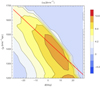 |
Fig. 1. Mean vR in the (ϕ, Jϕ) space obtained from DFs computed on velocity grids (Δv = 10 km s−1) at R = R0 and different ϕ at a distance Δϕ = 4°, using the Portail et al. (2017) model and the method described in Monari et al. (2017c) and M19 (see Sect. 2 for details). The red line corresponds to a slope of −8 km s−1 deg−1. |
Figure 1 confirms in a rigorous way what we explained hereabove with the heuristic argument. In this space, a clear ridge of positive vR appears, associated with the Hercules moving group in the model (see M19). In this model, Hercules is formed by stars trapped to the co-rotation, which, according to our heuristic argument, vary significantly in Jϕ as one varies the ϕ angle. In particular, the ridge is inclined such that Hercules shifts to lower Jϕ as we move in ϕ towards alignment with the long axis of the bar. We note that it also becomes less populated, as recently shown in the N-body simulations by D’Onghia & Aguerri (2019). These self-consistent simulations actually also displayed a displacement of Hercules with azimuth at co-rotation, which our present heuristic argument and analytic model allows us to fully confirm and physically explain. To quantify the shift in Jϕ of the co-rotation angular momentum ridge with azimuth, we overplot to the ridge a line of slope −8 km s−1 kpc deg−1 to give a rough quantitative (and yet simple) description of this trend with ϕ. Note that only the slope is relevant for the comparison we intend to make with the data, as the zero-point of the relation depends on details such as the peculiar velocity of the Sun and the slope of the Galaxy rotation curve (see M19 for details), while the exact value of the average vR depends on the choice of estimate of the action-angles (we used the epicyclic approximation here) and the form of the background DF f0.
To complete the check of the heuristic argument, we also studied the behaviour of the model when increasing the pattern speed parameter to Ωb = 50 km s−1 kpc−1, so that the OLR is slightly inside the Sun’s circle1. Also in this case ridges of negative and positive mean vR are formed in the proximity of the OLR position, and correspond in this model to the Hercules moving group (formed by stars outside the trapping region and linearly deformed by the OLR) and the horn (formed by stars inside the trapping region). In both cases the variation of the position of the ridges with ϕ is so insignificant that the ridges appear as almost straight lines of constant Jϕ, with zero slope.
3. Observational data from Gaia DR2
We now consider stars from the subset of Gaia DR2 for which RVS l.o.s. velocities are available (∼7 million stars). We use the photo-astrometric distances to these stars provided by Anders et al. (2019), obtained using the code StarHorse. We consider only the subset of stars in the sample that respects the flags recommended by the authors which corresponds to the most robust distance estimates, i.e., SHGAIAFLAG=“000” and SHOUTFLAG=“00000”. After the cleaning we are left with 6 350 087 stars.
We derive for these stars Galactocentric positions and velocities in cylindrical coordinate (R, ϕ, z), and (vR, vϕ, vz), assuming the parameters for the Sun’s distance from the Galactic centre R0 = 8.2 kpc, very close to the value of GRAVITY Collaboration (2019), Sun’s peculiar velocity w.r.t. the Local Standard of Rest (U⊙, V⊙, W⊙) = (11.1, 12.24, 7.25) km s−1, and Galaxy’s circular velocity at the Sun vc = 233.1 km s−1 (Schönrich et al. 2010; McMillan 2017). We select stars in an annulus of R such that |R − R0| < 0.2 kpc, leaving us with 1 535 484 stars, and we plot the mean vR of these stars as a function of ϕ (same convention than in Sect. 2) and Jϕ, calculating mean vR in bins of size Δϕ = 0.56° and ΔJϕ = 16 km s−1 kpc. We show this in Fig. 2.
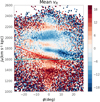 |
Fig. 2. Mean vR in the (ϕ, Jϕ) space obtained for stars from Gaia DR2, with distances estimated with StarHorse, inside an annulus of size ΔR = 0.4 kpc around R = R0. The bin sizes are Δϕ = 0.56° and ΔJϕ = 16 km s−1 kpc. The red and blue lines correspond respectively to slopes of −8 km s−1 kpc deg−1 (expected for CR) and 0 km s−1 kpc deg−1 (expected for the OLR). |
The data show prominent ridges, similar to those shown by Friske & Schönrich (2019) and Trick et al. (2019b), but this time only for stars in the small annulus. In particular the ridge corresponding to the Hercules moving group shows a displacement in Jϕ with ϕ similar to the one that we show in the model in Sect. 2. We overplot the slopes obtained from the models with trapping at CR (red line) and OLR (blue line), which show a clear agreement with the former case.
This thus demonstrates that the slope of the variation in the angular momentum of Hercules with azimuth is qualitatively in line with the signature of the co-rotation resonance of a dynamically old large bar like that of Portail et al. (2017) and Clarke et al. (2019). A key assumption of our analytical modeling is that trapped orbits are phase-mixed along the pendulum angles. In the case of an OLR origin of Hercules, the only way out would thus be to drop this assumption, hence considering that the bar is still fairly young, such that orbits are still far from phase-mixed in the bar frame. As is well known (e.g., Minchev et al. 2010), due to the initial response of the disk, a bar younger than ∼2 Gyr can cause transient features in local velocity space and displace its OLR signature with respect to the equilibrium phase-mixed case. This could indeed cause a significant variation of the angular momentum with azimuth even at the OLR, but only within the first ∼2 Gyr after bar formation (see, e.g., Fig. 7 of Trick et al. 2019b).
4. Discussion and conclusion
In this paper, we analytically demonstrated that the resonant zone associated with the co-rotation resonance of the Galactic bar should significantly vary in angular momentum as a function of azimuth at a given Galactocentric radius, while this should not happen for the OLR. Using Gaia DR2 and Bayesian distances from the StarHorse code (Anders et al. 2019), and tracing the average Galactocentric radial velocity as a function of angular momentum and azimuth, we then showed that the angular momentum of the Hercules moving group changes significantly in azimuths ranging from −20° to 20° (in an annulus of 400 pc in width around the Galactocentric radius of the Sun), as expected for orbits trapped at co-rotation in the model of M19, based on the large bar of Portail et al. (2017).
Our findings thus reinforce the case for a co-rotation origin of the Hercules moving group in the case of a dynamically old bar (> 2 Gyr). The only way for an OLR origin of the Hercules moving group to explain the observational trend reported here would be if orbits are still far from phase-mixed in the bar potential, namely for a bar perturbation younger than ∼2 Gyr. But our Fig. 2 also raises a certain number of interesting new questions that should be addressed in subsequent studies. First of all, as has been known since the publication of the Gaia DR2 catalogue (e.g., Katz et al. 2018; Trick et al. 2019a), Hercules has a secondary lower angular momentum component, whose origin is still unclear (e.g., Li & Shen 2019). This lower angular momentum ridge actually appears less inclined than the main Hercules ridge in Fig. 2, and might thus have a different origin. In addition, the horn feature, that appears as the ridge right above Hercules in Fig. 2, would correspond to the 6:1 resonance with the m = 6 mode of the bar in the model of M19. The fact that the radial velocity of the horn appears to vary very quickly with azimuth in Fig. 2, with a strongly negative radial velocity at positive azimuth and a complete disappearance of the ridge at negative azimuth, favors a resonance with such a high order mode. However, it is not clear whether the amplitude of the m = 6 mode of the bar would be sufficient to create such a prominent feature at positive azimuth. Intriguingly, the horn ridge also appears inclined: while we expect the ridges to become more inclined with higher order resonances than for the 2:1, the fact that the slope does not seem too different from the Hercules slope is intriguing. There thus remain numerous intriguing features to understand in our Fig. 2, which should be examined in future works, and it is clear that spiral arms and the recent interaction of the disk with the Sagittarius dwarf galaxy might also play a role in interpreting these kinematic features (e.g., Laporte et al. 2019). Data in a wider range of azimuths with future Gaia data releases will also allow all these potential effects to be tested further.
To be completely consistent, one should also vary the length of the bar, so that it does not extend outside the co-rotation (CR) circle. However, this is complicated to do in a model like the one of Portail et al. (2017) and the main point regarding the azimuthal behaviour of the Hercules moving group does still hold even if the model is not completely consistent.
Acknowledgments
The authors thank Elena D’Onghia and Adrian Price-Whelan for the useful discussions. BF, AS, and RI acknowledge support from the ANR project ANR-18-CE31-0006. This project has received funding from the European Research Council (ERC) under the European Union’s Horizon 2020 research and innovation programme (grant agreement No. 834148). This work has made use of data from the European Space Agency (ESA) mission Gaia (https://www.cosmos.esa.int/gaia), processed by the Gaia Data Processing and Analysis Consortium (DPAC, https://www.cosmos.esa.int/web/gaia/dpac/consortium). Funding for the DPAC has been provided by national institutions, in particular the institutions participating in the Gaia Multilateral Agreement.
References
- Anders, F., Khalatyan, A., Chiappini, C., et al. 2019, A&A, 628, A94 [NASA ADS] [CrossRef] [EDP Sciences] [Google Scholar]
- Antoja, T., Helmi, A., Dehnen, W., et al. 2014, A&A, 563, A60 [NASA ADS] [CrossRef] [EDP Sciences] [Google Scholar]
- Binney, J. 2010, MNRAS, 401, 2318 [NASA ADS] [CrossRef] [Google Scholar]
- Chakrabarty, D. 2007, A&A, 467, 145 [NASA ADS] [CrossRef] [EDP Sciences] [MathSciNet] [Google Scholar]
- Chereul, E., Creze, M., & Bienayme, O. 1998, A&A, 340, 384 [NASA ADS] [Google Scholar]
- Clarke, J. P., Wegg, C., Gerhard, O., et al. 2019, MNRAS, 489, 3519 [NASA ADS] [CrossRef] [Google Scholar]
- Dehnen, W. 1998, AJ, 115, 2384 [NASA ADS] [CrossRef] [Google Scholar]
- Dehnen, W. 1999, ApJ, 524, L35 [NASA ADS] [CrossRef] [Google Scholar]
- Dehnen, W. 2000, AJ, 119, 800 [NASA ADS] [CrossRef] [Google Scholar]
- D’Onghia, E., & Aguerri, J. A. L. 2019, ApJ, submitted [arXiv:1907.08484] [Google Scholar]
- Famaey, B., Jorissen, A., Luri, X., et al. 2005, A&A, 430, 165 [NASA ADS] [CrossRef] [EDP Sciences] [Google Scholar]
- Fragkoudi, F., Katz, D., Trick, W., et al. 2019, MNRAS, 488, 3324 [NASA ADS] [Google Scholar]
- Friske, J., & Schönrich, R. 2019, MNRAS, 490, 5414 [NASA ADS] [CrossRef] [Google Scholar]
- Fux, R. 2001, A&A, 373, 511 [NASA ADS] [CrossRef] [EDP Sciences] [Google Scholar]
- Gaia Collaboration (Brown, A. G. A., et al.) 2018, A&A, 616, A1 [NASA ADS] [CrossRef] [EDP Sciences] [Google Scholar]
- GRAVITY Collaboration 2019, A&A, 625, L10 [NASA ADS] [CrossRef] [EDP Sciences] [Google Scholar]
- Hunt, J. A. S., & Bovy, J. 2018, MNRAS, 477, 3945 [NASA ADS] [CrossRef] [Google Scholar]
- Hunt, J. A. S., Bub, M. W., Bovy, J., et al. 2019, MNRAS, 490, 1026 [NASA ADS] [CrossRef] [Google Scholar]
- Katz, D., Antoja, T., Romero-Gómez, M., et al. 2018, A&A, 616, A11 [NASA ADS] [CrossRef] [EDP Sciences] [Google Scholar]
- Laporte, C. F. P., Minchev, I., Johnston, K. V., & Gómez, F. A. 2019, MNRAS, 485, 3134 [Google Scholar]
- Li, Z., & Shen, J. 2019, arXiv e-prints [arXiv:1904.03314] [Google Scholar]
- Li, Z., Gerhard, O., Shen, J., Portail, M., & Wegg, C. 2016, ApJ, 824, 13 [NASA ADS] [CrossRef] [Google Scholar]
- McMillan, P. J. 2017, MNRAS, 465, 76 [NASA ADS] [CrossRef] [Google Scholar]
- Minchev, I., Nordhaus, J., & Quillen, A. C. 2007, ApJ, 664, L31 [NASA ADS] [CrossRef] [Google Scholar]
- Minchev, I., Boily, C., Siebert, A., & Bienayme, O. 2010, MNRAS, 407, 2122 [NASA ADS] [CrossRef] [MathSciNet] [Google Scholar]
- Monari, G. 2014, Ph.D. Thesis, Rijksuniversiteit Groningen, The Netherlands [Google Scholar]
- Monari, G., Famaey, B., & Siebert, A. 2016, MNRAS, 457, 2569 [NASA ADS] [CrossRef] [Google Scholar]
- Monari, G., Famaey, B., Siebert, A., et al. 2017a, MNRAS, 465, 1443 [NASA ADS] [CrossRef] [Google Scholar]
- Monari, G., Kawata, D., Hunt, J. A. S., & Famaey, B. 2017b, MNRAS, 466, L113 [NASA ADS] [CrossRef] [Google Scholar]
- Monari, G., Famaey, B., Fouvry, J.-B., & Binney, J. 2017c, MNRAS, 471, 4314 [NASA ADS] [CrossRef] [Google Scholar]
- Monari, G., Famaey, B., Siebert, A., Wegg, C., & Gerhard, O. 2019, A&A, 626, A41 (M19) [NASA ADS] [CrossRef] [EDP Sciences] [Google Scholar]
- Pérez-Villegas, A., Portail, M., Wegg, C., & Gerhard, O. 2017, ApJ, 840, L2 [NASA ADS] [CrossRef] [Google Scholar]
- Portail, M., Gerhard, O., Wegg, C., & Ness, M. 2017, MNRAS, 465, 1621 (P17) [NASA ADS] [CrossRef] [Google Scholar]
- Quillen, A. C., Dougherty, J., Bagley, M. B., Minchev, I., & Comparetta, J. 2011, MNRAS, 417, 762 [NASA ADS] [CrossRef] [Google Scholar]
- Ramos, P., Antoja, T., & Figueras, F. 2018, A&A, 619, A72 [NASA ADS] [CrossRef] [EDP Sciences] [Google Scholar]
- Sanders, J. L., Smith, L., & Evans, N. W. 2019, MNRAS, 488, 4552 [NASA ADS] [CrossRef] [Google Scholar]
- Schönrich, R., Binney, J., & Dehnen, W. 2010, MNRAS, 403, 1829 [NASA ADS] [CrossRef] [Google Scholar]
- Sormani, M. C., Binney, J., & Magorrian, J. 2015, MNRAS, 454, 1818 [NASA ADS] [CrossRef] [Google Scholar]
- Trick, W. H., Coronado, J., & Rix, H.-W. 2019a, MNRAS, 484, 3291 [NASA ADS] [CrossRef] [Google Scholar]
- Trick, W. H., Fragkoudi, F., Hunt, J. A. S., Mackereth, J. T., & White, S. D. M. 2019b, MNRAS, submitted [arXiv:1906.04786] [Google Scholar]
All Figures
|
Fig. 1. Mean vR in the (ϕ, Jϕ) space obtained from DFs computed on velocity grids (Δv = 10 km s−1) at R = R0 and different ϕ at a distance Δϕ = 4°, using the Portail et al. (2017) model and the method described in Monari et al. (2017c) and M19 (see Sect. 2 for details). The red line corresponds to a slope of −8 km s−1 deg−1. |
| In the text | |
|
Fig. 2. Mean vR in the (ϕ, Jϕ) space obtained for stars from Gaia DR2, with distances estimated with StarHorse, inside an annulus of size ΔR = 0.4 kpc around R = R0. The bin sizes are Δϕ = 0.56° and ΔJϕ = 16 km s−1 kpc. The red and blue lines correspond respectively to slopes of −8 km s−1 kpc deg−1 (expected for CR) and 0 km s−1 kpc deg−1 (expected for the OLR). |
| In the text | |
Current usage metrics show cumulative count of Article Views (full-text article views including HTML views, PDF and ePub downloads, according to the available data) and Abstracts Views on Vision4Press platform.
Data correspond to usage on the plateform after 2015. The current usage metrics is available 48-96 hours after online publication and is updated daily on week days.
Initial download of the metrics may take a while.