| Issue |
A&A
Volume 631, November 2019
|
|
|---|---|---|
| Article Number | A132 | |
| Number of page(s) | 9 | |
| Section | Extragalactic astronomy | |
| DOI | https://doi.org/10.1051/0004-6361/201936408 | |
| Published online | 06 November 2019 | |
Extreme ionised outflows are more common when the radio emission is compact in AGN host galaxies
1
European Southern Observatory, Karl-Schwarzschild-Str. 2, 85748 Garching, Germany
e-mail: This email address is being protected from spambots. You need JavaScript enabled to view it.
, This email address is being protected from spambots. You need JavaScript enabled to view it.
2
Max-Planck Institut für Astrophysik, Karl-Scwarzschild-Str. 1, 85748 Garching, Germany
3
Ludwig Maximilian Universität, Professor-Huber-Platz 2, 80539 Munich, Germany
Received:
30
July
2019
Accepted:
9
September
2019
Abstract
Using a sample of 2922 z < 0.2, spectroscopically identified active galactic nuclei (AGN), we explore the relationship between radio size and the prevalence of extreme ionised outflows, as traced using broad [O III] emission-line profiles in spectra obtained by the Sloan Digital Sky Survey (SDSS). To classify radio sources as compact or extended, we combined a machine-learning technique for morphological classification with size measurements from two-dimensional Gaussian models to data from all-sky radio surveys. We find that the two populations have statistically different [O III] emission-line profiles; the compact sources tend to have the most extreme gas kinematics. When the radio emission is confined within 3″ (i.e. within the spectroscopic fibre or ≲5 kpc at the median redshift), the chance of observing broad [O III] emission-line components, which are indicative of very high velocity outflows and have a full width at half-maximum > 1000 km s−1, is twice as high. This difference is greatest for the highest radio luminosity bin of log[L1.4 GHz/W Hz−1] = 23.5−24.5 where the AGN dominate the radio emission; specifically, > 1000 km s−1 components are almost four times as likely to occur when the radio emission is compact in this subsample. Our follow-up ≈0.3″–1″ resolution radio observations for a subset of targets in this luminosity range reveal that radio jets and lobes are prevalent, and suggest that compact jets might be responsible for the stronger outflows in the wider sample. Our results are limited by the available relatively shallow all-sky radio surveys, but forthcoming surveys will provide a more complete picture of the connection between radio emission and outflows. Overall, our results add to the growing body of evidence that ionised outflows and compact radio emission in highly accreting “radiative” AGN are closely connected, possibly as a result of young or weak radio jets.
Key words: galaxies: active / Galaxy: evolution / galaxies: jets / quasars: general
© ESO 2019
1. Introduction
Understanding the physical processes that connect galaxy growth and the growth of their central supermassive black holes remains one of the most important outstanding problems of galaxy evolution research (e.g. Alexander & Hickox 2012; Kormendy & Ho 2013; Heckman & Best 2014; King & Pounds 2015; Harrison 2017). The sites of growing supermassive black holes are observationally identified as active galactic nuclei because of the enormous amount of energy that they release across the electromagnetic spectrum. Cosmological models and simulations of galaxy evolution require some fraction of this released energy to couple to the surrounding interstellar medium (ISM) in order to reproduce the observed properties of massive galaxies and the surrounding intergalactic medium (IGM; e.g. Vogelsberger et al. 2014; Hirschmann et al. 2014; Crain et al. 2015; Beckmann et al. 2017; Choi et al. 2018). However, the details of how this process works in the real Universe are not well established, particularly during periods of rapid black-hole growth (e.g. Harrison 2017).
One observational strategy to establish the connection between supermassive black hole growth and galaxy evolution is to identify and characterise AGN-driven outflows in the multi-phase ISM (e.g. Veilleux et al. 2005; Morganti et al. 2005; Carniani et al. 2015; Perna et al. 2015; Brusa et al. 2015; Balmaverde et al. 2016; Rupke et al. 2017; Lansbury et al. 2018; Fluetsch et al. 2019; Ramos Almeida et al. 2019). Broad and/or asymmetrical [O III]λ5007 emission-line profiles are the most relevant to this study. They have long been used to trace outflows of warm (≈104 K) ionised gas in the narrow-line region of AGN (Heckman et al. 1984; Whittle 1985). These outflows can be located on ≈10 pc−10 kpc scales (Harrison et al. 2014; Husemann et al. 2016; Rupke et al. 2017; Villar-Martín et al. 2017; Finlez et al. 2018). This is a particularly useful outflow tracer because through large optical spectroscopic surveys such as the Sloan Digital Sky Survey (SDSS; York et al. 2000), measurements for large samples of z ≲ 0.8 AGN can be obtained (e.g. Mullaney et al. 2013; Woo et al. 2016; Zakamska & Greene 2014; Zakamska et al. 2016; Balmaverde et al. 2016). Recent and on-going near-infrared spectroscopic surveys make it possible for us to obtain similar constraints on large samples of z ≈ 1 − 3 galaxies (e.g. Harrison et al. 2016; Leung et al. 2017; Förster Schreiber et al. 2019).
Here we are particularly interested in the observations that show that the prevalence and/or velocities of [O III] outflows are related to the radio luminosity (Mullaney et al. 2013; Villar Martín et al. 2014; Zakamska & Greene 2014; Hwang et al. 2018), that is to say, that the prevalence of the most powerful outflows is higher when the radio luminosity is higher. Some authors did not find such a relationship, but their radio detection limit may have been too high. For example, Wang et al. (2018) were limited to radio luminosities of log[L1.4 GHz/W Hz−1]≳24. The relationship between outflows and radio emission may even be strongest for AGN with moderate to intermediate radio luminosities (i.e. log L1.4 GHz/W Hz−1 ≈ 23 − 25; see the discussion in e.g. Mullaney et al. 2013; Zakamska et al. 2016; Jarvis et al. 2019).
For the most radiatively luminous AGN that are sometimes called “quasars”, it is often assumed that the dominating radiative power of the central source drives the observed outflows (e.g. Faucher-Giguère & Quataert 2012; King & Pounds 2015). However, the observed relationship between outflows and radio emission opens up the possibility that the mechanical power of radio jets may be a crucial outflow-driving mechanism in these systems (e.g. Mullaney et al. 2013). From low-power AGN to the most extreme sources, radio jets are seen to interact with the ISM (e.g. Whittle et al. 1986; Ferruit et al. 1998; Tadhunter et al. 2014; Riffel et al. 2014; Kharb et al. 2017; Nesvadba et al. 2017; Finlez et al. 2018; Morganti et al. 2018; Jarvis et al. 2019). On the other hand, star formation driven outflows and quasar winds that shock the ISM provide alternative possibilities for producing the observed radio emission and correlation with outflow properties (e.g. Condon et al. 2013; Nims et al. 2015; Zakamska et al. 2016; Hwang et al. 2018; Panessa et al. 2019).
A tentative result that may shed more light on the outflow-radio connection was presented by Holt et al. (2008), who found that [O III] outflows are more extreme in compact radio galaxies (radio emission confined to within ≲10 kpc) compared to extended radio galaxies (also see Gelderman & Whittle 1994). The authors proposed that early in their evolution, radio jets strongly interact with the ISM in the nuclear regions (e.g. van Breugel et al. 1984; O’Dea et al. 1991; Bicknell et al. 2018; Mukherjee et al. 2018). However, the primary sample of Holt et al. (2008) contains only 14 sources, all of which represent the most powerful and rare radio AGN (log[L5 GHz/W Hz−1]> 26.4), and furthermore, the comparison samples are small and inhomogeneous. It is therefore not clear how applicable this result is to the bulk of the AGN population. Here we test if this result holds for more typical AGN that do not have extreme radio luminosities. We use a sample of ≈3000 targets with both [O III] emission-line profile measurements and radio size measurements.
In Sect. 2 we outline the sample selection, catalogues, and the radio data. In Sect. 3 we describe our analysis. In Sect. 4 we discuss our results, and in Sect. 5 we give our conclusions. We adopt H0 = 70 km−1 Mpc−1, ΩM = 0.3, and ΩΛ = 0.7.
2. Sample, catalogues, and radio data
We aim to explore the relationship between the extent of the radio emission and the presence of ionised outflows in AGN host galaxies. To do this, we used the value-added spectroscopic catalogue of ≈24 000 AGN that were identified in the SDSS, Data Release 7 (Abazajian et al. 2009), that was presented in Mullaney et al. (2013)1 and is consequently cross-correlated with all-sky radio surveys.
2.1. Catalogues and sample selection
The parent catalogue of Mullaney et al. (2013) contains 24 624 sources that were identified as AGN from optical spectroscopy, using a combination of emission-line flux ratios (so-called BPT diagnostics; Baldwin et al. 1981; to identify type 2 AGN) and broad Hα emission-line components (to identify type 1 AGN). For each AGN, the emission-lines, including the [O III]λ5007 line, were fit with two Gaussian components in order to search for broad emission-line components that are indicative of ionised outflows. The final sample of AGN was cross matched by Mullaney et al. (2013) with the 1.4 GHz radio surveys of Faint Images of the Radio Sky at Twenty-Centimeters (FIRST; Becker et al. 1995) and NRAO VLA Sky Survey (NVSS; Condon et al. 1998), largely following the procedure outlined in Best et al. (2005), but including sources down to a signal-to-noise ratios (S/N) > 3 in NVSS (i.e. 1.4 GHz flux densities of ≈2 mJy). Here, we used the matched catalogue as our parent sample, but we updated the FIRST radio measurements with the latest and final catalogue that is presented in Helfand et al. (2015) and contains radio sources with S/N of ≥5 (detection limit ≈1 mJy).
As in Mullaney et al. (2013), we preferred to use the NVSS flux density measurements to infer the total radio luminosity densities (L1.4 GHz) because the larger beam (full width at half-maximum, [FWHM]≈45 arcsec) compared to FIRST reduces the likelihood of resolving flux away or missing extended radio structures. However, the FIRST data with a resolution of ≈5 arcsec were used for a more accurate positional matching to the SDSS sources (Mullaney et al. 2013). Furthermore, we also used a higher spatial resolution of the FIRST data for radio size measurements and morphological classifications (see Sect. 3.2).
Starting with the parent catalogue, we created the final sample to be used in this work by applying the following criteria:
1. We only considered AGN within a redshift range of 0.02 < z < 0.2 (discussed in more detail below), leaving a sample of 16326 AGN.
2. We only considered AGN with 1.4 GHz radio detections in the FIRST or NVSS catalogues (this is required to characterise the spatial extent of the radio emission), leaving a sample of 2948 AGN.
3. We removed a small number of sources (only 0.9% of the sample) for which either (a) the two-component fits to the [O III] emission-line profiles failed to converge in the Mullaney et al. (2013) catalogue (3 targets removed), (b) the NVSS-only detections (i.e. those that are not in the FIRST catalogue) are not covered by FIRST imaging at all (which is required for our later analyses; Sect. 3.2), or that by visual inspection were associated with the wrong optical counterpart (usually mergers; 23 targets removed). This resulted in our final sample of 2922 AGN.
The upper bound of the redshift range in step (1) is a compromise between keeping a significant number of luminous AGN in the sample and having a reasonable detection limit on the radio (i.e. a limit of log[L1.4 GHz/W Hz−1]≈22.8 at the highest redshift of z = 0.2) and a reasonable physical resolution (1 arcsec corresponds to ≤3.3 kpc for z ≤ 0.2). The lower bound of z = 0.02 is such that the 3 arcsec SDSS fibre still covers a reasonable fraction of the galaxy compared to the higher redshift sources (1 arcsec corresponds to 0.4 kpc at z = 0.02). We further consider the varying physical size scales covered by the SDSS spectroscopy when we present our results in Sect. 4.2.
The final sample we used consists of 2922 AGN. The distributions of rest-frame 1.4 GHz radio luminosities and the [O III] luminosities are presented in Fig. 1. The radio and [O III] luminosities of the two samples are broadly similar. We still take these small differences into account when we compare the two populations in Sect. 4.2. We assumed a radio spectral index of α = 0.8 when we calculated the radio luminosity, where Fν ∝ ν−α, motivated by multi-frequency radio observations of a subset of this sample (Jarvis et al. 2019). We note that assuming an extreme range of spectral indices α = −0.8 to α = 1.1 (Lal & Ho 2010) has the effect of changing the radio luminosities by a median factor of −16% to +3% (maximum of −34% to +6%). However, this choice does not affect our main conclusions. Overall, the sample covers five orders of magnitude in radio luminosity, with a median of log[L1.4 GHz/W Hz−1] = 22.7, and four orders of magnitude in [O III] luminosity, with a median of log[L[O III]/erg s−1] = 41.1. Although our sample only includes sources that are radio detected and we were unable to investigate the majority of the population, which is radio undetected, our sample is dominated by AGN that are not extremely luminous in the radio (see Fig. 1). Specifically, only 4.5 % and 1.0
 % are above 1024 or 1025 W Hz−1, respectively (where the quoted range is for spectral indices varying from α = −0.8 to α = +1.1; Lal & Ho 2010).
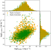 |
Fig. 1. Radio luminosity (rest-frame 1.4 GHz) vs. [O III] luminosity for our final sample of 2922 AGN. The sources we classify as having extended radio emission are shown with green empty symbols, and those we classify as radio compact sources are shown with filled orange symbols. The normalised luminosity histograms for both populations are also shown as empty and filled histograms. |
2.2. Follow-up radio observations
To aid the interpretation of our results on this large sample of 2922 AGN, we also used follow-up radio observations that we carried out with the Karl G. Jansky Very Large Array (VLA) that reach a higher spatial resolution than is achieved by the FIRST and NVSS surveys. Example data are compared to the FIRST images in Fig. 2. For our VLA observations we targeted a subset of the z < 0.2 AGN from Mullaney et al. (2013) to observe at 1.4 GHz (at ≈1 arcsec resolution) and 6 GHz (at ≈0.3 arcsec resolution). The VLA programme IDs are 13B−127, 16A−182, and 18A−300. As in this work, the targets for these programmes were selected from Mullaney et al. (2013) to be radio detected in FIRST and/or NVSS, but with an additional focus on AGN with L[O III] > 1042 erg s−1 (see discussion in Sect. 4.2). The radio images typically have root-mean-square (rms) noise values of 10−50 μJy. The first ten targets from these follow-up programmes were pre-selected to have ionised outflows and are presented in Jarvis et al. (2019). The wider sample of 42, with no pre-selection on outflows, will be presented in Jarvis et al. (in prep.). In Fig. 2 we include examples of our radio images from the full sample, with our 1.4 GHz images shown as green contours and our 6 GHz images inset with blue contours. The observing strategy and imaging techniques are described in Jarvis et al. (2019). In this work we make use of these images to qualitatively describe the radio morphologies and to also indicate which structures might be prevalent in the wider sample (e.g. radio jets; Sect. 3.2; Fig. 2).
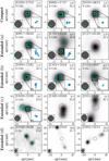 |
Fig. 2. Examples of radio images to demonstrate our classification into compact and extended radio sources (Sect. 3.2). Grey-scale images show 1.4 GHz FIRST data (≈5 arcsec resolution). Where available, green contours are from our ∼1 arcsec resolution 1.4 GHz images, and the insets are from our ∼0.3 arcsec resolution 6 GHz images (blue contours; Sect. 2.2). Synthesised beam(s) are represented by appropriately coloured ellipses. Labels provide the galaxy name (Jarvis et al. 2019; Jarvis et al., in prep.), minimum and maximum contour levels, radio sizes from FIRST (RMaj), and radio luminosities (in log[W Hz−1]). Magenta circles represent the SDSS fibre size. Compact radio sources (top row) are defined as those whose radio emission is dominated within the SDSS fibre, whilst extended sources (bottom four rows) show significant emission outside of the fibre extent. |
3. Analyses
In this work we are interested in (1) searching for high-velocity ionised gas, which is indicative of outflows, by characterising the [O III]λ5007 emission-line profiles and (2) relating the ionised gas kinematics to the spatial extent of the radio emission. In the following we describe how we characterised the [O III] emission-line profiles (Sect. 3.1) and constrained the spatial extent of the radio emission by defining each source as having either compact or extended radio emission (Sect. 3.2).
3.1. Characterising the emission-line profiles
The velocity widths of the [O III] emission-line profiles are good tracers of the ionised gas kinematics, and in particular, for identifying non-galactic motions associated with outflows (e.g. Mullaney et al. 2013; Liu et al. 2013). Here we make use of the two-component fits to the [O III] emission-line profiles provided by Mullaney et al. (2013) and characterise the velocity widths in two different ways (we show two examples in Fig. 3):
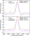 |
Fig. 3. [O III]λ5007 emission-line profiles (grey curves) and their fits (dashed curves) for an example with a single component (upper panel) and an example with two components (lower panel). The individual components A and B are shown as dot-dashed and three-dot-dashed curves, respectively, artificially offset by −0.1 in the y-axis. We considered both the velocity widths of any identified broad components (FWHMB) and the flux-weighted average line widths of all identified components (FWHMAvg) here. |
– The FWHM of the second broader component (FWHMB; see the bottom panel in Fig. 3). For 2239 of the 2922 AGN in the parent sample, that is, 77%, such a second component is required. We discuss the prevalence of high-velocity (broad) components in Sect. 4.1.
– The flux-averaged FWHM of the two Gaussian components, FWHMAvg =  , where FA and FB are the fractional fluxes contained within the two fitted components, A and B. This definition has the advantage of considering lines that are fitted either with one or two Gaussians (e.g. sources may have broad emission-line profiles but are satisfactorily fitted with only a single Gaussian; Mullaney et al. 2013, see the upper panel in Fig. 3).
We take the corresponding uncertainties on each of these velocity width values (Mullaney et al. 2013) into account when we present our results in Sect. 4.2.
3.2. Compact and extended radio emission
To separate our classifications of compact and extended radio sources, we determined for which sources the radio emission extent lies within or outside of the spatial extent of the SDSS fibre (i.e. 3 arcsec diameter). This is so that we can connect this to the observed [O III] emission-line profiles seen in the fibre spectroscopy (see above). This is required so that we can evaluate the connection of radio size and outflow in our sample of ≈3000 in the absence of spatially resolved spectroscopy (which is currently limited to considerably smaller samples; e.g. Villar-Martín et al. 2017; Jarvis et al. 2019). For the redshift range of our sample (z = 0.02−0.2), 3 arcsec corresponds to 1.2−10 kpc; but we note that our conclusions hold if we only consider sources z = 0.1−0.2, for which the physical size scale varies by less than a factor of two, and if we choose a physical size cut-off of 5 kpc (Sect. 4.2).
To characterise the extent of the radio emission, we combined two different approaches: (1) we used radio major axis sizes (Rmaj) from simple elliptical Gaussian models (Sect. 3.2.1), and (2) we used an automated morphological classification scheme (Sect. 3.2.2). It was necessary to combine these two approaches because whilst the former method has the advantage of providing a quantitative measure of the radio sizes and corresponding uncertainties, it has the disadvantage of missing structures that are not well characterised by a single elliptical Gaussian model. For example, our sample contains 89 sources that are detected by NVSS but are not in the FIRST catalogue, largely because the emission is located in large diffuse structures or off-nuclear lobes that are missed because the beam of FIRST is relatively small (e.g. see the bottom row in Fig. 2). Furthermore, in the FIRST catalogue, the fits to the images are dominated by central cores even if additional extended radio structures lie beyond the core (e.g. see rows 2 and 4 in Fig. 2).
3.2.1. Basic radio size measurements
Helfand et al. (2015) fit an elliptical Gaussian model for each source detected in their FIRST catalogue. We used these major axis sizes (RMaj), which were deconvolved for the point-spread function (or “beam”), noting that 89 sources (3% of the sample) do not have any constraints on RMaj because they only have radio detections in the NVSS catalogue (see above). Noise can cause the RMaj sizes (before deconvolution) to be smaller than the beam (see Helfand et al. 2015). For the 618 cases in our sample the corresponding deconvolved sizes are assumed to be zero (example in the second row of Fig. 2). The uncertainties in RMaj depend on the signal-to-noise ratio (S/N), following approximately σ(RMaj) = 10 × (1/(S/N) + 1/75) arcsec, where S/N = (Fpeak − 0.25)/rms, Fpeak is the peak flux density and rms is the root-mean-square noise of the image (Helfand et al. 2015). The signal-to-noise ratios are not simply Fpeak/rms because of the applied CLEAN bias correction to the peak flux density. Importantly, as demonstrated by this equation, it is possible to obtain sizes with reasonable uncertainties well below the size of the nominal point-spread-function when the sources are detected with high signal-to-noise ratios. For example, a source with an S/N = 10 has a size uncertainty of ≈1 arcsec. We take the size uncertainties into account when we present our results in Sect. 4.2. We plot the RMaj values in Fig. 4.
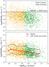 |
Fig. 4. [O III] emission-line width vs. radio size, using two definitions: (1) the velocity width of the broadest [O III] emission-line component (FWHMB; top panel) and (2) the flux-weighted average velocity width of two emission-line components (bottom panel; FWHMAvg). Symbols are colour-coded as in Fig. 1 with the addition of the curve showing the running median (in 0.1 dex bins) and the corresponding 16th and 84th percentiles in the bottom panel. The small number of radio extended sources with apparently small sizes is due to extended radio structures beyond the core (see Sect. 3.2). We see a weak trend where the largest sources with ≈8 arcsec have a 0.1−0.2 dex smaller velocity widths on average than the smaller ≈1 arcsec sources. Compact radio sources are more likely to have the broadest emission-line components (e.g. FWHMB > 1000 km s−1; above the dashed line; Sect. 4.1). |
We can also define how extended a source is in the FIRST images based on the ratio of the peak and integrated flux densities following  (Kimball & Ivezić 2008), where FInt is the integrated flux from the elliptical Gaussian models (Helfand et al. 2015). These θ values describe how resolved a source is because a higher FInt/FPeak ratio implies that the extended radio emission (e.g. radio lobes) contributes more to the total radio flux. A source in FIRST can typically be considered extended when θ ≥ 1.06 (Kimball & Ivezić 2008). We find that RMaj and θ are well correlated for our sample, with a correlation coefficient value of 0.91, and the overall conclusions presented throughout this work are insensitive to the choice of setting RMaj > 3 arcsec versus θ > 1.06 to define a source as radio extended.
3.2.2. Morphological classification
As previously described, for a complete characterisation of the sources that are compact or extended in the radio, it is important to apply a morphological classification in addition to simple sizes (e.g. to identify core-lobe structures). To do this we used the FIRST Classifier, presented in Alhassan et al. (2018), which is an automatic morphological classification tool applied to FIRST images that uses a trained, deep convolutional neural network model. The code was trained using a set of radio sources with known classifications. Sources are classified as FRI, FRII (Fanaroff and Riley class I and II; Fanaroff & Riley 1974), bent (determined to have a more complex, “bent” nature), or compact. We are not interested in the individual classifications of FRI, FRII, or bent here, and only consider whether the radio emission is extended or compact. The model achieves an overall accuracy of 97% based on control samples (Alhassan et al. 2018).
We performed our own random visual inspection to verify that the morphological classifications returned by the FIRST Classifier were reliable. Furthermore, we used the subset of our sample that was covered by our follow-up higher resolution radio observations (Sect. 2.2; Fig. 2). The FIRST Classifier was successful at identifying extended radio structures (e.g. the sources in the second and fourth row of Fig. 2). Nonetheless, sources that are smoothly extended beyond 3″ in FIRST and lack clear distinct morphological structures can be misclassified as compact by the FIRST Classifier (e.g. see the third row of Fig. 2). Therefore, we found that a combination of using RMaj and the results of the FIRST Classifier was required to reliably classify all of the sources in our sample into either radio compact or radio extended.
3.2.3. Final classification into compact and extended radio sources
As described above, we wish to define compact sources as those whose radio emission is concentrated within the SDSS fibre (i.e., ≲3 arcsec), and define sources as extended otherwise. Based on the measurements described in the previous two sub-sections, we applied the following criteria to separate the two populations:
– Compact: RMaj ≤ 3 arcsec and not identified as extended by the FIRST Classifier (1620 sources; i.e. see the first row in Fig. 2).
– Extended (a): Sources with RMaj ≤ 3 arcsec that are identified as extended by the FIRST Classifier (246 sources). Visual inspection shows that these targets typically have strong cores (which results in the small sizes from simple 2D Gaussian fits) but additional extended structures expand beyond the core. These are picked up by the FIRST Classifier (see the second row in Fig. 2).
– Extended (b): RMaj > 3 arcsec but not classified as extended by the FIRST Classifier (679 sources). Visual inspection reveals that these targets are large but do not have clear discernible features that would be picked up by the FIRST Classifier (see the third row in Fig. 2).
– Extended (c): RMaj > 3 arcsec and classified as extended by the FIRST Classifier. These sources are clearly extended with morphological structures on large scales (288 sources; see the fourth row in Fig. 2).
– Extended (d): Sources that are not detected in the FIRST catalogue but are identified in NVSS (89 sources). Visual inspection verifies that these targets are large radio sources, which are usually dominated by symmetrical lobes (see the bottom row of Fig. 2).
With these criteria, 1302 sources are classified as extended and 1620 are classified as compact in the radio. A visual inspection of the FIRST images, in combination with our follow-up radio observations (Fig. 2), provides verification that these criteria are effective at separating sources whose radio emission is dominated within 3 arcsec or extends beyond this limit. As expected, there are a few ambiguous cases within the full sample of 2922. For example, from our follow-up radio observations, J0945+1737 in the top row of Fig. 2 is known to have a weak radio structure beyond the central 3 arcsec; however, this constitutes only ≈9% of the total radio emission, and the majority of the radio emission is due to a compact ≲2 kpc central core and radio jet (Jarvis et al. 2019). Overall, we feel confident that for this statistical study our classification into compact and extended radio sources is sufficient and is likely the best that can be achieved with the current radio surveys.
The radio and [O III] luminosities for the compact and extended samples are represented as solid and empty symbols, respectively, in Fig. 1. Their median radio luminosities are log[L1.4 GHz/W Hz−1] = 22.80 and 22.67, respectively, with a standard deviation 0.7 dex in both cases. The median [O III] luminosities are log[L[O III]/erg s−1] = 41.18 and 41.03, respectively, both with a standard deviation of 0.7 dex. Although there are only small differences of ≈40% in the median radio and [O III] luminosities of the two populations, we note that we repeated all of our experiments using individual 1 dex bins of radio and [O III] luminosity to account for these differences in Sect. 4.2. With the final classifications of compact versus extended radio emission, we can now explore the relationship between radio size and ionised gas kinematics.
4. Results and discussion
To investigate the relationship between the prevalence of extreme ionised outflows and the size of the radio emission in AGN host galaxies, we constructed a sample of 2922 z = 0.02−0.2 spectroscopically identified AGN that are detected in 1.4 GHz radio images (Sect. 2.1; Fig. 1). Using a combination of direct size measurements and morphological classifications, we identified the sources that are compact and those that are extended in the radio based upon whether the radio emission is dominated within or outside of ≈3 arcsec (or ≈5 kpc at the average redshift; Sect. 3.2; Fig. 2). Two Gaussian component fits to the [O III] emission-line profiles were used to characterise the ionised gas velocities using (1) the width of any identified broad emission-line components (FWHMB), and (2) the flux-averaged width of the two components (FWHMAvg; Sect. 3.1; Fig. 3). Here we present our results on the trend between radio size and ionised gas velocities (Sect. 4.1) and with the prevalence of ionised outflows (Sect. 4.2), before we discuss the implication of our results in the context of AGN feedback and the possible physical mechanisms driving the outflows (Sect. 4.3). The quantitative results of our analyses are presented in Table 1.
Results of comparing the [O III] emission-line profiles for AGN that we classify as radio compact versus radio extended for various subsets of the sample.
4.1. Trends between ionised gas velocities and radio sizes
In Fig. 4 we plot the FWHM of the [O III] emission lines versus radio size (RMaj) for the AGN in our sample. In the bottom panel, we show the same, but using the FWHMAvg, which has the advantage of being defined for targets with one or two Gaussian component fits to the [O III] profiles (see Sect. 3.1) and gives a sense of the flux-weighted average ionised gas velocities inside the galaxy (covered by the spectroscopic fibres). A general trend that the largest radio sources typically have lower ionised gas velocities is visible: the average FWHMAvg drops by 35% from RMaj = 1 arcsec to RMaj = 8 arcsec. The top panel of Fig. 4 is easier to interpret, where the percentage of targets with a very high velocity component of FWHMB > 1000 km s−1, indicative of extreme outflows, is higher for the smaller radio sources (see the dashed line). Specifically, for targets with RMaj < 3 arcsec, 10.7% exhibit [O III] emission-line components with FWHMB > 1000 km s−1, whilst such features are half as common (5.3%) for targets with RMaj > 3 arcsec.
One important limitation of using the radio size measurements, RMaj, in Fig. 4 is that they fail to properly capture sources with large extended radio structures, which is why sources that are classified as extended (green data points) can have apparently small sizes (see Sect. 3.2). Furthermore, we have not considered the uncertainties on the size or velocity measurements so far. In the following subsection we therefore quantify the relationship between radio size and the prevalence of extreme outflows further, using our classifications of compact versus extended radio emission (Sect. 3.2) and accounting for the uncertainties.
4.2. Extreme outflows are more prevalent with compact radio emission
In the top two panels of Fig. 5 we show the cumulative distribution of FWHMAvg and FWHMB for the full AGN sample of this work. Sources that are radio compact (orange curves) typically have higher ionised gas velocities than sources that are radio extended (green curves). A two-sided Kolmogorov–Smirnov test (KS-test) comparing the radio compact sources to the radio extended sources reveals that they have FWHMAvg and FWHMB distributions that are not consistent with each other, with p-values of 3.9 × 10⁻¹⁴ and 2.7 × 10⁻¹², respectively (where a p-value < 0.05 rejects the null hypothesis that the two samples are drawn from the same distribution). Furthermore, we found that compact sources are twice as likely to have FWHMB > 1000 km s−1 emission-line components compared to extended radio sources, with 11% versus 5.7% exhibiting such components, respectively. These differences between compact and extended radio sources also remain when we focus on a narrower redshift range of z = 0.1−0.2 so that there is only a variation by a factor of 2 in the physical size scale covered by the SDSS fibre. For a full breakdown of these results, see the top two rows in Table 1. We note that if we use 5 kpc, as opposed to 3 arcsec, to define radio extended in the z = 0.1−0.2 bin we obtain extreme outflow detection fractions of 15.7% and 10.5% for compact and extended radio sources, respectively.
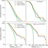 |
Fig. 5. Fraction of AGN with [O III] FWHM greater than a given value for FWHMAvg (left two panels) and FWHMB (right two panels). Top two panels: full sample of this work, and the bottom two panels show the subset with radio luminosities of log[L1.4 GHz/W Hz−1] = 23.5−24.5. The cumulative distributions are shown for all the sources in each bin (blue curves) and split by our classifications of compact and extended radio sources (orange and green curves, respectively). Extreme ionised gas velocities are more prevalent when the radio emission is compact; e.g., components with FWHMB > 1000 km s−1 are four times as likely in compact sources in the log[L1.4 GHz/W Hz−1] = 23.5−24.5 sample (bottom right panel). |
As mentioned previously, it is important for us to take the uncertainties on the radio size measurements and emission-line velocity width measurements into account. Therefore, we used a Monte Carlo approach to generate 104 sets of RMaj, FWHMB, and FWHMAvg values for the 2922 targets in our sample. To do this, we randomly perturbed the true values by their uncertainties using a normal distribution with a width equal to the measurement errors. For each of the 104 sets, we re-classified the full sample as compact or extended, following Sect. 3.2, and repeated the two-sided KS-tests on the FWHMB and FWHMAvg distributions. From this exercise we found that the 99.73 percentiles of the p-values from the 104 Monte Carlo runs are 6.6 × 10⁻⁹ and 1.7 × 10⁻⁶ for FWHMB and FWHMAvg, respectively. This shows that when the uncertainties are folded in, the ≈3σ maximum p-values still reveal that FWHMAvg and FWHMB distributions of compact and extended radio sources are not consistent with each other. Furthermore, with these same Monte Carlo runs, at most 8.5% of the compact radio sources have an FWHMB > 1000 km s−1 (again using the 99.73 percentile), which is still a smaller fraction than the 11% observed in the compact radio sources (see Table 1).
Another important consideration for interpreting our results is to confirm that the radio size or morphology drives the physical parameter on the different prevalence of extreme ionised outflows and that it is not driven by the underlying [O III] or radio luminosities (Fig. 1, Mullaney et al. 2013). To test for this, we repeated the above calculations and Monte Carlo simulations, but split the full sample into 1 dex bins of [O III] luminosity and radio luminosity. We only considered bins with > 50 sources, which meant that we were able to explore the luminosity ranges of log[L1.4 GHz/W Hz−1] = 21.5−24.5 and log[L[O III]/erg s−1] = 39.5−42.5, split into three bins in both cases. The full results of these tests can be found in Table 1. We find that for all radio luminosity bins except for the lowest bin, we can be confident that the prevalence of extreme outflows (i.e. components with FWHMB > 1000 km s−1) is higher for the compact sources (even when we account for the uncertainties; see Table 1). Furthermore, in nearly all luminosity bins the p-values consistently show that the compact and extended radio sources do not have the same FWHMAvg or FWHMB distributions, even when the uncertainties during the Monte Carlo runs are considered. The exceptions to this are the two lowest luminosity bins of log[L1.4 GHz/W Hz−1] = 21.5−22.5 and log[L[O III]/erg s−1] = 39.5−40.5, where the AGN are likely to be particularly weak and/or star-formation processes dominate the observed radio luminosities.
Exploring the effect of luminosity further, we find that the difference in ionised gas velocities between compact and extended radio sources is most significant in the largest radio luminosity range of log[L1.4 GHz/W Hz−1] = 23.5−24.5 that we considered. The FWHM cumulative distributions for this subsample are shown in the bottom two panels of Fig. 5. This result is quantified by the fact that the prevalence of FWHMB > 1000 km s−1 components is almost four times higher in the compact versus extended radio sources, compared to a factor of two for the full population. In this radio luminosity range, AGN are generally accepted to dominate the radio emission at low redshift (e.g. Kimball & Ivezić 2008; Condon et al. 2013; Mancuso et al. 2017). Following (Kennicutt & Evans 2012), when we assumed that the radio luminosities were all from star formation for the range log[L1.4 GHz/W Hz−1] = 23.5−24.5, this would correspond to star formation rates of ≈200−2000 M⊙ yr−1. At these redshifts, it would be extremely unlikely for more than one or two of the sources to have such high star-formation rates; for example, X-ray AGN have an average star-formation rate of ≈1−8 M⊙ yr−1 at z ≲ 0.5 (Stanley et al. 2015; Shimizu et al. 2017). Even more importantly, follow-up observations of subsets of the sample in this luminosity range show that star formation is very unlikely to dominate in most cases because of the observed collimated radio structures and very high radio excess (Fig. 2; Jarvis et al. 2019). However, because these high-resolution radio observations (Sect. 2.2) only represent the [O III] and radio luminosity bins where the difference between compact and extended radio sources is strongest, further high-resolution radio observations are required to establish the origin of radio emission in the overall population (also see Panessa et al. 2019).
Finally, we also considered the possibility that type 1 AGN may bias the results due to projection effects that could potentially lead to Doppler boosted radio emission, seemingly more compact radio emission, and/or higher observed outflow velocities. Therefore, we repeated our analyses only including the type 2 (type 1) AGN and found that 7.5% (27.4%) of the radio compact sources show a > 1000 km s−1 broad [O III] component and 3.6% (15.3%) of the extended sources do. The type 2 only sample has a lower detection fraction of extreme outflows, consistent with the results presented in Mullaney et al. (2013) that type 1 AGN typically have higher observed [O III] velocities, likely due to projection effects. However, this test shows that type 2 AGN alone show a consistent result with the overall sample that extreme outflows are roughly twice as common when the radio emission is compact. This is still true when we focus on the type 2 AGN in our highest radio luminosity bin, where our result is strongest (see Fig. 5). Here we find that 21.1% of the compact radio sources, compared to 8.5% for the extended radio sources, exhibit extreme [O III] components of > 1000 km s−1. It will be interesting to explore and to further understand the differences between type 1 AGN and type 2 AGN in the future using larger samples that are complete down to lower radio luminosities.
Overall, we conclude that the prevalence of extreme ionised outflows is highest when the radio emission is compact and the AGN are clearly the dominating source of radio emission (i.e. log[L1.4 GHz/W Hz−1] = 23.5−24.5). We only have small numbers of sources at higher radio luminosities; therefore, we are unable to extend our results to log[L1.4 GHz/W Hz−1]> 24.5.
4.3. Implications of our results
We find that extreme ionised outflows observed in SDSS spectroscopy for z < 0.2 AGN are more common when the radio emission is concentrated within the spatial extent of the spectroscopic fibre. This underlines the idea of a connection between radio emission and outflows in AGN (e.g. Mullaney et al. 2013; Zakamska & Greene 2014). For the sample at hand (i.e. where radio emission is detected; Sect. 2.1), we suggest that this is not driven by star formation processes because the result is strongest when AGN dominate the radio emission. Our result shows that the connection between outflows and compact radio emission for extremely radio bright AGN, found by Holt et al. (2008), is also found in AGN that are not extremely radio luminous and are therefore more representative of the overall population.
If the radio emission traces the extent of jets, our result could imply that we can see the effect of jet-ISM interactions from young radio sources or weak jets that will never escape the host galaxy (e.g. van Breugel et al. 1984; O’Dea et al. 1991; O’Dea 1998; Morganti 2017; Bicknell et al. 2018). Where larger scale jets deposit their energy outside of the region that is covered by the spectroscopic fibre, the spectroscopic measurements do not cover the physical region of jet-ISM interactions.
In favour of the jet scenario, we see collimated jet-like features (including hot spots and bent jets) in our follow-up high-resolution radio observations (Fig. 2; Jarvis et al. 2019). Furthermore, spatially resolved spectroscopic observations reveal jet-ISM interactions in sources with a range of jet powers, particularly on the scale of the galaxy bulges (i.e. a few kiloparsec; Tadhunter 2016; Villar-Martín et al. 2017; Jarvis et al. 2019; Husemann et al. 2019a,b). Spatially resolved spectroscopic observations are also crucial for decoupling less extreme ionised outflows from galactic kinematics; here we were only able to confidently identify the most extreme cases.
The most recent simulations show that compact jets that interact with a clumpy ISM may be a crucial aspect of AGN feedback and may be the most efficient mechanism for driving powerful outflows (e.g. Wagner et al. 2012; Mukherjee et al. 2016; Bicknell et al. 2018; Cielo et al. 2018). Alternatively, the increased prevalence of extreme outflows for compact radio emission may arise because quasar-driven winds drive the ionised outflows and simultaneously shock the ISM to produce radio emission in the same region of the galaxy (Wagner et al. 2013, 2016; Zakamska & Greene 2014; Nims et al. 2015; Zakamska et al. 2016; Hwang et al. 2018). This scenario could become indistinguishable from those driven by jets, especially in the cases where the jets become disrupted and are more diffuse (Wagner et al. 2013; Alexandroff et al. 2016). More theoretical and observational work on larger samples is required to distinguish between these two scenarios.
5. Conclusions
We have used a sample of 2922 z = 0.02 − 0.2 AGN that were spectroscopically identified in the SDSS and have a radio detection in FIRST and/or NVSS to investigate the relationship between ionised outflows and the spatial extent of the radio emission. We used two-component fits to the [O III]λ5007 emission-line profiles to characterise the velocity widths, considering both the width of any identified broad components (FWHMB) and the flux-weighted average width of the two components (FWHMAvg; see Fig. 3). To characterise the radio sizes, we considered both major-axis sizes from two-dimensional Gaussian fits (deconvolved for the beam) and an automated morphological classification routine (see Fig. 2). Our results are listed below.
– Except for the AGN with the lowest [O III] and radio luminosities (i.e. log[L[O III]/erg s−1]< 40.5; log[L1.4 GHz/W Hz−1]< 22.5), the radio compact and radio extended sources have statistically different distributions of ionised gas kinematics. Compact radio sources tend to have broader emission-line profiles on average (Sect. 4.1; Fig. 4).
– When the radio emission is confined within 3″ (i.e. within the SDSS fibre), which is equivalent to ≲5 kpc at the median redshift, broad [O III] emission-line components with FWHMB > 1000 km s−1 that are indicative of high-velocity outflows are twice as prevalent (Fig. 5).
– Extreme outflow components (FWHMB > 1000 km s−1) are four times more prevalent when only sources with moderate radio luminosities are considered (i.e. log[L1.4 GHz/W Hz−1] = 23.5−24.5), where AGN are most likely to be the dominant source of radio emission. Follow-up radio observations with sub-kiloparsec resolution of a subset of the sample in this luminosity range revealed a high prevalence of moderate power jets and lobes (Jarvis et al. 2019; Fig. 2). Our source statistics are too limited for strong conclusions about higher radio-luminosity AGN.
Our results add to the growing body of evidence that the connection between ionised outflows and radio emission in AGN host galaxies is strong (e.g. Mullaney et al. 2013; Villar Martín et al. 2014; Holt et al. 2008; Zakamska & Greene 2014; Hwang et al. 2018; Jarvis et al. 2019). We find that extreme ionised outflows are more prevalent when the radio emission is compact even for AGN that are not extremely radio luminous, as had previously been seen in the most powerful radio-loud AGN (Holt et al. 2008). Follow-up high-resolution observations of subsets of targets imply that compact weak radio jets that are young or prevented from escaping the host galaxy due to interactions with the ISM (Fig. 2; Jarvis et al. 2019) may be responsible for the high-velocity ionised gas. This is in line with some recent model predictions (e.g. Mukherjee et al. 2018). However, we cannot rule out other possible processes, such as nuclear wide-angle winds, that contribute to producing the radio emission and outflows in the wider sample (e.g. see Zakamska et al. 2016). High-resolution observations of larger samples will help determine the relative contribution of these different processes.
This work was limited to AGN with radio detections in NVSS and/or FIRST, which are relatively shallow. On-going and future deep and large-area multi-frequency radio surveys such as the Karl G. Jansky Very Large Array Sky Survey (Lacy et al. 2019), those with the Low-Frequency Array (Smith et al. 2016; Shimwell et al. 2017), and eventually those with the Square Kilometre Array that are combined with spectroscopic information will be crucial to unravelling a complete picture of the origin of radio emission in AGN and to further establish the physical processes behind the interactions of AGN and host galaxy.
Acknowledgments
S.M. acknowledges support from an internship provided by the European Southern Observatory’s Office for Science. We thank the referee, Montserrat Villar-Martin, for constructive comments that helped us to improve the clarity of the manuscript.
References
- Abazajian, K. N., Adelman-McCarthy, J. K., Agüeros, M. A., et al. 2009, ApJS, 182, 543 [NASA ADS] [CrossRef] [Google Scholar]
- Alexander, D. M., & Hickox, R. C. 2012, New Astron. Rev., 56, 93 [NASA ADS] [CrossRef] [Google Scholar]
- Alexandroff, R. M., Zakamska, N. L., van Velzen, S., Greene, J. E., & Strauss, M. A. 2016, MNRAS, 463, 3056 [NASA ADS] [CrossRef] [Google Scholar]
- Alhassan, W., Taylor, A. R., & Vaccari, M. 2018, MNRAS, 480, 2085 [NASA ADS] [CrossRef] [Google Scholar]
- Baldwin, J. A., Phillips, M. M., & Terlevich, R. 1981, PASP, 93, 5 [NASA ADS] [CrossRef] [EDP Sciences] [Google Scholar]
- Balmaverde, B., Marconi, A., Brusa, M., et al. 2016, A&A, 585, A148 [NASA ADS] [CrossRef] [EDP Sciences] [Google Scholar]
- Becker, R. H., White, R. L., & Helfand, D. J. 1995, ApJ, 450, 559 [NASA ADS] [CrossRef] [Google Scholar]
- Beckmann, R. S., Devriendt, J., Slyz, A., et al. 2017, MNRAS, 472, 949 [NASA ADS] [CrossRef] [Google Scholar]
- Best, P. N., Kauffmann, G., Heckman, T. M., & Ivezić, Ž. 2005, MNRAS, 362, 9 [NASA ADS] [CrossRef] [Google Scholar]
- Bicknell, G. V., Mukherjee, D., Wagner, A. E. Y., Sutherland, R. S., & Nesvadba, N. P. H. 2018, MNRAS, 475, 3493 [NASA ADS] [CrossRef] [Google Scholar]
- Brusa, M., Bongiorno, A., Cresci, G., et al. 2015, MNRAS, 446, 2394 [NASA ADS] [CrossRef] [Google Scholar]
- Carniani, S., Marconi, A., Maiolino, R., et al. 2015, A&A, 580, A102 [NASA ADS] [CrossRef] [EDP Sciences] [Google Scholar]
- Choi, E., Somerville, R. S., Ostriker, J. P., Naab, T., & Hirschmann, M. 2018, ApJ, 866, 91 [NASA ADS] [CrossRef] [Google Scholar]
- Cielo, S., Bieri, R., Volonteri, M., Wagner, A. Y., & Dubois, Y. 2018, MNRAS, 477, 1336 [NASA ADS] [CrossRef] [Google Scholar]
- Condon, J. J., Cotton, W. D., Greisen, E. W., et al. 1998, AJ, 115, 1693 [NASA ADS] [CrossRef] [Google Scholar]
- Condon, J. J., Kellermann, K. I., Kimball, A. E., Ivezić, Ž., & Perley, R. A. 2013, ApJ, 768, 37 [NASA ADS] [CrossRef] [Google Scholar]
- Crain, R. A., Schaye, J., Bower, R. G., et al. 2015, MNRAS, 450, 1937 [NASA ADS] [CrossRef] [Google Scholar]
- Fanaroff, B. L., & Riley, J. M. 1974, MNRAS, 167, 31P [Google Scholar]
- Faucher-Giguère, C.-A., & Quataert, E. 2012, MNRAS, 425, 605 [NASA ADS] [CrossRef] [Google Scholar]
- Ferruit, P., Wilson, A. S., & Mulchaey, J. S. 1998, ApJ, 509, 646 [NASA ADS] [CrossRef] [Google Scholar]
- Finlez, C., Nagar, N. M., Storchi-Bergmann, T., et al. 2018, MNRAS, 479, 3892 [NASA ADS] [CrossRef] [Google Scholar]
- Fluetsch, A., Maiolino, R., Carniani, S., et al. 2019, MNRAS, 483, 4586 [NASA ADS] [Google Scholar]
- Förster Schreiber, N. M., Übler, H., Davies, R. L., et al. 2019, ApJ, 875, 21 [NASA ADS] [CrossRef] [Google Scholar]
- Gelderman, R., & Whittle, M. 1994, ApJS, 91, 491 [NASA ADS] [CrossRef] [Google Scholar]
- Harrison, C. M. 2017, Nat. Astron., 1, 0165 [NASA ADS] [CrossRef] [Google Scholar]
- Harrison, C. M., Alexander, D. M., Mullaney, J. R., & Swinbank, A. M. 2014, MNRAS, 441, 3306 [Google Scholar]
- Harrison, C. M., Alexander, D. M., Mullaney, J. R., et al. 2016, MNRAS, 456, 1195 [NASA ADS] [CrossRef] [Google Scholar]
- Heckman, T. M., & Best, P. N. 2014, ARA&A, 52, 589 [Google Scholar]
- Heckman, T. M., Miley, G. K., & Green, R. F. 1984, ApJ, 281, 525 [NASA ADS] [CrossRef] [Google Scholar]
- Helfand, D. J., White, R. L., & Becker, R. H. 2015, ApJ, 801, 26 [NASA ADS] [CrossRef] [Google Scholar]
- Hirschmann, M., Dolag, K., Saro, A., et al. 2014, MNRAS, 442, 2304 [NASA ADS] [CrossRef] [Google Scholar]
- Holt, J., Tadhunter, C. N., & Morganti, R. 2008, MNRAS, 387, 639 [NASA ADS] [CrossRef] [Google Scholar]
- Husemann, B., Scharwächter, J., Bennert, V. N., et al. 2016, A&A, 594, A44 [NASA ADS] [CrossRef] [EDP Sciences] [Google Scholar]
- Husemann, B., Scharwächter, J., Davis, T. A., et al. 2019a, A&A, 627, A53 [NASA ADS] [CrossRef] [EDP Sciences] [Google Scholar]
- Husemann, B., Bennert, V. N., Jahnke, K., et al. 2019b, ApJ, 879, 75 [NASA ADS] [CrossRef] [Google Scholar]
- Hwang, H. C., Zakamska, N. L., Alexandroff, R. M., et al. 2018, MNRAS, 477, 830 [NASA ADS] [CrossRef] [Google Scholar]
- Jarvis, M. E., Harrison, C. M., Thomson, A. P., et al. 2019, MNRAS, 485, 2710 [NASA ADS] [CrossRef] [Google Scholar]
- Kennicutt, R. C., & Evans, N. J. 2012, ARA&A, 50, 531 [NASA ADS] [CrossRef] [Google Scholar]
- Kharb, P., Subramanian, S., Vaddi, S., Das, M., & Paragi, Z. 2017, ApJ, 846, 12 [NASA ADS] [CrossRef] [Google Scholar]
- Kimball, A. E., & Ivezić, Ž. 2008, AJ, 136, 684 [NASA ADS] [CrossRef] [Google Scholar]
- King, A., & Pounds, K. 2015, ARA&A, 53, 115 [Google Scholar]
- Kormendy, J., & Ho, L. C. 2013, ARA&A, 51, 511 [Google Scholar]
- Lacy, M., Baum, S. A., Chandler, C. J., et al. 2019, AAS J., submitted [arXiv:1907.01981] [Google Scholar]
- Lal, D. V., & Ho, L. C. 2010, AJ, 139, 1089 [NASA ADS] [CrossRef] [Google Scholar]
- Lansbury, G. B., Jarvis, M. E., Harrison, C. M., et al. 2018, ApJ, 856, L1 [NASA ADS] [CrossRef] [Google Scholar]
- Leung, G. C. K., Coil, A. L., Azadi, M., et al. 2017, ApJ, 849, 48 [NASA ADS] [CrossRef] [Google Scholar]
- Liu, G., Zakamska, N. L., Greene, J. E., Nesvadba, N. P. H., & Liu, X. 2013, MNRAS, 436, 2576 [NASA ADS] [CrossRef] [Google Scholar]
- Mancuso, C., Lapi, A., Prandoni, I., et al. 2017, ApJ, 842, 95 [NASA ADS] [CrossRef] [Google Scholar]
- Morganti, R. 2017, Nat. Astron., 1, 596 [Google Scholar]
- Morganti, R., Tadhunter, C. N., & Oosterloo, T. A. 2005, A&A, 444, L9 [NASA ADS] [CrossRef] [EDP Sciences] [Google Scholar]
- Morganti, R., Oosterloo, T., Schulz, R., Tadhunter, C., & Oonk, J. B. R. 2018, ArXiv e-prints [arXiv:1807.07245] [Google Scholar]
- Mukherjee, D., Bicknell, G. V., Sutherland, R., & Wagner, A. 2016, MNRAS, 461, 967 [NASA ADS] [CrossRef] [Google Scholar]
- Mukherjee, D., Bicknell, G. V., Wagner, A. E. Y., Sutherland, R. S., & Silk, J. 2018, MNRAS, 479, 5544 [NASA ADS] [CrossRef] [Google Scholar]
- Mullaney, J. R., Alexander, D. M., Fine, S., et al. 2013, MNRAS, 433, 622 [NASA ADS] [CrossRef] [Google Scholar]
- Nesvadba, N. P. H., Drouart, G., De Breuck, C., et al. 2017, A&A, 600, A121 [NASA ADS] [CrossRef] [EDP Sciences] [Google Scholar]
- Nims, J., Quataert, E., & Faucher-Giguère, C.-A. 2015, MNRAS, 447, 3612 [NASA ADS] [CrossRef] [Google Scholar]
- O’Dea, C. P. 1998, PASP, 110, 493 [NASA ADS] [CrossRef] [Google Scholar]
- O’Dea, C. P., Baum, S. A., & Stanghellini, C. 1991, ApJ, 380, 66 [NASA ADS] [CrossRef] [Google Scholar]
- Panessa, F., Baldi, R. D., Laor, A., et al. 2019, Nat. Astron., 3, 387 [NASA ADS] [CrossRef] [Google Scholar]
- Perna, M., Brusa, M., Salvato, M., et al. 2015, A&A, 583, A72 [NASA ADS] [CrossRef] [EDP Sciences] [Google Scholar]
- Ramos Almeida, C., Acosta-Pulido, J. A., Tadhunter, C. N., et al. 2019, MNRAS, 487, L18 [NASA ADS] [CrossRef] [Google Scholar]
- Riffel, R. A., Storchi-Bergmann, T., & Riffel, R. 2014, ApJ, 780, L24 [NASA ADS] [CrossRef] [Google Scholar]
- Rupke, D. S. N., Gültekin, K., & Veilleux, S. 2017, ApJ, 850, 40 [Google Scholar]
- Shimizu, T. T., Mushotzky, R. F., Meléndez, M., et al. 2017, MNRAS, 466, 3161 [NASA ADS] [CrossRef] [Google Scholar]
- Shimwell, T. W., Röttgering, H. J. A., Best, P. N., et al. 2017, A&A, 598, A104 [NASA ADS] [CrossRef] [EDP Sciences] [Google Scholar]
- Smith, D. J. B., Best, P. N., Duncan, K. J., et al. 2016, in SF2A-2016: Proceedings of the Annual meeting of the French Society of Astronomy and Astrophysics, eds. C. Reylé, J. Richard, L. Cambrésy, et al., 271 [Google Scholar]
- Stanley, F., Harrison, C. M., Alexander, D. M., et al. 2015, MNRAS, 453, 591 [NASA ADS] [CrossRef] [Google Scholar]
- Tadhunter, C. 2016, Astron. Nachr., 337, 159 [NASA ADS] [CrossRef] [Google Scholar]
- Tadhunter, C., Morganti, R., Rose, M., Oonk, J. B. R., & Oosterloo, T. 2014, Nature, 511, 440 [NASA ADS] [CrossRef] [Google Scholar]
- van Breugel, W., Miley, G., & Heckman, T. 1984, AJ, 89, 5 [NASA ADS] [CrossRef] [Google Scholar]
- Veilleux, S., Cecil, G., & Bland-Hawthorn, J. 2005, ARA&A, 43, 769 [Google Scholar]
- Villar Martín, M., Emonts, B., Humphrey, A., Cabrera Lavers, A., & Binette, L. 2014, MNRAS, 440, 3202 [NASA ADS] [CrossRef] [Google Scholar]
- Villar-Martín, M., Emonts, B., Cabrera Lavers, A., et al. 2017, MNRAS, 472, 4659 [NASA ADS] [CrossRef] [Google Scholar]
- Vogelsberger, M., Genel, S., Springel, V., et al. 2014, MNRAS, 444, 1518 [NASA ADS] [CrossRef] [Google Scholar]
- Wagner, A. Y., Bicknell, G. V., & Umemura, M. 2012, ApJ, 757, 136 [NASA ADS] [CrossRef] [Google Scholar]
- Wagner, A. Y., Umemura, M., & Bicknell, G. V. 2013, ApJ, 763, L18 [NASA ADS] [CrossRef] [Google Scholar]
- Wagner, A. Y., Bicknell, G. V., Umemura, M., Sutherland, R. S., & Silk, J. 2016, Astron. Nachr., 337, 167 [NASA ADS] [CrossRef] [Google Scholar]
- Wang, J., Xu, D. W., & Wei, J. Y. 2018, ApJ, 852, 26 [NASA ADS] [CrossRef] [Google Scholar]
- Whittle, M. 1985, MNRAS, 213, 1 [NASA ADS] [CrossRef] [Google Scholar]
- Whittle, M., Haniff, C. A., Ward, M. J., et al. 1986, MNRAS, 222, 189 [NASA ADS] [CrossRef] [Google Scholar]
- Woo, J.-H., Bae, H.-J., Son, D., & Karouzos, M. 2016, ApJ, 817, 108 [NASA ADS] [CrossRef] [Google Scholar]
- York, D. G., Adelman, J., Anderson, Jr., J. E., et al. 2000, AJ, 120, 1579 [CrossRef] [Google Scholar]
- Zakamska, N. L., & Greene, J. E. 2014, MNRAS, 442, 784 [NASA ADS] [CrossRef] [Google Scholar]
- Zakamska, N. L., Lampayan, K., Petric, A., et al. 2016, MNRAS, 455, 4191 [NASA ADS] [CrossRef] [Google Scholar]
All Tables
Results of comparing the [O III] emission-line profiles for AGN that we classify as radio compact versus radio extended for various subsets of the sample.
All Figures
|
Fig. 1. Radio luminosity (rest-frame 1.4 GHz) vs. [O III] luminosity for our final sample of 2922 AGN. The sources we classify as having extended radio emission are shown with green empty symbols, and those we classify as radio compact sources are shown with filled orange symbols. The normalised luminosity histograms for both populations are also shown as empty and filled histograms. |
| In the text | |
|
Fig. 2. Examples of radio images to demonstrate our classification into compact and extended radio sources (Sect. 3.2). Grey-scale images show 1.4 GHz FIRST data (≈5 arcsec resolution). Where available, green contours are from our ∼1 arcsec resolution 1.4 GHz images, and the insets are from our ∼0.3 arcsec resolution 6 GHz images (blue contours; Sect. 2.2). Synthesised beam(s) are represented by appropriately coloured ellipses. Labels provide the galaxy name (Jarvis et al. 2019; Jarvis et al., in prep.), minimum and maximum contour levels, radio sizes from FIRST (RMaj), and radio luminosities (in log[W Hz−1]). Magenta circles represent the SDSS fibre size. Compact radio sources (top row) are defined as those whose radio emission is dominated within the SDSS fibre, whilst extended sources (bottom four rows) show significant emission outside of the fibre extent. |
| In the text | |
|
Fig. 3. [O III]λ5007 emission-line profiles (grey curves) and their fits (dashed curves) for an example with a single component (upper panel) and an example with two components (lower panel). The individual components A and B are shown as dot-dashed and three-dot-dashed curves, respectively, artificially offset by −0.1 in the y-axis. We considered both the velocity widths of any identified broad components (FWHMB) and the flux-weighted average line widths of all identified components (FWHMAvg) here. |
| In the text | |
|
Fig. 4. [O III] emission-line width vs. radio size, using two definitions: (1) the velocity width of the broadest [O III] emission-line component (FWHMB; top panel) and (2) the flux-weighted average velocity width of two emission-line components (bottom panel; FWHMAvg). Symbols are colour-coded as in Fig. 1 with the addition of the curve showing the running median (in 0.1 dex bins) and the corresponding 16th and 84th percentiles in the bottom panel. The small number of radio extended sources with apparently small sizes is due to extended radio structures beyond the core (see Sect. 3.2). We see a weak trend where the largest sources with ≈8 arcsec have a 0.1−0.2 dex smaller velocity widths on average than the smaller ≈1 arcsec sources. Compact radio sources are more likely to have the broadest emission-line components (e.g. FWHMB > 1000 km s−1; above the dashed line; Sect. 4.1). |
| In the text | |
|
Fig. 5. Fraction of AGN with [O III] FWHM greater than a given value for FWHMAvg (left two panels) and FWHMB (right two panels). Top two panels: full sample of this work, and the bottom two panels show the subset with radio luminosities of log[L1.4 GHz/W Hz−1] = 23.5−24.5. The cumulative distributions are shown for all the sources in each bin (blue curves) and split by our classifications of compact and extended radio sources (orange and green curves, respectively). Extreme ionised gas velocities are more prevalent when the radio emission is compact; e.g., components with FWHMB > 1000 km s−1 are four times as likely in compact sources in the log[L1.4 GHz/W Hz−1] = 23.5−24.5 sample (bottom right panel). |
| In the text | |
Current usage metrics show cumulative count of Article Views (full-text article views including HTML views, PDF and ePub downloads, according to the available data) and Abstracts Views on Vision4Press platform.
Data correspond to usage on the plateform after 2015. The current usage metrics is available 48-96 hours after online publication and is updated daily on week days.
Initial download of the metrics may take a while.