| Issue |
A&A
Volume 631, November 2019
|
|
|---|---|---|
| Article Number | A126 | |
| Number of page(s) | 12 | |
| Section | Stellar structure and evolution | |
| DOI | https://doi.org/10.1051/0004-6361/201936207 | |
| Published online | 06 November 2019 | |
The hierarchical triple nature of the former red nova precursor candidate KIC 9832227⋆
1
Konkoly Observatory, Research Centre for Astronomy and Earth Sciences, Konkoly Thege ut. 15-17, 1121 Budapest, Hungary
e-mail: This email address is being protected from spambots. You need JavaScript enabled to view it.
2
Department of Astrophysical Sciences, Princeton University, Princeton, NJ 08544, USA
Received:
28
June
2019
Accepted:
2
September
2019
Abstract
We revisit the issue of period variation of the recently claimed red nova precursor candidate KIC 9832227. By using the data gathered during the main mission of the Kepler satellite, and data collected by ground-based wide-field surveys and other monitoring programs (such as ASAS-SN), we find that the currently available timing data strongly support a model consisting of the known W UMa binary and a distant low-mass companion with an orbital period of ∼13.5 years. The period of the W UMa component exhibits a linear period decrease at a rate of (1.10 ± 0.05) × 10−6 days per year, within the range of many other similar systems. This rate of decrease is several orders of magnitude lower than that of V1309 Sco, the first (and so far the only) well-established binary precursor of a nova observed a few years before the outburst. The high-fidelity fit of the timing data and the conformity of the derived minimum mass of (0.38 ± 0.02) M⊙ of the outer companion from these data with the limit posed by the spectroscopic non-detection of this component are in agreement with the suggested hierarchical nature of this system.
Key words: binaries: eclipsing / binaries: spectroscopic / stars: individual: KIC 9832227 / stars: variables: general / binaries: general
The photometric time series from the HatNet project are only available at the CDS via anonymous ftp to cdsarc.u-strasbg.fr (130.79.128.5) or via http://cdsarc.u-strasbg.fr/viz-bin/cat/J/A+A/631/A126
Packard Fellow.
MTA Distinguished Guest Fellow.
© ESO 2019
1. Introduction
Merging stars, degenerate objects, and black holes have long been thought to be responsible for many energetic phenomena in the Universe (e.g., a subclass of Type I supernovae; Kuncarayakti 2016; Podsiadlowski et al. 1992; Truran & Cameron 1971). The discovery of the first black hole merger by the LIGO collaboration in 2015 (Abbott et al. 2016) further highlighted the significance of the merger events. On the less energetic side, there is the recently discovered group of optical transients between supernovae and novae. The group, known as luminous red novae, consists of only a handful of objects, and they are suspected to be the result of low-mass stellar merging after the common envelope phase (e.g., Pastorello et al. 2019; Pejcha et al. 2017). During the precursor period of an actual stellar merging event, there is a chance to spot potential mergers on the basis of the decrease in length of the period, which is not the case for black holes. Unfortunately, nova events are rare, and their pre-discovery requires intensive monitoring. To date, there is only one object that has been clearly identified with this method. Thanks to the serendipitous overlap of the early OGLE survey area toward the Galactic Center with the position of Nova Scorpii 2008 (Nakano et al. 2008; Mason et al. 2010), Tylenda et al. (2011) was able to identify V1309 Sco as a possible progenitor of the nova and to trace back both the light curve (LC) and the variation of the orbital period. This resulted in a wonderful match between the overall brightening and the dramatic period decrease, and thereby providing the first direct evidence of the viability of the binary connection with red nova events (also the possible settling of the system in a blue straggler state approximately 10 years after the outburst; see Ferreira et al. 2019).
Stimulated by the case of V1309 Sco, (Molnar et al. 2017) investigated the W UMa system KIC 9832227 by using their own data combined by those of the Kepler satellite and wide-field surveys from earlier epochs. They found that the eclipse timing variation was similar in nature to that of V1309 Sco, and using the exponential trend they predicted a likely nova explosion in 2022. The study heavily relied on a single point from an earlier epoch, that was shown to suffer from an unfortunate timing typo (Socia et al. 2018). This has cast doubt on the merger hypothesis and, because of the poor observational coverage, vaguely suggested a different origin of the timing variation, including the presence of a tertiary component. The purpose of the present work is to elucidate further the status of KIC 9832227 by using so far unpublished data and publicly available archival observations. This work not only confirms the result of Socia et al. (2018) on the lack of strong overall period change, but also yields valuable support to the hierarchical model of the system.
2. Datasets and derived O–C values
In revisiting the timing properties of KIC 9832227, we searched for additional sources of data (i) to sample the crucial period prior to T0 = JD 2 455 000.0 more densely; (ii) to extend the time span past 2017; and (iii) to fill in as completely as possible the other parts of the time interval covered by any data available. This last step was necessary because not all the data employed in the previous studies were readily available at the time of the study.
Importantly, the HATNet1 survey (Bakos et al. 2004) covered the Kepler field and we have a substantial amount of data available in the pre- and post-T0 periods. The earlier set from HATNet is between the observations made by the Vulcan telescope (Borucki et al. 2001; Socia et al. 2018) and those gathered by Kepler at the beginning of the mission. We also have data obtained during the second part of the mission, establishing a good basis of comparison of the two datasets of highly different quality. Somewhat surprisingly, for the purpose of this study, the two datasets are quite compatible, as is demonstrated in Fig. 1. Interestingly, the depth of the primary minimum near phase zero is shallower than that of the secondary minimum. In other epochs this may change, likely because of stellar activity and binary interaction (Socia et al. 2018). Because of these effects, we have non-stationary LCs, yielding somewhat fuzzy segmented folded LCs also for the observations made by Kepler. For HATNet the higher observational noise further increases the scatter, but it is still tolerable for the goal of this work (i.e., deriving moments of the primary minima with an accuracy of ∼1 min).
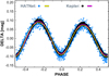 |
Fig. 1. Comparison of the folded light curves and the corresponding fourth-order Fourier fits (continuous lines) for the HATnet and Kepler observations on KIC 9832227. The adjacent datasets, corresponding to Tmid = 875 and 878 and the ephemeris used can be found in Table 1. To avoid crowding, every second data point is plotted. |
Times of the primary minima for KIC 9832227.
Throughout this work we use LCs obtained by simple ensemble photometry. For high-precision photometric time series analysis, application of filtering methods that clean up the data from colored noise play a crucial role in the full utilization of the signal content of the time series (see Kovacs et al. 2005; Tamuz et al. 2005; Bakos et al. 2010; Smith et al. 2012). There are several reasons for our decision to stay with the more standard photometric data stems. First, not all datasets contain these filtered LCs (e.g., ASAS-SN). Second, since the amplitude of the light variation is large compared to that of the colored noise, the application of these filtering methods should consider this fact, otherwise the filtered signals will be distorted (see Kovacs 2018). The systematics-filtered LCs, available at the download sites do not have a proper correction for this effect. Third, tests made with systematics-filtered LCs as given at the download sites (i.e., not containing the signal reconstruction feature listed in point 2 above) yield epochs within the error limits of the values derived from the ensemble photometric data.
To further boost the coverage of the period variation, we made a thorough search of other survey projects, including space missions. This search provided us with data sources from the infrared survey satellite WISE (Wright et al. 2010) through the ASAS-SN supernova search program (Shappee et al. 2014 and Kochanek et al. 2017) to the inventory of AAVSO. The detailed description of the datasets used is given in Appendix A.
In dividing the data into segments of appropriate length to avoid smearing of the O–C values due to long individual time bases, we inspected the datasets separately and made a decision case by case. As a result, the time bases vary by several factors from one dataset to the next. Because of excessive errors or improper phase coverage, although certain observations were available, they were not used (e.g., data from the Palomar Transient Factory project; see Rau et al. 2009 and Law et al. 2009). To the other extreme, for the Kepler data, we could use an almost daily time base, but it would not serve the purpose of the long-term study of our target. Nevertheless, it is worth noting that such a study certainly has relevance from our point of view, since it is indicative of the inherent O–C jitter likely attributed to stellar activity. The analysis made by Socia et al. (2018) shows that the rms of this physical scatter is about 1–2 min on a timescale of several tens of days. As a result, for the Kepler data we use segments of ∼80 d, and avoid mixing various quarters if they show visible zero point differences.
Modulation periods derived by various methods.
It is important to choose the proper method to find the optimum way to estimate the epochs of the primary minima. Because of the varying light curve, this task is not entirely trivial, even though the basic light variation, originating from the eclipses of this W UMa-type system is decomposable into a Fourier sum of only a few components. We followed a simple empirical approach to select the best method. From the five proposed methods we selected the one that yielded the smallest residual scatter for the few-parameter O–C model to be described in detail in Sect. 3. The following methods have been proposed (we also show the identifier of the O–C value corresponding to these methods as labeled in Table 1).
(a) Fourier fit I – OC1. Fourth-order Fourier fit to the entire phase-folded light curve (as given on a certain timebase) and search for the primary minimum by using the densely sampled synthetic light curve.
(b) Fourier fit II – OC2. The same as (a), but we search for the moment of the secondary eclipse and shift the value by half of the period. We recall that the secondary eclipses are in many cases deeper than the primary eclipses; therefore, it is not entirely a bold idea to use these events to predict the moments of the primary eclipse, with the assumption of circular binary orbit.
(c) Fourier fit I+II – OC3. A simple average of the O–C values obtained by (a) and (b).
(d) Template fit Ia – OC4. Use of a representative light curve as a template and a simple residual minimization on the full orbital phase by shifting this template relative to the target time series. If the template is properly chosen, the amount of shift will be characteristic of the overall shift of the light curve, perhaps depending to a lesser extent on the temporal change in its shape. The template is generated by the Fourier fits in running the minimum search by method (a).
(e) Template fit Ib – OC5. The same as (d), but the rms of the residual is only calculated in a restricted range of the phase of the primary minimum (in our case ±0.1 in units of the orbital period).
In the O–C estimates based on Fourier fits and in the calculation of the templates for methods (d) and (e), the individual time series X(i) are fitted with a low-order Fourier sum of
 (1)
(1)
where t0 = 2 454 953.949183 and P0 = 0.4579515. This ephemeris, given by Socia et al. (2018), ensures remaining compatible with the earlier investigations and yields a near zero O–C value at HJD = 2 455 000.0. After experimenting with the Fourier order, we found that m = 4 yields a good representation of all subsets, even those with modest or gapped coverage of their folded LCs (see Fig. 2).
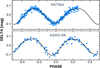 |
Fig. 2. Examples of the performance of the fourth-order Fourier fit (continuous line) for partially and sparsely covered cases. The light curves shown correspond to the datasets of Tmid = 998 and Tmid = 1840 as given in Table 1. |
For O–C values of type (d) and (e), we need to select a “proper” template that yields the best fit for our low parameter model with the O–C values derived with this favorable template. We present the test leading to our final choice in Sect. 3. Here we show only the Fourier fits to all 37 data segments analyzed in this paper and the three pre-selected candidates for the master template (see Fig. 3). To aid the template testing, specifically to have an overall view on the light curve morphology when selecting a subset of the light curves, the synthetic Fourier light curves have been ordered by the following algorithm.
 |
Fig. 3. Fourier-fitted synthetic light curves of all 37 data segments analyzed in this paper. The primary minima are shifted to zero phase. The time series are ordered on the basis of the closest neighbor, as described in Sect. 2. The pre-selected templates are shown by distinct colors. Following the notation of Table 1, the green, yellow, and magenta lines show the Fourier fits corresponding to segments Kepler-4, AAVSO-V-1, and AAVSO-V-4, respectively. |
Starting with any of the light curves with a serial index i ∈ [1, n], where n is the number of light curves (in our case 37), we find the closest neighbor to this light curve. This means that we search for the light curve yielding the smallest rms of the residuals obtained after subtracting the two time series from each other. We denote this rms between the ith test template and its nearest neighbor of serial index j as σ(i, j). Then, this closest neighbor is searched for its closest neighbor (excluding of course all the previously found close neighbors). We continue the search until the last closest neighbor is found. The mutual rms values {σ(i, k)} are examined and their variance is computed: 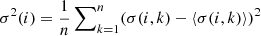 , where
  . The degree of smoothness of the ordering derived from the above search for the ith test template is then characterized by σ(i). We repeat this whole process for all possible starting templates. The smoothness parameters {σ(i)} for these orderings are examined, and the one with the lowest value is selected (with the associated starting template and ordering).
By using this algorithm we obtained the light curves shown in Fig. 3 with the set Kepler-4 as the starting template. It is clear that most of the light curves are very similar to each other, and that there are only four data segments that do not fit the overall smooth morphological sequence. These segments are AAVSO-V-2, WISE-W12, HAT-5, and WASP-1 (see the top four light curves in Fig. 3).
We summarize the datasets used and the O–C values derived in Table 1. The errors of the moments (eOC#) of the mid-eclipses were computed from a simple Monte Carlo test. In the case of the moments derived from Fourier fits for the given subset, the best-fit Fourier signal is perturbed by a realization of a Gaussian noise with the standard deviation obtained by the fit to the real data. Then this mock signal is fitted in the same way as the real data, and the moment of the mid-eclipse is stored. The process is repeated 1000 times and the standard deviation of the moments of these mid-eclipse values is considered as the error of the moment of the observed eclipse. For the eclipse times derived from template fitting the procedure is the same, except for the second step where, instead of fitting a Fourier sum to the mock signal, we use a template.
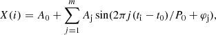
The O–C data presented in Table 1 are plotted in Fig. 4. It is worth emphasizing that 3σ error bars are used since standard 1σ bars would not be visible in most cases. We also note that former works by Molnar et al. (2017) and Socia et al. (2018) did not use the WASP segment near HJD − 2 455 000.0 = −2000, the HATNet, the ASAS-SN, the AAVSO, and the WISE data (but they used their own observations). The horizontal coordinate of each subset corresponds to the center of the time span of the given set. The horizontal bars are the half ranges of these time spans.
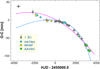 |
Fig. 4. Observed minus calculated moments of the primary minima for KIC 9832227 obtained via the template fit method yielding the OC4 values (see Sect. 2). The reference period and epoch of the primary eclipse are from Socia et al. (2018): P = 0.4579515 d, EPOCH = 2 454 953.949183 BJD. The light blue line shows the exponential model of Molnar et al. (2017) reaching singularity in 2022.2 (at HJD−2 455 000.0 = 4651). Shown is the best-fit parabola, assuming only a linear period decrease (magenta line). Data associated with certain surveys are highlighted; see Table 1 for the full dataset. |
We see that the Vulcan observations (second point from the left) and the HATNet and WASP data clearly breaks the exponential trend fitting based on data gathered after JD = 2 455 000.02. Furthermore, assuming a simple linear period change for the approximation of the overall parabolic trend also leads to an unsatisfactory fit (magenta line in Fig. 4). The smooth, non-monotonic deviations from these simple representations indicate that the observed O–C values require a more involved modeling.
3. Decomposition of the O–C variation
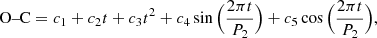
Due to the limited number of data points, we aimed for a modeling that is parsimonious (with respect of the number of parameters fitted) and at the same time physically sound. This lead to the obvious choice of decomposing the observed O–C values into components of a linear period decrease and a periodic variation, modeled simply with a sine function of arbitrary amplitude and phase
 (2)
(2)
where O–C is the observed timing difference in [min], t = HJD − 2 455 000.0, and P2 is the period of the sinusoidal component. The other possibility would be to continue with higher order polynomial representation. To test briefly the goodness of fit for the pure polynomial approximation, we used the OC4 data (see Table 1; the observed moments of minima were derived with the aid of template Kepler-4). Here, and throughout the paper, Eq. (2) is fitted by simple least squares technique with equal weights. For the fourth-order polynomial fit the unbiased rms of the fit was 2.83 min, exceeding significantly the fitting rms of 1.38 min of the polynomial plus sinusoidal model. We may get a similar rms of 1.46 min with the pure polynomial fit if we increase the order by one, but then the fit suggests a steep downward trend for dates less than −3600. A further increase of the polynomial order leads to overshooting in the empty part of the dataset, between −3600 and −2100. We see that there is a preference toward the data representation indicated by Eq. (2).
To determine the best period for the sinusoidal component, we scanned the period in the [4000, 8000] d interval and searched for the lowest residual scatter given by the least squares fit of Eq. (2). With the best period found, we followed the same type of simple Monte Carlo method to estimate the error of the period, as described in Sect. 2 for the calculation of the errors of the O–C values. Figure 5 shows the run of rms for the finally accepted method, using full phase-folded light curve fits by employing the set Kepler-4 as the template. Comparison with the other methods and templates is given in Table 2. We see that the full-phase template fit performs well, with some dependence on the template used. Based on these tests, we set the long-term modulation period P2 equal to (4925 ± 142) d.
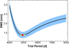 |
Fig. 5. Period scan of the O–C data obtained by the template fit method (see column OC4 of Table 1). Eq. (2) is used to find the minimum rms of the residuals (black line). Shown are the 1σ ranges of the residuals of the simple Monte Carlo simulations (shaded area) and the optimum period and its 1σ error from the above simulations (red dot and error bar). |
With the period known, we can decompose the data into a quadratic and a periodic part. The result is shown in Fig. 6. It seems that this simple model fits the data near the noise level expected from the physical jitter of the minima due to stellar activity (Socia et al. 2018) and from the overall statistical error due to observational noise.
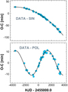 |
Fig. 6. Result of the joint fit of a second-order polynomial and a single sinusoidal to the data shown Fig. 4. The data plotted in the upper panel are free from the sinusoidal, whereas those shown in the lower panel from the polynomial component. See Table 3 for the regression coefficients of these components. |
Parameters of the polynomial plus sinusoidal fit.
The regression parameters and their standard errors are listed in Table 3. The errors are 1σ standard deviations and are derived directly from the inverse of the normal matrix. The error of the amplitude of the periodic component results from random simulations assuming independent Gaussian errors with standard deviations given on c4 and c5 from the inverse of the normal matrix. Figure 6 and the errors of the physically interesting quantities (period change Pdot and amplitude of the periodic component Ampl), together with the low residual scatter, indicate that the chosen mathematical representation is quite suitable for the description of the available data. For a sanity check of the solution above, in Appendix B we present the solution obtained by the Markov chain Monte Carlo (MCMC) method.
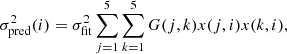
In spite of the good fit to the observations, the predictive power of the derived polynomial plus sinusoidal model is not very high. For a fixed period of the sinusoidal component we can give an estimate on the variance of the predicted O–C values for arbitrary moments by using the inverse of the normal matrix of the linear regression of Eq. (2),
 (3)
(3)
where σfit is the unbiased standard deviation of the residual of the regression, {G(j, k)} is the inverse of the normal matrix, and {x(j, i)} is the set of vectors associated with the jth regression coefficient cj (see Eq. (2)) at moment ti. Although the above formula is exact, it does not account for the error introduced by the period P2. To consider the contribution of the period estimation, we need to perform a Monte Carlo simulation. Here we use the synthetic data obtained by the fit to the original input time series with the best period. We add observational noise (Gaussian, with the standard deviation given by σfit) and then fit the data by Eq. (2), where P2 is also perturbed with a Gaussian error of σ = 142 (see Table 3). We repeat this process 500 times and arrive at the point-by-point standard deviations of the realization-dependent predicted O–C values. Figure 7 shows the resulting regions visited by the realizations, scaled by σpred. We note that using Eq. (3) (i.e., neglecting the effect of the P2 ambiguity), we get a somewhat more restricted prediction space, with a 3σ limit corresponding to the 2σ limit of the result shown. If the model is correct, in the following 3–4 years the periodic component will pass the minimum and will start to rise by a few minutes, which can be verified rather easily even by sporadic observations.
 |
Fig. 7. Polynomial plus sinusoidal fit (thick black line) of the observed O–C values (yellow dots, OC4 in Table 1). From darker to lighter shading, the blue regions show the 1, 2 and 3σ limits of the predicted O–C ranges, assuming errors in all estimated parameters, including P2, the period of the long-term variation. The inset shows the deviation from the best fit to the currently available data. |
4. Physical interpretation
First we discuss the possible physical causes giving rise to the periodic component of the O–C variation. There are be three possible causes of this type of variation: (i) change in the stellar structure due to stellar magnetic cycles (the so-called Applegate-effect; see Applegate 1992); (ii) apsidal motion mainly due to the finite size and non-spherical shape of the components (e.g., Mazeh 2008); (iii) light-time effect due to an external perturber (e.g., Wolf 2014).
For a brief check of possibility (i) we follow Almeida et al. (2019) and use the empirical studies of Oláh et al. (2009), Savanov (2012), and Vida et al. (2013, 2014) to see if our target follows the relation between the rotation frequency and the magnetic cycle length. We make the obviously non-stringent assumption that the orbital period is a good proxy of the rotation period. The result is shown in Fig. 8. Because our target has a rather small error bar even on the longer period, yielding σ(log(Plong/Prot)) ∼ 0.013, the outlier status of this object is quite likely, assuming that the observed trend also continues in the currently poorly explored parameter regime.
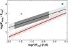 |
Fig. 8. Position of KIC 9832227 (light blue dot) on the schematic diagram relating the rotation frequency to the ratio of the period of the long-term cyclic luminosity variation due to stellar activity to the rotation period. The shaded area covers the data points shown by Almeida et al. (2019), based on the studies of Vida et al. (2013, 2014), Oláh et al. (2009), and Savanov (2012). Shown are red dwarfs (pink) and other stars (dark gray), with the extension to non-populated regions (light gray). Isolated small gray squares indicate objects distinct from the bulk of the sample. |
Possibility (ii) may occur due to the slow drift of the apsis line in systems with eccentric orbits. One of the characteristics of this phenomenon is the anticorrelation of the timings of the primary and secondary minima (e.g., Wolf et al. 2008). For our target, this explanation is also unlikely. First, the eccentricity must be very low, as suggested by the good fit of the radial velocity data with the assumption of zero eccentricity (see Molnar et al. 2017). Second, the difference between the primary and secondary O–C values (see Table 1) also supports the assumption of near-zero eccentricity. Leaving out the secondary eclipse outliers WISE-W12 and HAT-5, the average difference (ΔT = T2 − T1 − Porb/2) is −2.0 min with a standard deviation of 2.7 min for the remaining 37 points. This implies  (see, e.g., Winn 2010), where the error was estimated from the error of the average ΔT. Third, the period of the sinusoidal component of the O–C variation of our target is relatively short, and therefore not too common among objects showing apsidal motion (see Hong et al. 2016 and Zasche et al. 2018).
Possibility (iii) implies that the system is a hierarchical triplet, with an outer component on a 4925 d orbit. The mass function can be estimated from the amplitude of the sinusoidal component of the total O–C variation. With the assumption of zero eccentricity, this yields: M3 ≥ (0.38 ± 0.02) M⊙, where the error is the standard deviation of the values obtained by including the Gaussian errors of all constituent parameters. We recall that this mass (although it is a lower limit) is still allowed by the test performed on the composite spectral broadening function by Molnar et al. (2017). They suggest an upper limit of 0.5 M⊙ for any possible third component, assuming that it is a main sequence star.
Although it is not expected that the third star with its low luminosity (implied by its mass) will give any appreciable contribution to the total spectral energy distribution (SED) of the system, it is still useful to check the actual values and explore the effect of components different from a main sequence star. We gathered 18 wide-band color values from the near ultraviolet to infrared regime. After converting all magnitudes to the Vega system, we compared these values by the theoretical SEDs obtained from various stellar atmosphere models (we refer to Appendix C for additional details on the data and the models). The final SED values are plotted in Fig. 9.
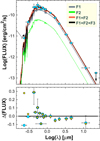 |
Fig. 9. Comparison of the observed and theoretical SEDs for KIC 9832227. Dots denote observed values, with 3σ vertical error bars, and equivalent waveband widths (horizontal bars). The inset shows the various theoretical SEDs: F1 – primary only, F2 – secondary only, F1+F2 – binary only, F1+F2+F3 – binary with a hypothetical third component (K/M dwarf or white dwarf; black lines, which differ only in the UV). Lower panel: residual in respect of the three-component solution: blue dots – white dwarf, yellow dots – K/M dwarf for the third component. The stellar atmosphere models of Castelli et al. (1997) and Koester (2010) are used (see text and Appendix C for more details). |
Assuming that the third component is a main sequence star (a late K dwarf or an early M dwarf) we set its radius equal to 0.4 R⊙. For the binary we used the parameters of Molnar et al. (2017) and the Gaia distance (585 ± 10 pc) to derive the observable fluxes from the stellar atmosphere model fluxes. As presented in Fig. 9, with the main sequence assumption, we cannot get any additional support for the existence of the third component. Furthermore, we note that the analysis of the near-IR spectra made by the NASA Infra-Red Telescope Facility by Pavlenko et al. (2018) also did not show any obvious sign of the presence of a third component.
On the other hand, we see that the Galex near-UV (NUV) flux at the far left is significantly above the model flux. This observation led us to test the possibility of another third body scenario, by assuming that it is a relatively low-mass white dwarf (WD). We see that adding the flux of a Teff = 30 000 K, R = 0.016 R⊙ WD almost fixes the discrepant position of the NUV flux, but leaves the overall fine match at all other wavelengths. Nevertheless, the scatter at the peak SED regime is still somewhat high, likely because of the larger observational errors of some of the fluxes; the flux variations due to eclipses are rather small, and some fluxes result from averaging several observations spread through many orbital periods. For instance, the outlier status of the GaiaG-band is hard to understand at this moment because it is surely not due to some single measurement or bad phase effect. In addition to the scatter, an upward trend toward shorter wavelengths near the peak flux is also observable. This is a sign of the overestimation of the reddening. As discussed in Appendix C, the reddening value of E(B − V) = 0.082 based on the map of Schlafly & Finkbeiner (2011) is more than a factor of two higher than the value derived by Molnar et al. (2017) from the combination of spectroscopic and photometric data. With E(B − V) = 0.03 we can eliminate the trend and considerably lower the likelihood of the WD scenario, but we cannot cure the scatter around the maximum flux.
Concerning the monotonic component of the total period variation, it is interesting to compare the rate of period change with those observed in other binaries. As a basis of comparison, we selected the recent analysis of 22 500 binaries in the Galactic Bulge by Pietrukowicz et al. (2017). Figure 10 shows that the rate of period change of KIC 9832227 is quite similar to most of the stars analyzed in the above work. Indeed, V1309 Sco, the only verified nova precursor (Tylenda et al. 2011) clearly stands out with its dramatic period decrease from the other normal binaries. Although there is an excess of systems with higher negative period change, the nearly equal number of systems with positive and negative period changes (52 and 56, respectively) indicates that the cause of most of the period changes lies in some temporal (long-term) variation rather than an inward spiraling of the components. One possibility is the presence of distant perturbers with substantially longer period than the time span of the data. In the analysis performed by Pietrukowicz et al. (2017), the time base extends from 1997 to 2015, and in some cases from 1992 depending on the availability of data from the various OGLE phases. Even though this 20–25 year time span is quite remarkable, there are several examples of systems with tertiary components of even longer periods (see, e.g., Sarotsakulchai et al. 2019 and Tokovinin 2014, for a review). We also recall that Pietrukowicz et al. (2017) identified also 35 binaries with cyclic O–C variations. The high number of cyclic period changers is further supported by the current survey of the same area by Hajdu et al. (2019), using all available data from the OGLE-IV archive. From the 80 000 systems examined, they found 992 with cyclic O–C variations. We conclude that in the specific case of KIC 9832227 the total time span of the data used in this investigation is ∼19 years, which leaves still enough room for the fourth-body interpretation of the apparent linear period change. At the same time, continuation of the monotonic variation of the period is also a possibility. This may come from various sources, such as mass transfer within the W UMa components, angular momentum loss due to magnetic wind (e.g., Yang & Liu 2003; Toonen et al. 2016). The complex nature of these processes do not allow a more detailed study of these possibilities within the limitation of this work.
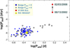 |
Fig. 10. Comparison of the size of the observed period changes of various groups of binaries. The verified pre-nova V1309 Sco stands out thanks to its huge rate and its change during six years of observations. Instead, KIC 9832227 lies in the middle of the binaries and shows a significant but relatively low negative period change in the Galactic Bulge sample of Pietrukowicz et al. (2017). For comparison, also plotted are the stars from the above survey, showing period increase. |
5. Conclusions
The work by Socia et al. (2018) on the negation of the nova candidate status of KIC 9832227 stimulated our deeper investigation of this W UMa-type binary system. Because the conclusion of Socia et al. (2018) rests mainly on the misidentification of a single early epoch, we thought that the period variation should be further investigated by using additional data available from various ground- and space-based instruments. Thanks to the wide-field survey HATNet and to the renewed analysis of the WASP survey, we successfully built up a crucial early period of the O–C variation. In addition to the already utilized public domain data by Molnar et al. (2017) and Socia et al. (2018) we also found extremely useful data from the supernova survey ASAS-SN, from AAVSO, and from the WISE satellite. The 39 epochs were accurate enough to clearly decompose the period variation into a linear and a sinusoidal part. We found that the linear rate of change is equal to ( − 1.097 ± 0.047) × 10−6 d yr−1. This value fits in the overall rate observed in many binary systems. The period and the amplitude of the sinusoidal components are equal to (4925 ± 142) d and (10.98 ± 0.37) min. We found that the most plausible explanation for the source of this variation is the light-time effect of an outer perturber. The estimated lower limit of the mass of the outer companion is (0.38 ± 0.02) M⊙. This value, assuming that the third component is a main sequence star, is below the upper mass limit allowed by the non-detection of the corresponding feature in the broadening function analysis of Molnar et al. (2017). With the significant deviation of the GALEX NUV point from the composite SED constructed under the assumption of a main sequence tertiary, we also tested the replacement of this component with a white dwarf. We found a better fit, but the contribution of the white dwarf component induces a large UV excess at shorter wavelengths. Currently, there are no data available at these short wavelengths, but future observations might easily confirm or negate the viability of the white dwarf scenario. A further ambiguity in the white dwarf hypothesis is the poorly known value of the reddening. Using E(B − V) = 0.03 (i.e., more than a factor of two lower than the one employed in this paper) decreases the probability of a white dwarf companion considerably.
The point from the NSVS archive also supports this trend. However, as pointed out by Socia et al. (2018), this suffered from an MJD/HJD ambiguity in the work of Molnar et al. (2017) that yielded the apparent confirmation of the exponential trend.
For Gaia, see the VizieR site, for WISE, see: http://wise2.ipac.caltech.edu/docs/release/allwise/faq.html
Acknowledgments
We thank Sebastian Otero at AAVSO for answering our questions on various aspects of the data accessed. We are grateful to the observers listed in Appendix A of this paper for their valuable contribution via the AAVSO database. We acknowledge the improvement in the model fit by following the suggestion of the referee of using uniform timebase (i.e., BJD) for all data. Thanks are due also to Yakiv Pavlenko, for the correspondence on the analysis of the NIR spectra. This research has made use of the International Variable Star Index (VSX) database operated at AAVSO, Cambridge, Massachusetts, USA. This paper includes data collected by the Kepler mission. Funding for the Kepler mission is provided by the NASA Science Mission directorate. This publication makes use of data products from the Wide-field Infrared Survey Explorer, which is a joint project of the University of California, Los Angeles, and the Jet Propulsion Laboratory/California Institute of Technology, funded by the National Aeronautics and Space Administration. The NSVS data have been downloaded from the site of SkyDOT, operated by the University of California for the National Nuclear Security Administration of the US Department of Energy. This research has made use of the VizieR catalogue access tool, CDS, Strasbourg, France (DOI: 10.26093/cds/vizier). Support from the National Research, Development and Innovation Office (grants K 129249 and NN 129075) are acknowledged. Data presented in this paper are based on observations obtained by the HAT station at the Submillimeter Array of SAO, and the HAT station at the Fred Lawrence Whipple Observatory of SAO. HATNet observations have been funded by NASA grants NNG04GN74G and NNX13AJ15G.
Note added in proof. While preparing the associated CDS material, we recognized that not all of the data segments had been selected from the time series based on the ensemble photometry channel of the HATNet pipeline, as stated in the text. Some data segments used the time series produced via the method of external parameter decorrelation by Bakos et al. (2010). Please consult the accompanying README file from the CDS material for more detailed information.
References
- Abbott, B. P., Abbott, R., Abbott, T. D., et al. 2016, Phys. Rev. Lett., 116, 061102 [Google Scholar]
- Almeida, L. A., de Almeida, L., Damineli, A., et al. 2019, AJ, 157, 150 [NASA ADS] [CrossRef] [PubMed] [Google Scholar]
- Apellaniz, J. M., & Gonzalez, M. P. 2018, A&A, 616, L7 [NASA ADS] [CrossRef] [EDP Sciences] [Google Scholar]
- Applegate, J. H. 1992, ApJ, 385, 621 [NASA ADS] [CrossRef] [Google Scholar]
- Bakos, G., Noyes, R. W., Kovács, G., et al. 2004, PASP, 116, 266 [NASA ADS] [CrossRef] [Google Scholar]
- Bakos, G. Á., Torres, G., Pál, A., et al. 2010, ApJ, 710, 1724 [NASA ADS] [CrossRef] [Google Scholar]
- Borucki, W. J., Caldwell, D., Koch, D. G., et al. 2001, PASP, 113, 439 [NASA ADS] [CrossRef] [Google Scholar]
- Borucki, W. J., Koch, D., Basri, G., et al. 2010, Science, 327, 977 [NASA ADS] [CrossRef] [PubMed] [Google Scholar]
- Bovy, J., Rix, H.-W., Green, G. M., et al. 2016, ApJ, 818, 130 [NASA ADS] [CrossRef] [Google Scholar]
- Castelli, F., Gratton, R. G., & Kurucz, R. L. 1997, A&A, 318, 841 [NASA ADS] [Google Scholar]
- Davenport, J. R. A., Ivezic, Z., Becker, A. C., et al. 2014, MNRAS, 440, 3430 [NASA ADS] [CrossRef] [Google Scholar]
- Ferreira, T., Saito, R. K., Minniti, D., et al. 2019, MNRAS, 486, 1220 [NASA ADS] [CrossRef] [Google Scholar]
- Frei, Z. S., & Gunn, J. E. 1994, AJ, 108, 1476 [NASA ADS] [CrossRef] [Google Scholar]
- Hajdu, T., Borkovits, T., Forgács-Dajka, E., et al. 2019, MNRAS, 485, 2562 [NASA ADS] [CrossRef] [Google Scholar]
- Hong, K., Lee, J. W., Seung-Lee Kim, S.-L., et al. 2016, MNRAS, 460, 650 [NASA ADS] [CrossRef] [Google Scholar]
- Kirk, B., Kyle Conroy, K., Prsa, A., et al. 2016, AJ, 151, 68 [NASA ADS] [CrossRef] [Google Scholar]
- Kochanek, C. S., Shappee, B. J., Stanek, K. Z., et al. 2017, PASP, 129, 104502 [NASA ADS] [CrossRef] [Google Scholar]
- Koester, D. 2010, Mem. Soc. Astron. It., 81, 921 [NASA ADS] [Google Scholar]
- Kovacs, G. 2018, A&A, 614, L4 [NASA ADS] [CrossRef] [EDP Sciences] [Google Scholar]
- Kovacs, G., Bakos, G., & Noyes, R. W. 2005, MNRAS, 356, 557 [NASA ADS] [CrossRef] [Google Scholar]
- Kuncarayakti, H. 2016, J. Phys.: Conf. Ser., 728, 072019 [CrossRef] [Google Scholar]
- Law, N. M., Kulkarni, S. R., Dekany, R. G., et al. 2009, PASP, 121, 1395 [NASA ADS] [CrossRef] [Google Scholar]
- Liu, T., & Janes, K. A. 1990, ApJ, 354, 273 [NASA ADS] [CrossRef] [Google Scholar]
- Mason, E., Diaz, M., & Williams, R. E. 2010, A&A, 516, A108 [NASA ADS] [CrossRef] [EDP Sciences] [Google Scholar]
- Mazeh, T. 2008, EAS Publ. Ser., 29, 1 [CrossRef] [Google Scholar]
- McCall, M. L. 2004, AJ, 128, 2144 [NASA ADS] [CrossRef] [Google Scholar]
- Molnar, L. A., van Noord, D. M., Kinemuchi, K., et al. 2017, ApJ, 840, 1 [NASA ADS] [CrossRef] [Google Scholar]
- Nakano, S., Nishiyama, K., & Kabashima, F. 2008, IAU Circ., 8972 [Google Scholar]
- Oláh, K., Kolláth, Z., Granzer, T., et al. 2009, A&A, 501, 703 [NASA ADS] [CrossRef] [EDP Sciences] [Google Scholar]
- Pastorello, A., Mason, E., Taubenberger, S., et al. 2019, A&A, 630, A75 [NASA ADS] [CrossRef] [EDP Sciences] [Google Scholar]
- Pavlenko, Y. A. V., Evans, A., Banerjee, D. P. K., et al. 2018, A&A, 615, A120 [NASA ADS] [CrossRef] [EDP Sciences] [Google Scholar]
- Pejcha, O., Metzger, B. D., Tyles, J. G., et al. 2017, ApJ, 850, 59 [NASA ADS] [CrossRef] [Google Scholar]
- Pietrukowicz, P., Soszyński, I., Udalski, A., et al. 2017, Acta Astron., 67, 115 [NASA ADS] [Google Scholar]
- Pollacco, D. L., Skillen, I., Collier Cameron, A., et al. 2006, PASP, 118, 1407 [NASA ADS] [CrossRef] [Google Scholar]
- Podsiadlowski, P., Joss, P. C., Hsu, J. J. L., et al. 1992, ApJ, 391, 246 [NASA ADS] [CrossRef] [Google Scholar]
- Pojmanski, G., Pilecki, B., & Szczygiel, D. 2005, Acta Astron., 55, 275 [NASA ADS] [Google Scholar]
- Rau, A., Kulkarni, S. R., Law, N. M., et al. 2009, PASP, 121, 1334 [NASA ADS] [CrossRef] [Google Scholar]
- Romero, A. D., Kepler, S. O., Joyce, S. R. G., et al. 2019, MNRAS, 484, 2711 [NASA ADS] [Google Scholar]
- Sanders, J. L., & Das, P. 2018, MNRAS, 481, 4093 [NASA ADS] [CrossRef] [Google Scholar]
- Sarotsakulchai, T., Qian, S.-B., Soonthornthum, B., et al. 2019, PASJ, 71, 81 [NASA ADS] [CrossRef] [Google Scholar]
- Savanov, I. S. 2012, Astron. Rep., 56, 716 [NASA ADS] [CrossRef] [Google Scholar]
- Schlafly, E. F., & Finkbeiner, D. P. 2011, ApJ, 737, 103 [NASA ADS] [CrossRef] [Google Scholar]
- Shappee, B. J., Prieto, J. L., Grupe, D., et al. 2014, ApJ, 788, 48 [NASA ADS] [CrossRef] [Google Scholar]
- Smith, J. C., Stumpe, M. C., Van Cleve, J. E., et al. 2012, PASP, 124, 1000 [NASA ADS] [CrossRef] [Google Scholar]
- Socia, Q. J., Welsh, W. F., Short, D. R., et al. 2018, ApJ, 864, L32 [NASA ADS] [CrossRef] [Google Scholar]
- Tamuz, O., Mazeh, T., & Zucker, S. 2005, MNRAS, 356, 1466 [NASA ADS] [CrossRef] [Google Scholar]
- Ter Braak, C. J. F. 2006, Stat. Comput., 16, 239 [Google Scholar]
- Tokovinin, A. 2014, AJ, 147, 87 [NASA ADS] [CrossRef] [Google Scholar]
- Toonen, S., Hamers, A., & Portegies, Z. S. 2016, Comput. Astrophys. Cosmol., 3, 36 [NASA ADS] [CrossRef] [Google Scholar]
- Truran, J. W., & Cameron, A. G. W. 1971, Ap&SS, 14, 179 [NASA ADS] [CrossRef] [Google Scholar]
- Tylenda, R., Hajduk, M., Kamiński, T., et al. 2011, A&A, 528, A114 [NASA ADS] [CrossRef] [EDP Sciences] [Google Scholar]
- Vida, K., Kriskovics, L., & Oláh, K. 2013, AN, 334, 972 [NASA ADS] [CrossRef] [Google Scholar]
- Vida, K., Oláh, K., & Szabó, R. 2014, MNRAS, 441, 2744 [NASA ADS] [CrossRef] [Google Scholar]
- Wang, S., & Chen, X. 2019, ApJ, 877, 116 [NASA ADS] [CrossRef] [Google Scholar]
- Winn, J. N. 2010, ArXiv e-prints [arXiv:1001.2010v5] [Google Scholar]
- Wolf, M. 2014, Contrib. Astron. Obs. Skalnate Pleso, 43, 493 [NASA ADS] [Google Scholar]
- Wolf, M., Zejda, M., & de Villiers, S. N. 2008, MNRAS, 388, 1836 [NASA ADS] [CrossRef] [Google Scholar]
- Woźniak, P. R., Vestrand, W. T., Akerlof, C. W., et al. 2004, AJ, 127, 2436 [NASA ADS] [CrossRef] [Google Scholar]
- Wright, E. L., Eisenhardt, P. R. M., Mainzer, A. K., et al. 2010, AJ, 140, 1868 [NASA ADS] [CrossRef] [Google Scholar]
- Yang, Y., & Liu, Q. 2003, PASP, 115, 748 [NASA ADS] [CrossRef] [Google Scholar]
- Yuan, H. B., Liu, X. W., & Xiang, M. S. 2013, MNRAS, 430, 2188 [NASA ADS] [CrossRef] [Google Scholar]
- Zasche, P., Wolf, M., Uhlar, R., et al. 2018, A&A, 619, A85 [NASA ADS] [CrossRef] [EDP Sciences] [Google Scholar]
Appendix A: Data sources and data handling
Here we describe some relevant pieces of information concerning the data used in the O–C analysis and displayed in Table 1. First, we note that the values for the Vulcan and MLO data are from Socia et al. (2018) (as a result, all OC values are the same for these items). In the case of the AAVSO data, we used only V and I observations because the other colors did not have proper phase coverage. The web sites and the appropriate journal references for the data sources are as follows:
-
AAVSO: https://www.aavso.org/vsx/
-
ASAS: http://www.astrouw.edu.pl/asas/ Pojmanski et al. (2005) and references therein
-
ASAS-SN: https://asas-sn.osu.edu/ Shappee et al. (2014) and Kochanek et al. (2017)
-
Kepler: http://keplerebs.villanova.edu/ Borucki et al. (2010) and Kirk et al. (2016)
-
NSVS: https://skydot.lanl.gov/nsvs/nsvs.php Woźniak et al. (2004)
The HATNet data are publicly accessible3. The data used in this paper are accessible through the CDS. These data result from an early reduction, and therefore might be slightly different from the data included in the full public HAT archive. Nevertheless, the possible differences are expected to have only a small effect on the O–C values.
Following the notation of Table 1, the notes below are relevant from the point of view of the analysis presented in this paper (see also some related notes in Sect. 2).
AAVSO-V-1 – AAVSO-V-5. Because the data were gathered by different observers with different instruments, they are often not on the same zero point. In addition, not all the data are of the same quality. If necessary we adjusted the quality requirement to the goal of segmental sampling by entirely omitting observations owned by a given observer. By using the observer assignment code of AAVSO data site, we broke down the V data in the following way: AAVSO-V-1: observer PVEA (Velimir Popov); AAVSO-V-2: observers SAH (Gerard Samolyk), RIZ (John Ritzel) and TRE (Ray Tomlin) with a zero point shift applied only to SAH; AAVSO-V-3: observers CDSA (David Conner), HJW (John Hall), DUBF (Franky Dubois), and TRE, ZP(CDSA) = +0.037, and all other zero point shifts are zero; AAVSO-V-4: observers KTU (Timo Kantola), HJW and TRE and ZP(KTU) = −0.04; ZP(HJW) = −0.025; AAVSO-V-5: observers TRE, SAH, SNE (Neil Simmons), and DUBF, with ZP(SAH) = +0.019, and all other zero point shifts are zero.
AAVSO-I-1. The data from DUBF and TRE are used, with ZP(DUBF) = − 0.0092.
ASAS-IV. Because the data suffer from relative high observational noise, the observations made in I and V colors have been merged with a zero point shift of +0.717 for the I data. We selected “grade A” data from the V observations and averaged the magnitudes in Cols. 2–5, corresponding to different aperture sizes. For the I data the “grade A” selection resulted in only five data points. Therefore, we used all data points and averaged only Cols. 4 and 5.
ASAS-SN-1 – ASAS-SN-4. The data quality and the number of data points allowed us to separate the full dataset into four segments.
HAT-1 – HAT-5. To avoid possible signal suppression when the data are corrected for instrumental systematics (but not reconstructed using the full signal+systematics model), we used the magnitudes derived from an ensemble photometry based on aperture fluxes. Because of the large field of view, the ensemble value of the stars observed during each exposure depends on the chip position (e.g., vignetting causes large changes in the stellar fluxes). From the three aperture sizes we selected the one that resulted in the smallest scatter of the folded light curve. Although dataset 4 is already compact in its entirety, it was divided into two parts because the large number of data points allowed us to do so, and thereby effects of short-term light curve changes can be assessed.
Kepler-1 – Kepler-15. The data quality and the number of data points allowed us to separate the full dataset into 15 segments with ∼3500 data points in each segment. We avoided including different Quarters in the same data segment if zero point differences were obvious. Similarly to the HAT data, the simple aperture flux (Col. 3) is used.
NSVS-12. We employed the data acquired by the two cameras observing the field that hosts KIC 9832227. As in other cases, the moments of observations have been transformed to BJD (in this particular case, from MJD). A zero point correction of 0.060 mag is also applied to the dataset acquired by one of the cameras.
WASP-1, WASP-3, WASP-4. Unfortunately, we had to leave out WASP-2, because of the bad phase coverage of the data points for this dataset between HJD 2 453 901.662 and 2 453 952.427.
WISE-W12. This is a merged set of the data gathered in the W1 and W2 filters. The data were taken in two campaigns, separated by a gap of half a year. There is a zero point shift of ∼0.03 mag between the two segments. A closer examination shows that the data from the two bands also have zero point differences on the order of ∼0.01 mag, depending on which of the two campaigns is considered. By performing these campaign- and filter-dependent shifts, we ended up with a time series containing 116 items. In spite of the above adjustments, the data still show significant scatter of 0.028 mag around a fourth-order Fourier fit. Nevertheless, the accuracy of the O–C value is still acceptable for our purpose.
Appendix B: The MCMC solution
In finding the best-fit solution for Eq. (2) to the O–C data in Table 1 (labeled OC4), we performed a differential evolution Markov chain Monte Carlo (DEMCMC) analysis following Ter Braak (2006). We assumed uniform priors on all of the parameters given in Eq. (2). Additionally, we introduced a parameter to account for excess scatter in the O–C values above the estimated uncertainties. This scatter was added in quadrature to all of the listed errors, and was allowed to vary in the analysis using a uniform logarithmic prior.
The resulting parameter–parameter plots are shown in Fig. B.1. In most cases the cross-correlation effect is not substantial, at least in the close neighborhood of the high-density/low-χ2 regimes that determine the most probable solution. We list the final parameters with their 1σ errors in Table B.1. In comparing the solution derived from the standard least squares fit (see Table 3), we see a good agreement for the parameter values. However, the MCMC errors are larger because they include the effect of the various choices of all other parameters, whereas in our least squares solution the period was fixed to its optimum value.
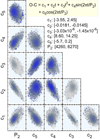 |
Fig. B.1. Diagnostic diagram based on the MCMC solution of the fit of the polynomial plus sinusoidal model (see inset) of the observed O–C values (see Table 1). Dots are color-coded according to the χ2 values: blue dots have the lowest χ2, whereas the gray dots (from dark to light) are associated with the less probable solutions. The parameter ranges of the plots are given in the inset. |
Best-fit parameters of the polynomial plus sinusoidal model by MCMC.
Appendix C: SED constituents
The magnitudes measured for KIC 9832227 are from the VizieR4 site. All magnitudes have been transformed to the Vega system by using the filter zero points, as given by the Spanish Visual Observatory5. To derive dereddened magnitudes, we accepted the reddening given by the map of Schlafly & Finkbeiner (2011) and accessible at the NASA/IPAC Infrared Science Archive6. This yields E(B − V) = 0.082 ± 0.002. Extinction in any given waveband was computed by Aλ = RλE(B − V), where the extinction coefficients Rλ given by Yuan et al. (2013), Sanders & Das (2018), Liu & Janes (1990), and Davenport et al. (2014) were used. For the XMM-Newton UVW1 band, we employed the York Extinction Solver7 (see McCall 2004). All the input data used to construct the observed SED for KIC 9832227 (see Fig. 9) are listed in Table C.1.
Observed magnitudes of KIC 9832227.
We note that the reddening value for KIC 9832227 is far from accurate, in spite of the small formal error bar of the value we used. Molnar et al. (2017) compare the spectroscopic and color-calibrated Teff values to derive a considerably lower value of E(B − V) = 0.030 ± 0.002. The MWDust tool by Bovy et al. (2016) yields E(B − V) = 0.021. Exceeding all these values, by using the extinction coefficients of Wang & Chen (2019), the Gaia catalog yields E(B − V) = 0.291 or 0.318 for the 68% lower limits, depending on whether we use their E(BP − RP) or AG values. Although these high values are clearly incompatible with the SED based on the accurate distance of the system, it is unclear whether some considerably lower value than the one we adopted is strongly justifiable by the present data.
Transformation to the Vega system was performed in the following way. When the observed magnitudes were given in the AB system (i.e., for GALEX, XMM, M 17), we computed m(Vega) = m(AB)+2.5log(ZP/3631), where the zero point ZP for the given waveband was taken from the Spanish Visual Observatory site. The Gaia and the WISE magnitudes are defined on the Vega system8, so their observed and transformed values are the same. The APASS magnitudes are in the Johnson system, which can be transformed to the AB system based on Frei & Gunn (1994) 9. Then these magnitudes were transformed to the Vega system, as mentioned above. The 2MASS magnitudes are nearly on the Vega system, but according to Apellaniz & Gonzalez (2018) there might be some systematic differences yielding the following shifts to the published values: J(Vega) = J(publ)−0.025 ± 0.005, H(Vega) = H(publ)+0.004 ± 0.005, and K(Vega) = K(publ)−0.015 ± 0.005. We applied these corrections to the observed 2MASS magnitudes.
The theoretical SEDs were downloaded from the Spanish Visual Observatory site10, using the grid closest to the observed parameters. For the binary components we used the Teff = 6000 K and 5750 K models, both with solar composition, logg = 4.0, and mixing length and microturbulence velocity of 1.25 and 2 km s−1, respectively. These models are without convective overshooting (see Castelli et al. 1997). The current Gaia distance of 585 ± 10 pc and the radii of Molnar et al. (2017) (1.58 R⊙ and 0.83 R⊙ for the primary and secondary component, respectively) were used to compute the predicted fluxes. In one scenario, the third component was assumed to be a Teff = 3500 K, R = 0.4 R⊙ main sequence star, whereas in another scenario it was assumed to be a white dwarf with Teff = 30 000 K, logg = 8.0, and R = 0.016 R⊙. In the latter scenario, we used the stellar atmosphere models of Koester (2010) downloaded from the site cited above. The parameters for the white dwarf model are broadly consistent with the model values of Romero et al. (2019) at the temperature chosen, and assuming a mass of M ∼ 0.49 M⊙. This stellar mass is above by 0.11 M⊙ of our minimum value derived from the light-time effect (see Sect. 4).
All Tables
All Figures
|
Fig. 1. Comparison of the folded light curves and the corresponding fourth-order Fourier fits (continuous lines) for the HATnet and Kepler observations on KIC 9832227. The adjacent datasets, corresponding to Tmid = 875 and 878 and the ephemeris used can be found in Table 1. To avoid crowding, every second data point is plotted. |
| In the text | |
|
Fig. 2. Examples of the performance of the fourth-order Fourier fit (continuous line) for partially and sparsely covered cases. The light curves shown correspond to the datasets of Tmid = 998 and Tmid = 1840 as given in Table 1. |
| In the text | |
|
Fig. 3. Fourier-fitted synthetic light curves of all 37 data segments analyzed in this paper. The primary minima are shifted to zero phase. The time series are ordered on the basis of the closest neighbor, as described in Sect. 2. The pre-selected templates are shown by distinct colors. Following the notation of Table 1, the green, yellow, and magenta lines show the Fourier fits corresponding to segments Kepler-4, AAVSO-V-1, and AAVSO-V-4, respectively. |
| In the text | |
|
Fig. 4. Observed minus calculated moments of the primary minima for KIC 9832227 obtained via the template fit method yielding the OC4 values (see Sect. 2). The reference period and epoch of the primary eclipse are from Socia et al. (2018): P = 0.4579515 d, EPOCH = 2 454 953.949183 BJD. The light blue line shows the exponential model of Molnar et al. (2017) reaching singularity in 2022.2 (at HJD−2 455 000.0 = 4651). Shown is the best-fit parabola, assuming only a linear period decrease (magenta line). Data associated with certain surveys are highlighted; see Table 1 for the full dataset. |
| In the text | |
|
Fig. 5. Period scan of the O–C data obtained by the template fit method (see column OC4 of Table 1). Eq. (2) is used to find the minimum rms of the residuals (black line). Shown are the 1σ ranges of the residuals of the simple Monte Carlo simulations (shaded area) and the optimum period and its 1σ error from the above simulations (red dot and error bar). |
| In the text | |
|
Fig. 6. Result of the joint fit of a second-order polynomial and a single sinusoidal to the data shown Fig. 4. The data plotted in the upper panel are free from the sinusoidal, whereas those shown in the lower panel from the polynomial component. See Table 3 for the regression coefficients of these components. |
| In the text | |
|
Fig. 7. Polynomial plus sinusoidal fit (thick black line) of the observed O–C values (yellow dots, OC4 in Table 1). From darker to lighter shading, the blue regions show the 1, 2 and 3σ limits of the predicted O–C ranges, assuming errors in all estimated parameters, including P2, the period of the long-term variation. The inset shows the deviation from the best fit to the currently available data. |
| In the text | |
|
Fig. 8. Position of KIC 9832227 (light blue dot) on the schematic diagram relating the rotation frequency to the ratio of the period of the long-term cyclic luminosity variation due to stellar activity to the rotation period. The shaded area covers the data points shown by Almeida et al. (2019), based on the studies of Vida et al. (2013, 2014), Oláh et al. (2009), and Savanov (2012). Shown are red dwarfs (pink) and other stars (dark gray), with the extension to non-populated regions (light gray). Isolated small gray squares indicate objects distinct from the bulk of the sample. |
| In the text | |
|
Fig. 9. Comparison of the observed and theoretical SEDs for KIC 9832227. Dots denote observed values, with 3σ vertical error bars, and equivalent waveband widths (horizontal bars). The inset shows the various theoretical SEDs: F1 – primary only, F2 – secondary only, F1+F2 – binary only, F1+F2+F3 – binary with a hypothetical third component (K/M dwarf or white dwarf; black lines, which differ only in the UV). Lower panel: residual in respect of the three-component solution: blue dots – white dwarf, yellow dots – K/M dwarf for the third component. The stellar atmosphere models of Castelli et al. (1997) and Koester (2010) are used (see text and Appendix C for more details). |
| In the text | |
|
Fig. 10. Comparison of the size of the observed period changes of various groups of binaries. The verified pre-nova V1309 Sco stands out thanks to its huge rate and its change during six years of observations. Instead, KIC 9832227 lies in the middle of the binaries and shows a significant but relatively low negative period change in the Galactic Bulge sample of Pietrukowicz et al. (2017). For comparison, also plotted are the stars from the above survey, showing period increase. |
| In the text | |
|
Fig. B.1. Diagnostic diagram based on the MCMC solution of the fit of the polynomial plus sinusoidal model (see inset) of the observed O–C values (see Table 1). Dots are color-coded according to the χ2 values: blue dots have the lowest χ2, whereas the gray dots (from dark to light) are associated with the less probable solutions. The parameter ranges of the plots are given in the inset. |
| In the text | |
Current usage metrics show cumulative count of Article Views (full-text article views including HTML views, PDF and ePub downloads, according to the available data) and Abstracts Views on Vision4Press platform.
Data correspond to usage on the plateform after 2015. The current usage metrics is available 48-96 hours after online publication and is updated daily on week days.
Initial download of the metrics may take a while.