| Issue |
A&A
Volume 631, November 2019
|
|
|---|---|---|
| Article Number | A80 | |
| Number of page(s) | 28 | |
| Section | Stellar atmospheres | |
| DOI | https://doi.org/10.1051/0004-6361/201935811 | |
| Published online | 23 October 2019 | |
Observational constraints on the origin of the elements
I. 3D NLTE formation of Mn lines in late-type stars★,★★
1
Max Planck Institute for Astronomy,
69117
Heidelberg,
Germany
e-mail: bergemann@mpia-hd.mpg.de
2
Ruprecht-Karls-Universität,
Grabengasse 1,
69117
Heidelberg,
Germany
3
Department of Physics, Western Michigan University,
Kalamazoo,
Michigan
49008,
USA
4
Stellar Astrophysics Centre, Department of Physics and Astronomy, Aarhus University,
8000
Aarhus C,
Denmark
5
Department of Theoretical Physics and Astronomy, Herzen University,
St. Petersburg
191186,
Russia
6
Montessori-Schule Dachau,
Geschwister-Scholl-Str. 2,
85221
Dachau,
Germany
7
LUPM, UMR 5299, Université de Montpellier, CNRS,
34095
Montpellier,
France
8
Rosseland Centre for Solar Physics, University of Oslo,
PO Box 1029 Blindern,
0315
Oslo,
Norway
9
Institute of Theoretical Astrophysics, University of Oslo,
PO Box 1029 Blindern,
0315
Oslo,
Norway
10
Institute for Solar Physics, Department of Astronomy, Stockholm University, AlbaNova University Centre,
106 91
Stockholm,
Sweden
Received:
30
April
2019
Accepted:
12
June
2019
Manganese (Mn) is a key Fe-group element, commonly employed in stellar population and nucleosynthesis studies to explore the role of SN Ia. We have developed a new non-local thermodynamic equilibrium (NLTE) model of Mn, including new photo-ionisation cross-sections and new transition rates caused by collisions with H and H− atoms. We applied the model in combination with one-dimensional (1D) LTE model atmospheres and 3D hydrodynamical simulations of stellar convection to quantify the impact of NLTE and convection on the line formation. We show that the effects of NLTE are present in Mn I and, to a lesser degree, in Mn II lines, and these increase with metallicity and with the effective temperature of a model. Employing 3D NLTE radiative transfer, we derive a new abundance of Mn in the Sun, A(Mn) = 5.52 ± 0.03 dex, consistent with the element abundance in C I meteorites. We also applied our methods to the analysis of three metal-poor benchmark stars. We find that 3D NLTE abundances are significantly higher than 1D LTE. For dwarfs, the differences between 1D NLTE and 3D NLTE abundances are typically within 0.15 dex, however, the effects are much larger in the atmospheres of giants owing to their more vigorous convection. We show that 3D NLTE successfully solves the ionisation and excitation balance for the RGB star HD 122563 that cannot be achieved by 1D LTE or 1D NLTE modelling. For HD 84937 and HD 140283, the ionisation balance is satisfied, however, the resonance Mn I triplet lines still show somewhat lower abundances compared to the high-excitation lines. Our results for the benchmark stars confirm that 1D LTE modelling leads to significant systematic biases in Mn abundances across the full wavelength range from the blue to the IR. We also produce a list of Mn lines that are not significantly biased by 3D and can be reliably, within the 0.1 dex uncertainty, modelled in 1D NLTE.
Key words: stars: abundances / Sun: abundances / stars: atmospheres / Sun: atmosphere / line: formation / radiative transfer
The new cross-sections and rate coefficients are only available at the CDS via anonymous ftp to cdsarc.u-strasbg.fr (130.79.128.5) or via http://cdsarc.u-strasbg.fr/viz-bin/cat/J/A+A/631/A80
The atomic model is available at https://keeper.mpdl.mpg.de/f/1ce2a838074b49fc9424/?dl=1
© M. Bergemann et al. 2019
 Open Access article, published by EDP Sciences, under the terms of the Creative Commons Attribution License (http://creativecommons.org/licenses/by/4.0), which permits unrestricted use, distribution, and reproduction in any medium, provided the original work is properly cited.
Open Access funding provided by Max Planck Society.
1 Introduction
Manganese (Mn) is a prominent member of the iron-group family that has interesting connections to several topics in astrophysics. In particular, from the point of view of stellar nucleosynthesis, this element is very sensitive to the physical conditions in supernovae Type Ia (SNIa; Seitenzahl et al. 2013). Hence, the abundances of Mn in metal-poor stars provide powerful constraints on the progenitors and explosion mechanism of this important class of SNe.
Mn displays a large number of Mn I lines spanning a range of excitation potentials in the optical spectra of late-type stars (Bergemann & Gehren 2007). Also a few lines of Mn II can be detected in the blue at ~350 nm, and some strong lines of Mn I are available in the IR at 1.52 μm. Owing to the large number of observable lines, Mn is a useful element to test the excitation and ionisation equilibria in stellar atmospheres. The lines of both ionisation stages are affected by hyperfine splitting (HFS), and some are also very sensitive to stellar activity. For example, the resonance Mn I line at 5394 Å is known to vary across the solar cycle (Vitas et al. 2009; Danilovic et al. 2016).
A large number of studies over the past years have been devoted to the analysis of Mn abundances in the context of stellar population studies and nucleosynthesis. Most of these works have assumed local thermodynamic equilibrium (LTE). There is, however, evidence for the breakdown of the LTE assumption. Johnson (2002) reported a systematic ionisation imbalance of Mn I and Mn II in metal-poor stars. Bonifacio et al. (2009) found a 0.2 dex offset between the abundances of Mn in metal-poor dwarfs and giants. They also observe a significant excitation imbalance, with strong Mn I resonance lines resulting in significantly lower abundances compared to the high-excitation features. Sneden et al. (2016) confirm the excitation imbalance in LTE, but they also find that the ionisation balance is satisfied, if one relies on the high-excitation Mn I lines only. However, that study employed one star only, HD 84937, which can make it difficult to generalise these conclusions to a large sample. Mishenina et al. (2015) also employed LTE models to analyse a large sample of main-sequence stars in the metallicity range from − 1 to + 0.3. Their abundances suggest a modest systematic correlation with Teff, signifying potential departures from LTE and 1D hydrostatic equilibrium.
In earlier studies (Bergemann & Gehren 2007, 2008), we showed that Mn is very sensitive to departures from LTE, also known as non-LTE (NLTE) effects. This is an element of the Fe-group, and is expected to be similar to Fe in terms of line formation properties. However, Mn is prone to stronger NLTE effects than Fe given its lower abundance of two orders of magnitude (in the cosmic abundance scale) compared to Fe, but also significantly higher photo-ionisation cross-sections, and a peculiar atomic structure with a very large number of strong radiative transitions between energy levels with excitation potentials of 2 and 4 eV. In particular, it was shown, on the basis of detailed statistical equilibrium (SE) calculations, that NLTE Mn abundances are significantly higher compared to LTE. This effect increases with decreasing metallicity and log g of a star, but also occurs with increasing Teff.
Line formation across the solar granulation has been extensively discussed in the literature, in particular in the series of seminal papers by Dravins et al. (1981); Dravins (1987); Dravins & Nordlund (1990a,b); Nordlund & Dravins (1990), but see also more recent studies of the solar center-to-limb variation (e.g. Lind et al. 2017) and solar abundances (e.g. Caffau et al. 2008, 2009, 2010, 2011; Asplund et al. 2009; Amarsi & Asplund 2017; Amarsi et al. 2018a, 2019). Recently, this work has been extended towards 3D NLTE modelling of spectral line formation in other stars and applied to the lines of H, O, Si, and Al (Amarsi et al. 2016, 2018b, 2019; Nordlander & Lind 2017).
Given the interest in the impact of NLTE and 3D diagnostic on the abundance measurements, we present a re-analysis of Mn abundances in a small sample of well-studied FGK stars using an updated NLTE model atom, and 1D hydrostatic and 3D hydrodynamical model atmospheres. We use new atomic data, including transition probabilities, photo-ionisation cross-sections, and rate coefficients for the transitions caused by the inelastic collisions of Mn I and Mn II ions with H atoms. We compare the results of two 1D statistical equilibrium codes, DETAIL and MULTI2.3 that are both widely used in the community for NLTE analyses of chemical abundances. We also performed full 3D NLTE radiative transfer calculations with the MULTI3D code (Leenaarts & Carlsson 2009) to derive Mn abundance from the high-resolution spectra of the Sun and several metal-poor stars.
The paper is organised as follows: in Sect. 2, we describe the observed spectra. The LTE and NLTE calculations in 1D and 3D, spectrum synthesis, and abundance analysis are documented in Sect. 3. We present a considerable amount of details about the methods of calculations, as this is very important for a judgement of the resulting abundances. The results are presented in Sect. 4. This section includes a discussion of 1D NLTE and 3D NLTE abundance corrections, an analysis of the solar Mn abundance, a comparison between 3D LTE and 3D NLTE line profiles, and the excitation-ionisation balance of Mn I∕Mn II in benchmark metal-poor stars. We close with a summary of the results and conclusions in Sect. 5.
2 Observations
For the Sun, we used the high-resolution flux atlas taken with the KPNO facility (Kurucz et al. 1984). The atlas has a resolving power R ~ 400 000. Recently, solar spectra taken with the PEPSI instrument at Large Binocular Telescope (LBT; Strassmeier et al. 2018) and with the Fourier transform spectrograph operated by the Institut fuer Astrophysik in Goettingen (Reiners et al. 2016) were released. However, the profiles of Mn lines are very similar in all these atlases. For this reason, we employed the KPNO spectrum in this work.
We also included several metal-poor benchmark stars (HD 84937, HD 140283, and HD 122563) from Bergemann et al. (2012). Their spectra are taken from the UVES-POP database (Bagnulo et al. 2003). These are the Gaia benchmark stars with Teff and log g determined using interferometry and astrometry. The estimates of [Fe∕H] and micro-turbulence were derived using NLTE radiative transfer for Fe lines (Bergemann et al. 2012). The effective temperatures of two of these stars were recently revised (Karovicova et al. 2018). The new estimates, based on the CHARA angular diameters, are Teff = 5787 ± 48 K for HD 140283 and Teff = 4636 ± 37 K for HD 122563. These estimates are fully consistent with the values we adopted in Bergemann et al. (2012). Creevey et al. (2019) propose a new asteroseismic surface gravity for HD 122563, logg = 1.39 ± 0.01 dex. This is a substantial downward revision of this parameter. However, we tested the effect of log g on the abundance estimates from Mn lines, but found that the abundances change by only 0.05 dex. Hence, we did not recompute the model and used instead the standard models employed in Bergemann et al. (2012).
3 Analysis
3.1 Model atom and diagnostic lines of Mn
The model comprises three ionisation stages and 281 energy levels, with 198 levels of Mn I and 81 levels of Mn II. The model is also closed by the Mn III ground state. The radiative transitions were taken from the Kurucz compilation1, which includes theoretically predicted and experimental estimates of the oscillator strengths, with the latter given a preference over theoretical estimates. The Mn I part of the model atom is shown in Fig. 1. We do not show the Mn II system in this plot. The ionised species has a very high ionisation potential and the bulk of Mn II lines, which connect the levels do not play any role in the SE of the element (see also the discussion of model atom completeness in Bergemann & Gehren 2008). In contrast to the latter study, we did not include fine structure for most of the Mn II levels, except those which are relevant for the Mn II near-UV lines used in detailed abundance measurements. The full atom is provided in the MULTI2.3 format at the CDS. We include fine structure levels for all energies up to 47 300 cm−1, however, we also test the results using a compact model atom, which is devoid of fine structure for the majority of levels. This is important for our test calculations with full 3D simulations of stellar convection.
The atomic data for the Mn I lines, which we employ in the abundance calculations, are given in Table 1. For all of them, the HFS is included in the model atom directly. That is, the HFS structure of spectral lines was computed for all diagnostic lines of Mn I and Mn II, and included in the radiative transition part of the MULTI model atom. We employed the magnetic dipole constants A and electric quadrupole constants B assembled by Bergemann & Gehren (2008), complementing these with the data from Holt et al. (1999) for the relevant Mn II levels, a 5D and z 5P°. The full HFS patterns for each Mn line is provided in supplementary material. In the SE calculations, we treated the diagnostic Mn I and Mn II lines with Voigt profiles, while all other Mn lines were computed with a Gaussian profile with 13 frequency points. Our tests show that increasing the number of frequency points does not change the statistical equilibrium of the ion, on the other hand with this choice we still have a reasonable frequency quadrature to accurately represent each line profile.
We used the new experimental transition probabilities, where these are available. Most data are from Blackwell-Whitehead & Bergemann (2007) and Den Hartog et al. (2011). For some of the lines, the new log gf values are typically 0.05–0.1 dex lower than the old values, that ultimately leads to slightly higher abundances compared to our earlier work.
The broadening due to elastic collisions with H atoms is adopted from Barklem et al. (2000), where available. These data were derived using the 2nd order Rayleigh–Schroedinger perturbation theory as formulated by Brueckner (1971) and later generalised to transitions between different azimuthal quantum number states by O’Mara (1976), Anstee & O’Mara (1991, 1995). This theory offers a more accurate representation of the broadening caused by collisions with H atoms than the theory by Unsöld (1927, 1955). The latter theory assumes that only collisions at large separations between atoms can strongly influence the line broadening, thus severely underestimating the line strengths. The main difference in this work with respect to our earlier studies (Bergemann & Gehren 2008) is the implementation of the new photo-ionisation cross-sections for Mn I and the new rates of inelastic collisions due to the interactions of Mn I with H I atoms.
 |
Fig. 1 Grotrian diagram of Mn I atomic system. The energy levels of Mn I are shown with black dashes. The levels are connected by radiative transitions (solid black lines). |
Parameters of Mn I and Mn II lines used for abundance calculations.
3.1.1 Photo-ionisation
We adopted new quantum-mechanical photo-ionisation cross-sections for 84 LS terms of Mn I, which belong to the configurations 3d6, 3d 5 4s, 3d 5 4p, and 3d 4 4s2. The photo-ionisation cross-sections for dipole that allowed transitions in Mn I were computed using the R-matrix method for atomic scattering calculations (Berrington et al. 1987). The solution of the Schrödinger equation for the N + 1 electron system is found on the basis of the close-coupling expansion of the wavefunction as
 (1)
(1)
where A is the anti-symmetrisation operator, χi is the target ion wavefunctions in the target state  , θj is the wavefunction for the free electron, and ϕj are short range correlation functions for the bound (e−+ion) system.
The calculations were done in LS-coupling and include all states with valence electron excitations up to the principal quantum number n = 10. The single-electron orthogonal orbitals that represent the atomic structure of the Mn+ target, were derived using the AUTOSTRUCTURE code (Badnell 1997). The code employs scaled Thomas–Fermi–Dirac–Amaldi central-field potential. We adopted configuration interaction expansion with spectroscopic orbitals 1s, 2s, 2p, 3s, 3p 3d, 4s, 4p, 4d, 5s, and 5p. The configurations and scaling parameters for the orbitals are presented in Table B.2. LS terms of the target Mn II ion included in the close-coupling expansion are provided in Table B.1.
The cross-sections are sampled at 5000 evenly-spaced energy points between zero and 0.8 Ryd above the first ionisation threshold, followed by 250 points from 0.8 Ryd to 2.0 Ryd. This mesh is also preserved in our NLTE calculations with DETAIL and with MULTI2.3, such that all resonances are fully accounted for in the statistical equilibrium calculations. These resonances are mostly caused by the photo-excitation of the core and dominate the cross-sections of the majority of Mn I states. For the other levels, we employed hydrogenic cross-sections sampled on a regular mesh. The hydrogenic cross-sections were computed using the effective principal quantum number.
Figure 2 shows the total photo-ionisation cross-section for the ground state of Mn I, compared with the central field approximation results of Verner & Yakovlev (1995) and Reilman & Manson (1979). The close coupling expansion accounts forthe photo-ionisation of the outer 4s sub-shell, as well as the open inner 3d sub-shell of the ground state 3d5 4s2 6S of Mn. The coupling of all relevant photo-ionisation channels results in extensive auto-ionisation structures and ensures that no sharp discontinuity in the cross-section at the 3d inner-shell ionisation edge is present. By contrast, the central field approximation, which misses channel couplings, yields a cross-section that is severely underestimated up to the opening of the 3d sub-shell, where a discontinuity appears. The importance of channel couplings in representing low-energy photo-ionisation cross-sections of iron-peak elements is well known (Bautista & Pradhan 1995). For energies beyond the 3d sub-shell, the central field cross-sections agree very well with our data, which gives additional confidence on the accuracy of our results. Figure A.1 also show the comparison of the cross-sections with the hydrogenic data. Clearly the differences are substantial and amount to several orders of magnitude in the background, but also all resonances that contribute to the over-ionisation at longer wavelengths are missing in the hydrogenic data.
DETAIL does not have a provision for including the partial ionisation channels to specific states of the target ion. Consequently, we adopted the total photo-ionisation cross-sections, computed by adding the partial cross-sections for each Mn I state.
 |
Fig. 2 Photo-ionisation cross-section of 3d54s2 a 6S ground term of Mn I. The present R-matrix cross-section is depicted by the solid line. The central-field cross-sections of Verner & Yakovlev (1995) and Reilman & Manson (1979) are indicated by the dashed line and square dots, respectively. Above the figure we show the energies of all 3d54s, 3d6, and 3d4 4s2 thresholds. |
3.1.2 Inelastic collisions with H atoms
The rate coefficients for the bound–bound transitions in Mn I caused by collisions with H atoms, as well as for Mn II collisions with H −, were taken from Belyaev & Voronov (2017c). We also computed new rates for these processes in this work.
The data from Belyaev & Voronov (2017c) are available for the transitions between 19 levels2 of Mn I interacting with H and the ground state of Mn II interacting with H −. They represent collisional excitation, de-excitation, mutual neutralisation, and ion-pair formation3 due to the transitions between 7Σ+ molecular states.
Here we present new calculations of the H I collision rates for 71 additional levels of Mn I interacting with H and the first excited state of Mn II interacting with H −. The first excited ionic state of the MnH molecule has 5Σ+ symmetry and only covalent molecular states of the same symmetry were considered in the non-adiabatic nuclear dynamical calculations. These states are listed in Table B.3.
All calculations were performed within the simplified quantum model (Belyaev & Yakovleva 2017b,a), which allows the identification of a rate coefficient for a particular process using general dependences of the reduced rate coefficients on the electron binding energies. The binding energies are calculated from different ionic limits for the cases of non-adiabatic transitions between 7Σ+ molecular states and between 5Σ+ states. The rate coefficients for the excitation and de-excitation processes are summed over molecular symmetry, when the initial and the final state of the process have both 7Σ+ and 5Σ+ symmetries.
Neutralisation rate coefficients for collisions of Mn+(3d54s 5S) + H− are presented in Fig. 3 as a function of the electron binding energy. For the case of the MnH collisional system involving quintet molecular states, the largest rate coefficients at 6000 K correspond to the mutual neutralisation processes at Mn(3d54s4p u6P°) + H, Mn (3d54s5d f6D) + H, Mn (3d54s4f w6F°) + H, Mn (3d54s6p t6P°) + H states, having values ~6 × 10⁻⁸ cm3 s−1. The rate coefficients for the (de-)excitation processes are, at least, one order of magnitude lower than the rates for the neutralisation and ion-pair formation processes, as found in previous calculations for other chemical elements (Belyaev et al. 2014, 2017; Yakovleva et al. 2017).
We also derive new rate coefficients for the 42 levels of MnII interacting with H and for the ground state of Mn III interacting with H −. These calculations were performed for the transitions between 6Σ+ molecular states as theionic state of MnH+ has 6Σ+ symmetry. The states are presented in Table B.4. Neutralisation rate coefficients for collisions Mn 2+(3d5 6S) + H− as a function of the electron bound energy are shown in Fig. 4. The largest rate coefficient for the case of MnH+ collisions at 6000 K with the value of 7.5 × 10⁻⁸ cm3 s−1 corresponds to the mutual neutralisation process Mn2+(3d5 6S) + H−→Mn+(3d55p v5P°) + H.
Our data apply to J-averaged energy states, but the NLTE model atom includes fine structure. We have tested different recipes that are used in the literature to deal with this case. In particular, Barklem (2007) propose to divide the rate coefficient by the number of the target states. However, we found that the effect of distributing the collision rate coefficients across the target states is virtually null. In particular, for the high-excitation Mn I lines in the model of a metal-poor dwarf, this leads to an error in the line equivalent width of less than 0.1%, which is negligibly small for abundance determinations. We, hence, assigned the same rate coefficient for each fine structure level of a given term4. This is analogous to our handling of the photo-ionisation data, which are also provided for a given term. The new rate coefficients are available in the supplementary material.
In the model atom, we tabulated the rates of exothermic processes for the bound-bound reactions, meaning the transitions accompanied by the release of energy (Ej > Ei, where the transition occurs from the higher energy level j to the lower energy level i). These rates are almost independent of temperature, which minimises interpolation errors. For the charge transfer, the reverse is true, hence we tabulated the rates of endothermic processes. The reverse rates are computed from the detailed balance internally within the code, see Eq. (5) in Belyaev & Voronov 2017c (note that neither nH nor  explicitly enter these equations):
 (2)
(2)
where rij and rji are rate coefficients for the transitions between i and j; gi and gj the statistical weights of these levels; and Eji the energy difference (“energy defect”) between the energies of the two states.
Apart from the avoided crossing mechanism, one can estimate additional rate coefficients using the free electron model, which is expected to include other inelastic mechanisms except the long-range ionic covalent mechanism (Barklem 2016; Amarsi et al. 2018c, 2019). We hence also supplemented the model atom with collision rates for all Mn I states computed using the scattering-length approximation5 according to Eq. (18) of Kaulakys (1991) using the code developed by Barklem (2017). As described by Osorio et al. (2015) and Barklem (2016), the rate coefficients computed in this way need to be redistributed over all possible final spin states. Here, we assume that all transitions have two possible final spin states, and that each final spin state is equally likely, so that the rate coefficients were reduced by a factor of two. The error associated with this assumption is less than a factor of two. The Kaulakys model is developed for application to Rydberg molecular states, hence, our implementation shall be viewed as a limiting case with strong collisional binding, and, hence, might underestimate NLTE effects.
In Fig. 5 we compare the new H collision rates with the data computed using the Steenbock & Holweger (1984) formulation of the classic theory developed by Drawin (1968, 1969). The classic formalism does not cover the mutual neutralisation and ion-pair formation processes. The differences in the H excitation rates for the individual energy levels amount up to 7 orders of magnitude in both directions. The overall distributions as a function of energy difference have similar shapes, with the largest rate coefficients for the transitions between nearby energy levels. The rate coefficients for the charge transfer reactions are also qualitatively similar to the Drawin’s bound-free recipe, which describes collisional ionisation, but quantitatively there are major differences of up to 5 orders of magnitude. The quantum-mechanical charge transfer rates are typically lower for the neutral species, whereas for the singly-ionised species these are larger than the Drawin’s rates. The Kaulakys rates are typically very low for the low-energy levels, but gradually increase closer to the ionisation threshold and thus somewhat compensate the downturn in the quantum-mechanical data, leading to higher collisional thermalisation. In Sect. 4.1.2 we briefly report on how this impacts the line profiles and the NLTE abundance corrections.
 |
Fig. 3 Neutralisation rate coefficients for Mn+(3d54s 5S) + H− collisions asa function of electronic energy in different excited states of Mn I. The dashed line represents the reduced rate coefficient given by the simplified model. |
 |
Fig. 4 Neutralisation rate coefficients for Mn2+(3d5 6S) + H− collisions as a function of electronic energy in different excited states of Mn II. The dashed line represents the reduced rate coefficient given by the simplified model. |
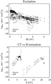 |
Fig. 5 Excitation (top panel) and ion-pair formation (bottom panel, CT stands for “charge transfer”) rate coefficients for Mn I and Mn II as used in this work and compared to Drawin’s formulae (Drawin 1968, 1969; Steenbock & Holweger 1984). |
3.2 Model atmospheres
As in our previous papers, we used MARCS (Gustafsson et al. 2008) and MAFAGS-OS (Grupp 2004a,b) model atmosphere grids. These are 1D LTE model atmospheres, with certain differences regarding the treatment of convective energy transport (mixing length), opacity, and the solar abundance mixture. The depth discretisation and the vertical extent of the models are also slightly different, as MAFAGS-OS covers the range from − 6 to + 2 in log τ5000, whereas the MARCS models sample the Rosseland optical depths from − 4 to + 2. Nonetheless, the thermodynamic structures of the models for the given input parameters are very similar (Bergemann et al. 2012, 2017).
The 3D model atmospheres are taken from the STAGGER model atmosphere grid (Collet et al. 2011; Magic et al. 2013)and computed with the STAGGER code (Nordlund & Galsgaard 1995). A 3D model consists of a series of computational boxes that represent a time series, which are referred to as snapshots. These snapshots are selected from a larger time series of snapshots that are produced from the STAGGER code and are selected at a time when they have reached dynamical and thermal relaxation. For our purpose and for the sake of time, we have chosen to work with five snapshots. Importantly, and unlike an equivalent 1D model, 3D models provide x, y, and z velocity fields for every voxel. This means that post-processing spectrum synthesis code provides parameter-free description of Doppler broadening, including asymmetric line profiles, which trace these gas flows at each voxel.
Figure 6 depicts the 3D temperature structures (blue 2D histogram) in a representative snapshot for four benchmark stars, along with the 1D MARCS (solid red line) and ⟨3D ⟩ (dashed grey line) profiles. The average temperature of the full 3D model and the 1D hydrostatic model are fairly different in the outermost regions of the atmosphere, as seen by comparing the 1D hydrostatic models with the ⟨3D ⟩ models. In particular, in the outer layers of metal-poor models the 1D hydrostatic models are significantly hotter (up to 500 K) compared to the 3D structures (see also Bergemann et al. 2017). Also the models diverge in deeper regions of the models, where the continuum usually forms. This is mostly due to the treatment of convection between the 1D and 3D model atmospheres.
The average temperature structure of the 1D model of the metal-poor RGB star HD 122563 is not very different from its ⟨3D ⟩ counterpart. Our adopted MARCS models are taken from Bergemann et al. (2012, their Fig. 1). We explore the impact of an adopted 1D model in Sect. 4.6, by performing the abundance analysis with a MAFAGS-OS suit of models. We also note that line formation is not only sensitive to the mean T(τ) and P(τ) structures, but also to the horizontal inhomogeneities. The latter play a significant role in the abundance analysis.
The scope of this paper is limited to the analysis of a small sample of 3D models, including that of the Sun, a typical dwarf, and a typical giant (Table 2). We also include tailored 3D models computed for the parameters of the benchmark metal-poor stars HD 122563, HD 140283, and HD 84937 (Sect. 2). To make the NLTE radiative transfer problem computationally tractable, we have to resample the full 3D model cubes onto a less fine, yet equidistant, grid in horizontal coordinates. However, we test the effect of the resolution of the cube for radiative transfer in Sect. 4.2 and find virtually no differences in the resulting atomic number densities and line profiles for horizontal resolutions of (x,y,z) = 30, 30, 230 and the original cubes ((x,y,z) = 240, 240, 230). Hence, the former is taken to be the default resolution for most of the analysis presented in this work. We solve the 3D NLTE radiative transfer problem for a set of snapshots for each of the 3D model atmospheres listed in Table 2. These snapshots are extracted at regular time intervals from the full simulation that covers roughly two convective turnover timescales (Collet et al. 2011; Magic et al. 2013). The convergence criterion, that is the maximum relative correction in the population numbers, max|δN∕N|, is set to 10−3. This is fully sufficient according to our experience with 1D NLTE radiative transfer.
3.3 Statistical equilibrium
We used two different codes to compute the SE of Mn. One is MULTI2.3 (Carlsson 1992), the other code is DETAIL (Butler & Giddings 1985). The codes solve the equations of radiative transfer and SE assuming a 1D geometry. The assumption of trace elements is used, that is, the element that is modelled in SE is assumed to have no effect on the model atmosphere. This is a good assumption for Mn as it is not an electron donor, nor does it have a high impact on the overall opacity. Both codes adopt the accelerated lambda iteration (ALI) technique and the operator acting on the source function.
The basic differences between the codes are described in Bergemann et al. (2012). The tests described in the following sections willbe performed imposing the same input conditions (LTE populations) and the same model atmospheres, in order to maximise the consistency. The main difference between the codes are in the handling of thermodynamic parameters and of the background opacities. In particular, DETAIL takes the partial pressures and partition functions from the input model atmosphere, whereas MULTI2.3 includes a package to compute these parameters given the input structures T(τ) and Pe (τ) as a function of optical depth or column mass.
In order to maximise the homogeneity of the analysis, we have also computed background opacity tables for MULTI2.3 using the updatedline lists from DETAIL (Bergemann et al. 2015). The MARCS (Gustafsson et al. 2008) and Turbospectrum (Plez 2012) codes were used to generate a table of opacities for a set of temperature and pressure points at more than 105 wavelengths, Mn6 lines being omitted. This table is then interpolated by MULTI2.3 to produce detailed line background opacities.
All calculations with MULTI2.3 are carried out by simultaneously solving the intensity at all angles, using the Feautrier method with all scattering terms included consistently (the ISCAT option set to 1). This is important when scattering in the background opacity is significant, as is the case in the Wien regime. We have tested the line formation disabling this option, but found that this has a very strong effect on the blue and UV lines of Mn I and Mn II, significantly over-estimating the line abundances,because of reduced continuum intensities.
MULTI3D is an MPI-parallelised, domain-decomposed NLTE radiative transfer code that solves the equations of radiative transfer in 3D geometry using the ALI method. The formal solution of radiative transfer is done via the short characteristics method (Kunasz & Auer 1988) that solves the integral form of the radiative transfer equation across one subdomain per time step. Carlson (1963)’s A4 quadrature is employed to compute the angle-averaged radiation field in the SE solution. The approximate operator is constructed using the formulation developed by Rybicki & Hummer (1991, 1992), where only the diagonal of the full Λ operator is used (for discussion of this approximation, see, e.g. Bjørgen & Leenaarts 2017).
MULTI3D will accept three types of 3D model atmosphere formats, including the commonly used Bifrost (Gudiksen et al. 2011) and STAGGER models (Magic et al. 2013). The code will also accept any 3D model providing the temperature, density, electron number density, and x, y, and z velocity fields are supplied on a Cartesian grid that is both horizontally periodic and equidistantly spaced. The code can compute radiative transfer using the 1.5D approximation, which treats each column of grid points in a model as a separate plane-parallel atmosphere, or using full 3D radiative transfer. The rate equations are assumed to be time-independent and the advection term is not included. For more information about the code, we refer to Leenaarts et al. (2012) and Bjørgen & Leenaarts (2017).
 |
Fig. 6 3D, 1D, and ⟨3D⟩ temperature structures as a function of Rosseland optical depth for benchmark stars. The blue-shaded regions indicate the kinetic temperature distributions in the representative snapshot from the 3D convection simulations. The stellar parameters are given in the inset. We note that ⟨3D ⟩ models are provided only to illustrate the difference between the average structure of the 1D and 3D models, however, the ⟨3D ⟩ are not used in our abundance analysis. |
Parameters of 3D convective and 1D hydrostatic model atmospheres.
4 Results
We begin the discussion of results with a brief account of NLTE effects in Mn (Sect. 4.1). The key properties of the statistical equilibrium of Mn are summarised in Sect. 4.1.1. 1D NLTE abundance corrections across a large parameter space are presented in Sect. 4.1.2. Line formation and abundances determined using 3D inhomogeneous atmospheres are the subjects of subsequent sections. Section 4.2.1 deals with the properties of line formation in full 3D solar simulation cubes, that we refer to as photon kinematics. In Sect. 4.2.2, we discuss simplified radiative transfer models and explore how these impact the line profiles compared to the full 3D NLTE solution. The results of the 3D NLTE solar abundance analysis are presented in Sect. 4.3. In Sect. 4.4, we discuss the impact of 3D NLTE on the line profiles, on their equivalent widths (EW), and on the abundance diagnostic for four metal-poor models. The results of LTE and NLTE calculations with 3D models are discussed in Sect. 4.5. Finally, in Sect. 4.6, we use 3D convective models of the benchmark metal-poor stars HD 84937, HD 140383, and HD 122563 to derive 3D NLTE abundances.
4.1 1D NLTE
4.1.1 Departures from LTE
This work does not deal extensively with the properties of statistical equilibrium of Mn nor with the details of line formation, as this has been discussed in great detail in our previous work (Bergemann & Gehren 2007). Additionally Bergemann & Gehren (2008) address the details of line transfer in metal-poor stars. It suffices to remind the reader that Mn, similar to other Fe-group elements, is a photo-ionisation dominated ion. Simply stated, the large photo-ioinisation cross-sections of Mn I energy levels imply significant over-ionisation in the atmospheres of cool stars in the more general SE case compared to LTE. Mn I becomes significantly over-ionised (compared to LTE) in metal-poor or in hotter stellar atmospheres due to their strong UV radiation fields. The effect of the radiation field is furthermore amplified in the atmospheres of giants owing to their lower densities and hence, less efficient collisional processes.
The effect of the radiation field is reflected in the behaviour of Mn I level departure coefficients, bi, which describe the ratio between NLTE and LTE atomic number densities. Departures from LTE take place in the line formation layers. Figure 7 shows that for Mn I, this ratio is typically ≲ 1, as in NLTE the fraction of atoms in a given energy state is less than that predicted by the Saha–Boltzmann formulae. The departure coefficients of the ionic levels, Mn II, are very close to unity for the lower-lying energy levels, but deviate from thermal for the levels of higher excitation energy, E ≳ 1 eV.
Figure 7 shows that the departures from NLTE in the line-formation region, − 2 ≲ log τ5000 ≲ 0, are moderate in the solar atmosphere, but only slightly smaller than our previous estimates in Bergemann & Gehren (2007). The differences with respect to the latter study are caused by the use of new quantum-mechanical photo-ionisation rates and H collision rates, as well as the implementation of fine structure for most of the Mn I levels. Collisions with electrons are not important in the physical conditions of the solar atmosphere. On the other hand, inelastic collisions with H atoms have a non-negligible effect on the atomic level populations and significantly contribute to the overall thermalisation of the system. This effect is not linear and may increase or decrease the departures from LTE for individual energy levels, and hence spectral lines, depending on the Teff, log g, and metallicity of a star.
The comparison of the bi profiles computed using DETAIL and MULTI2.3 (Fig. 7) suggests that the codes are consistent, given the same input conditions, such as the model atom, line opacities, and model atmospheres. MULTI2.3 predicts slightly larger departures from LTE compared to DETAIL. This has also been shown in our earlier paper for Fe (Bergemann et al. 2012), and is likely related to continuum opacities and/or the numerical implementation of the coupled SE and radiative transfer equations.
The behaviour of departure coefficients is very different in the model atmosphere of a metal-poor red giant star (Fig. 8). All Mn I levels show a stronger under-population compared to the solar model, implying larger differences between LTE and NLTE abundances in metal-poor stars. The energy levels of the Mn II lines are also affected by NLTE. In particular, the levels of the upper term  experience overpopulation caused by the radiative pumping in nine strong near-UV lines of Mn II multiplet Nr. 31 (a 5D–z 5Po) in the deeper layers. However, the levels of z 5Po become under-populated at log τ5000 ~ −1.5, as these lines progressively become optically thin. Consequently, one would expect significant NLTE effects on the formation of Mn II lines, largely driven by the changes in the line source function itself. Comparing the departure coefficients computed using the old atom from Bergemann & Gehren (2008) (Fig. 8, top panel) and the new atom in this work (Fig. 8, middle panel), we find substantial differences. The influence of new quantum-mechanical collisions with hydrogen is admittedly greater in the new atom, despite the larger photo-ionisation cross-sections. On the other hand, contrasting the results obtained using the DETAIL code with MULTI2.3 (Fig. 8, middle and bottom panels) confirms that, similar to the Sun (see Fig. 7), the two codes produce quantitatively similar outputs. In the outer layers, the departures are slightly different, which could be related to the differences in the outer boundary conditions.
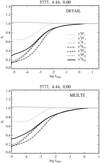 |
Fig. 7 Mn departure coefficients for solar MARCS model atmosphere as a function of optical depth at 5000 Å, computed using DETAIL (top panel) and MULTI (bottom panel) codes. The surface parameters of the Sun, (Teff, log g, and [Fe ∕H]) are given in the figure details. |
4.1.2 NLTE abundance corrections
An NLTE abundance correction is the quantity that is commonly used in stellar abundance studies to correct the abundances derived under the assumption of LTE. The abundance correction is defined as Δ = A(NLTE) − A(LTE), that is the difference in abundance required to fit a given spectral line assuming 1D LTE or 1D NLTE. We also employ this concept in our 3D NLTE analysis in Sect. 4.2.
Figure 9 illustrates the NLTE abundance correction for several metal-poor models in the metallicity range − 3 to 0. We only plot selected lines to illustrate the key results: the 3488 Å line of Mn II, multiplet 4 (4030, 4033, 4034 Å), multiplet 18 (4783, 4823 Å), and multiplet 32 (6013, 6016, 6021 Å) of Mn I. The behaviour of abundance corrections within a given multiplet is very similar, hence the lines aregrouped by multiplets. The correction is not tailored to any particular star and is computed assuming the reference NLTE [Mn∕Fe] of zero. We also explored the abundance corrections computed using LTE [Mn∕Fe] abundance of − 0.5 to − 0.8, as it would be typically measured assuming LTE in metal-poor stars and found no significant differences in the corrections. The individual curves represent three possible scenarios that differ in the completeness of the model atom.
In Fig. 9, we illustrate the sensitivity of the corrections to the quantum-mechanical H data. The CH case (note that CH is not an abbreviation) corresponds to the model atom, which is devoid of quantum-mechanical H-collisionalexcitation processes (but includes charge transfer). The CH0 model lacks charge transfer processes, but includes collisional excitation. These two cases are compared to the model, which has both excitation and charge transfer (CH/CH0 included). None of the three cases presented in this figure includes the Kaulakys (1985) collision rates.
The H collisions clearly have a different impact on the line formation in the atmospheres of giants and dwarfs. Based on the NLTE abundance corrections in the figures, it appears that for dwarfs, H collisions serve as a thermalising agent, decreasing the difference between NLTE and LTE. In the atmospheres of red giants, the effect is somewhat counter-intuitive: the lines of multiplet 32 (6013–6021 Å triplet) have smaller NLTE corrections when H collisions are excluded. In fact, this is the indirect effect of over-ionisation, which is more efficiently transferred to higher-excitation states by collisions with H. On the other hand, the lines of multiplet 18 (4783, 4823 Å) behave as expected from the simple considerations of increased rate of collisional thermalisation. Figure 9 also suggests that charge transfer (CT) reactions are more important in the atmospheres of dwarfs. Neglecting CT fully typically leads to abundance corrections being over-estimated by 0.05 dex for the models with [Fe∕H] ≿ −3.
Figure 10 illustrates the influence of collision rates computed using the Kaulakys (1985) recipe. The reference atom includes the Kaulakys (1985) collisions in addition to the data from Belyaev et al. (2017), and we compare this model with the model that is devoid of the Kaulakys data. The differences with our reference model atom are modest, and do not exceed 0.05 dex for the dominant part of the parameter space. The effects that are possibly most significant occur when we neglect Kaulakys (1985) collisions. This leads to slightly over-estimated NLTE abundance corrections for the multiplet 32 Mn I lines (6013 – 6021 Å triplet) in the RGB models. On the other hand, the NLTE abundance corrections for these very high-excitation lines are systematically under-estimated in the model of a dwarf.
The general picture is that the NLTE abundance corrections for the Mn I lines are positive and increase with decreasing metallicity, supporting our earlier study of Mn (Bergemann & Gehren 2007, 2008) and of other similar ions (e.g. Fe, Bergemann et al. 2012; Lind et al. 2012). The corrections are slightly larger for the RGB model, especially at lower [Fe∕H]. The higher-excitation lines, such as those of multiplets 18 and 32 are more sensitive to NLTE. Their NLTE abundance corrections typically increase with decreasing metallicity, but this trend slightly flattens below [Fe/H] ~ −2. Another noteworthy feature of these diagrams is the fact that the Mn II lines are also not immune to NLTE. It has been often assumed in the literature that the lines of ionic species do not show NLTE effects. The few strong excited lines of Mn II at 1.85 eV show the classical NLTE effect of photon loss. This effect is small, but shows in the atmospheres of dwarfs and giants (see Fig. 10). It implies that lower abundances would be obtained from Mn II line, especially for the metal-poor stars with [Fe∕H] = −2. At lower metallicity, the Mn II lines become sufficiently weak and radiative pumping effects dominate, leading to positive NLTE abundance corrections.
It is interesting, and it possibly presents the main difference with respect to our earlier study, that the strong resonance triplet of Mn I at 4030–4034 Å and the excited lines show very similar NLTE abundance corrections. The NLTE corrections exceed just about 0.4 dex in the atmospheres of RGB stars with [Fe/H] = −3. This is important, as LTE abundances derived from the resonance Mn I lines are known to be significantly lower compared to high-excitation Mn I features (Bonifacio et al. 2009; Sneden et al. 2016). Compared to the high-excitation features, in the 1D NLTE analysis there is no room for differentially larger NLTE corrections for the 4030–4034 Å triplet lines. In our previous work, a higher degree of over-ionisation in Mn I, and, in particular, over-ionisation from the ground state, was achieved by employing a tailored SH scaling factor to the Drawin collisional (excitation and ionisation) Mn I + H I rates. As a consequence, the NLTE abundance corrections for the resonance triplet lines were significantly higher.
Below we show that 3D NLTE calculations suggest substantial differential effects between Mn I lines of different excitation potentials. These differential effects help to improve the excitation balance (Sect. 4.2), effectively providing the physical basis for the effect, which is mimicked by using inefficient H collisions in 1D models.
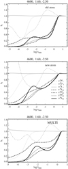 |
Fig. 8 Mn departure coefficients for model atmosphere of a metal-poor red giant. These were computed using the old Mn atom from Bergemann & Gehren (2007) (top) and the new atom from this paper (middle panel: DETAIL, bottom panel: MULTI). The stellar parameters (Teff, log g, and [Fe ∕H]) are given in the figure titles. |
 |
Fig. 9 NLTE abundance corrections for Mn I (4030, 4033, 4034, 4783, 4823, 6013, 6016, and 6021 Å) and Mn II (3488 Å) lines. These are computed for a small grid of MARCS model atmospheres representative of dwarfs: Teff = 6000, log g = 4.0 (top panels),and red giants: Teff = 4500, log g = 1.5 (bottom panels) for a range of metallicities from 0 to − 3 dex. Different curves represent the corrections derived using the model atoms with reduced complexity: (a) CH excluded, ignoring the excitation processes by collisions with H atoms; (b) CH0 excluded, ignoring the charge transfer reactions; and (c) CH∕CH0 included with excitation and CT rates from the quantum-mechanical calculations. None of the three models (a–c) include the Kaulakys recipe. |
 |
Fig. 10 NLTE abundance corrections for Mn I and Mn II lines. These are computed for a small grid of MARCS model atmospheres representative of dwarfs: Teff = 6000, log g = 4.0 (top panels),and red giants: Teff = 4500, log g = 1.5 (bottom panels) for a range of metallicities from 0 to − 3 dex. Different curves represent the corrections derived using two model atoms, one with and the other without collisions derived using the Kaulakys recipe. |
4.2 3D NLTE
4.2.1 Photon kinematics
Figure 11 illustrates spatially-resolved NLTE intensity profiles of two Mn I lines in the solar model at the disc centre. All profiles are normalised to the average continuum intensity for the corresponding spectral line in the snapshot. The lines were chosen such that the effect of the HFS is minimal, in order to isolate the effect of granular motions on the profiles. The profiles are taken for every fourth point along each horizontal coordinate in the simulation domain (i.e. for 8 × 8 = 64 points out of 900) in order to not overload the figure. The bisectors for each line component are shown in the right-hand side panels. In addition, the solid curves indicate the profiles extracted from the granule and inter-granular lane in Fig. 12.
Overall, the behaviour of the lines is very similar to that described earlier by Dravins & Nordlund (1990a, for example in their Fig. 6 for a Sun-like star α Cen A). The weaker high-excitation Mn I line at 5004 Å shows a strong anti-correlation between the depth of the line core and the line shift (right-hand panel). This is, in fact, the weakest unblended solar Mn I line with the EW of only 13 mÅ. The line profiles with the strongest blue-shift and the highest intensity contrast form above the granules, where the upwards streaming motions of hotter material are characterised by higher velocities, and higher granular temperatures account for the brighter background continuum. The dominant NLTE effect of over-ionisation leads to brightening in the line core. The lack of any pronounced curvature in the bisectors of the blue-shifted components suggests that there is little vertical variation of velocity field in the upflows.
The Mn I line at 4502 Å, which is stronger but has the same lower excitation potential as the 5004 Å line, also shows a very broad distribution of line shifts. This line is close to saturation, as is evidenced by the broad, rectangular inner core in the bluest components. Similar to the 5004 line, the bisectors of the blue-shifted components, which form above granules, are typically l-shaped, that is, the line profiles are nearly symmetric. Although the blue-shifted components are very strong, and are characterised by very (vertically) extended line-formation regions, this again suggests that the vertical variation of velocity fields in the granules is small. On the other hand, the bisectors of the profiles that form above the inter-granular lanes tend to approximate a c-shape. These line components are highly asymmetric, their cores are very broad, and tend be skewed to the red. Dravins & Nordlund (1990a) found that this is a characteristic feature of the lines that form across inter-granular regions with a larger vertical-velocity gradient with depth.
4.2.2 3D test cases
Calculations of 3D NLTE radiative transfer are very computationally expensive. Hence, we explored whether a simplified treatment of NLTE radiative transfer with 3D simulations offers a suitable alternative to full 3D NLTE calculations.
In particular, we illustrate and discuss the results of calculations obtained using more compact model atmosphere cubes and different radiative transfer solvers (1.5D versus full 3D). We also compare the flux profiles obtained using different solar snapshots. In what follows, we limit the discussion to two Mn I lines only. One of them is a strong resonance line at 5394 Å, where the effects of NLTE and 3D convection are most pronounced. The second line is that at 4502 Å, discussed in the previous section. This line is least affected by the HFS, hence its shape is a good test case to explore the effects of NLTE and 3D convective flows.
The top left panel of Fig. 13 shows the line profiles computed in full 3D NLTE versus 1.5D calculations (Sect. 3.3). The difference is negligible and it amounts to less than 0.5% in the flux level, or <0.01 dex in abundance, that is, far less than the uncertainty incurred by the other sources of error. In the case of metal-poor stars, the differences are also modest and do not exceed a few percent in EW. Since the computational time of 3D NLTE scales as O(n4∕3), where n is the number of grid points (meaning the number of iterations is proportional to the number of grid points in the z direction), it is a reasonable approximation to use 1.5D NLTE calculations, at least for the stars with parameters similar to the models tested in this work.
The top right panel of Fig. 13 illustrates the impact of the model atmosphere resolution. We employ three models: one resampled to the resolution of 5 × 5 × 102, the other with the resolution of 30 × 30 × 230 (our default resolution), as well as the maximum resolution of 100 × 100 × 230 that we can afford with the computing time available to us. The comparison of the medium- and maximum- resolution simulation can be found in the appendix. The effects are visible in the line profiles, but they only slightly change the shape of the line and have a very modest effect on the line equivalent width. This effect comes mostly through the impact of velocities on the line opacity, κ(x, ν × (1 − ν(x)∕c)) as is best seen in lines that are not very sensitive to HFS, such as the 4502 Å line (left panel in Fig. 13). Their shapes are closely approximated by a Gaussian fit, and the effects of velocity fields are easily distinguished. In particular, the red wing of the line appears to be slightly darker in the model with higher resolution. There is also an implicit effect of velocities on the line source function, as it depends on the radiation field at the line frequencies, which is non-local and connected to the velocity distribution at all spatial points along the beam.
We also find (Fig. 13, bottom left panel) that the flux profiles computed using different (regularly-spaced in time) snapshots do not show significant variations. The 5394 Å line changes its depth by ~ 3%. The position of the line centre changes by a few mÅ. The 4502 Å line is almost insensitive to the temporal effects. This suggests that the statistical properties of velocity fields, temperature, and pressure inhomogeneities in each snapshot are representative of some average distribution values for the relaxed simulation given the values of Teff, log g, and [Fe ∕H]. The temporal variability of spatially resolved profiles has been examined in detail in Dravins (1990); Dravins & Nordlund (1990b, their Sect. 5). They found that the characteristic evolution of line shapes and depths lacks a unique timescale, that was a manifestation of the lack of a unique scale in the spatial power spectra. Hence, the ensemble averages of spatially resolved line profiles are very similar in different snapshots, as we will also demonstrate in Sect. 4.4 for other models.
Finally, the bottom right panel of Fig. 13 illustrates the line profiles computed with 1D LTE and 3D NLTE. This is a major difference that amounts up to 0.2 dex in the abundance (see next section). Similar to the earlier studies for ions with similarly complex electronic structure, and ionisation potential (e.g. Amarsi et al. 2016; Lind et al. 2017, for Fe I), we find that the effects of 3D NLTE are to weaken the line compared to 1D LTE. Mn I is a photo-ionisation-dominated ion, that is the NLTE effects are driven by a strong non-local radiation field across multiple ionisation channels of the ion in the UV and in the optical. Of all Mn I lines, the resonance lines at 5394 and 5432 Å are most sensitive to this effect, as the lines are comparatively weak in the solar spectrum, and their NLTE effect is mainly caused by the change in the line opacity that scales in the first order as the ratio of the NLTE to LTE number densities of the lower energy level of the transition. The higher-excitation lines, such as that at 4502 Å show more modest NLTE effects in the model atmosphere of the Sun, both in 1D and in 3D.
The results of our test calculations indicate that vertical radiative transfer in NLTE with full 3D data cubes at the resolution of (x,y,z) = 30, 30, 230 is the most suitable approach and we employed this method in our calculations of Mn abundances for the Sun (Sect. 4.3) and the benchmark stars (Sect. 4.6). The approach allows affordable 3D NLTE calculations within reasonable timescales and provides line profiles consistent with the original resolution of the 3D cubes, as well as, with the full 3D radiative transfer calculations.
 |
Fig. 11 Spatially resolved line profiles (left panels) and their bisectors (right panels) for solar disc centre in model snapshot 020. The solid blue curve indicates the line profile extracted from the granule, whereas the red curves correspond to the inter-granular lane. The corresponding surface areas are marked with yellow and blue boxes in Fig. 12. |
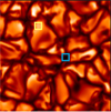 |
Fig. 12 Monochromatic image of solar granulation at wavelength of 5394 Å at solar disc centre. |
 |
Fig. 13 Comparison of theoretical profiles for Mn I lines at 4502 and 5394 Å for solar snapshot 020. Top left panel: 1.5D NLTE versus full 3D NLTE. Top right panel: line profiles computed with the 3D data cubes scaled down to the resolution of (x,y,z) = 30, 30, 230 (solid line) and 5, 5, 102 (dashed line). Bottom left panel: full 3D NLTE for the five solar snapshots. Bottom right panel: 3D NLTE profiles versus 1D LTE profiles. |
 |
Fig. 14 Comparison of 3D NLTE line profiles for selected Mn I lines with observed solar flux spectrum. All model profiles were generated using the same Mn abundance of 5.47 dex. |
4.3 SolarMn abundance
The Sun is a metal-rich star, and as such, the spectral lines in most cases appear to suffer from blending and/or strong sensitivity to damping or turbulence. As a matter of fact, most Mn I lines are not very useful, being either blended or too strong, with a few exceptions. Nonetheless, we start with the analysis of all Mn I lines that are typically used in the analysis of FGK stars, and later assume a more conservative approach that takes into account only the most reliable features.
The LTE analysis of the solar Mn I lines is carried out using the SIU spectrum synthesis code (Reetz 1999). SIU allows interactive spectral fitting, which is very convenient to test for the presence and effects of blends and asymmetries within a line. This is a very accurate approach, especially when applied to ultra-high-resolution spectra, such as the solar atlases, and has been commonly exploited in the literature.
Figure 14 presents some examples of 3D NLTE line profiles for the solar spectrum. Note that in this plot, we have not adjusted the Mn abundances, but assumed the abundance of 5.47 dex, as recommended by earlier studies of the solar Mn abundance. Most of the Mn I lines are very broad, with the width of 0.2−0.3 Å, which is a consequence of the HFS. It is obvious that the available atomic and HFS data describe the line profiles remarkably well, both in terms of the asymmetries and the multi-component structure. The latter is particularly prominent in the cores of the weak resonance or ground-state lines, such as the 5394 and 5516 Å line. The core of the line at 5420 Å is slightly too weak, compared with the observations. This could be due to its sensitivity to activity (Wise et al. 2018). Note that also the 5394, 5432, and 6013 lines could be affected (Wise et al. 2018), and in particular, the 5394 Å line has a long history of research owing to its variation with the global solar activity cycle (Danilovic & Vince 2005; Livingston et al. 2007). Some studies suggest that the line is not as sensitive to granular motions as other features, because of its wide HFS, and is more sensitive to the intergranular magnetic concentrations, similar to the CH G-band (Vitas et al. 2009). According to our 3D NLTE results, however, the 5394 Å line is sensitive to convection and shows a significant difference between modelling with 1D hydrostatic and 3D convective models. Overall, the agreement of the model 3D NLTE line profiles with the observed solar data suggests that the atomic data quality and the physical quality of spectral models are sufficient to satisfactorily describe the properties of Mn lines in the solar spectrum.
The abundances determined from the Mn I lines that we view as reliable photospheric abundance diagnostics are shown in Fig. 15. The major challenge in the analysis of the solar spectrum is the contamination of line profiles by blends. These are present in the wings of the strong Mn I lines, such as the 4761, 4762, 4765, and 4766 Å, but also the lines of multiplet 18 (4783 and 4823 Å). Besides, there are no quantum-mechanical data for elastic collisions with H atoms for the two latter lines (Barklem et al. 2000), hence, we have to resort to the standard Unsöld formalism that carries an additional source of an uncertainty. We disregard such lines when computing the solar abundance of Mn. The 1D NLTE and 3D NLTE Mn abundances are derived by applying the corrections computed using MULTI2.3 and MULTI3D for the individual spectral lines.
In 1D LTE, the low-excitation potential and/or very strong lines give a lower abundance of Mn compared to the high-EP (weaker) lines. The difference is not large, but significant given the very quality of the observed data and well-constrained fundamental parameters of the Sun. The effects on NLTE in the solar atmosphere are moderate and change the average solar abundance by only ~ 0.02–0.07 dex. NLTE alone does not help to improve the solar excitation balance. More important is the combined influence of convection and NLTE. In the case of NLTE calculations with the 3D convective solar model, the effect of over-ionisation is amplified owing to stronger background radiation fields in the granules. The 3D NLTE–1D LTE difference is equivalent to ~ 0.22 dex in abundance for the resonance lines, but 0.15 dex for the higher excitation lines of other multiplets.
Our solar abundances of Mn are 5.34 ± 0.04 dex in LTE, 5.41 ± 0.05 dex in NLTE, and 5.52 ± 0.04 in 3D NLTE. The 1D NLTE and 3D NLTE values are consistent with the meteoritic abundance of Mn 5.50 ± 0.03 dex reported by Lodders (2003). Our 1D LTE result is ~0.1 dex higher compared to the previous estimate reported in Bergemann & Gehren (2007), 5.23 ± 0.1 dex. On the other hand, it matches very well with our LTE estimate obtained using the MAFAGS solar model, the revised transition probabilities, and the SIU spectrum synthesis code in Blackwell-Whitehead & Bergemann (2007), 5.33 ± 0.1 dex. The new 1D NLTE values are also higher than the estimates in Bergemann & Gehren (2007). In both cases, 1D LTE and 1D NLTE, the difference is due to the revision of the transition probabilities and the NLTE model atom.
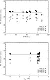 |
Fig. 15 Mn abundances determined from individual Mn I lines in solar flux spectrum using different models: 1D LTE, 1D NLTE, and 3D NLTE. The solid line denotes the Mn abundances measured in CI chondrites, 5.50 ± 0.03 dex (Lodders 2003). |
4.4 3D NLTE effects in metal-poor model atmospheres
Our analysis of line formation with 1D models suggests that the majority of Mn lines are sensitive to NLTE. Also the calculations for the 3D hydrodynamical model of the Sun indicate a strong impact of convection on the line profiles,which does not cancel the NLTE effects, but rather amplifies them for the most spectral features of Mn I.
In this section, we present the analysis of line formation in several model atmospheres of metal-poor stars. We explore the models with parameters with Teff = 6500 K, log g = 4 dex, [Fe ∕H] = −1 and Teff = 4500 K, log g = 2, [Fe ∕H] = −1, as well as their metal-poor counterparts with [Fe∕H] = −2. For simplicity and didactic clarity, all calculations were performed assuming a scaled solar Mn abundance. Deviations from this assumption may affect the line formation, yet at this stage we are interested in the combined effects of 3D radiative transfer in convective models and NLTE and the impact on Mn I lines with different properties. We explore which lines are least sensitive to these effects, and employ them in the abundance analysis in the follow-up study of a larger stellar sample.
Our results for the four 3D models are illustrated in Fig. 16. We also overplot the predictions of 1D LTE modelling computed using the same Mn model atom and the same Mn abundance. Similar to the solar model, the 3D NLTE line profiles are much weaker than the 1D LTE counterparts. This is the consequence of over-ionisation, which is stronger in metal-poor conditions due to reduced line blanketing and stronger UV radiation fluxes. The topology of convection in FGK stars is set by mass conservation. The hotter rising granules occupy the dominant (~ 2∕3) part of the stellar surface, whereas the cooler downdrafts are confined to narrow inter-granular lanes (Stein & Nordlund 1989; Nordlund et al. 2009), although the area subtended by the down-flows increases with depth. Hence, over-ionisation in the granules is the dominant NLTE effect that defines the appearance of the spatially integrated line profiles. In contrast to the Sun, where the effects of convective shifts were marginal, the integrated flux profiles in the metal-poor models show strong asymmetries, with typical blue-shifted cores and skewed wings. This is best seen by comparing the symmetric 1D profiles, convolved with an arbitrary macro-turbulence and the 3D profiles, which do not assume any ad-hoc broadening. Also the line profiles from individual snapshots are remarkably similar to their temporarily averaged counterparts, although a slightly more pronounced temporal variation is seen in the NLTE line profiles computed using the 3D models of dwarfs (as in Fig. 16).
The differences between 1D LTE and 3D NLTE profiles are very large, with only a few notable exceptions. These exceptions are the blue lines of Mn II, such as the 3488 and 3497 Å lines. For dwarfs, these low-excitation Mn II features are nearly invariant to the changes in the model atmosphere structure, and they indeed show very similar line shapes and equivalent widths, regardless of whether one adopts LTE or NLTE radiative transfer. Also a standard choice of the micro-turbulence ξt = 1 km s−1 appears to be satisfactory for a dwarf model, producing a line profile, which closely resembles the full 3D NLTE profile of the Mn II 3488 Å line even in the model with [Fe∕H] = −2. For the computational complexity of 3D NLTE modelling, we are unable to explore a larger parameter space of 3D models in this work, but the behaviour of the models with metallicity suggests that this conclusion may hold also for other stars on the main-sequence, as long as [Fe ∕H] is not in the extremely metal-poor domain.
This fortunate result does not hold for the atmospheres of giants, however, and neither does it generally hold for the Mn I lines. The 3488 Å line of Mn II suffers from non-negligible deviations from NLTE in the RGB models, being significantly stronger in 3D NLTE. On the other hand, the 3D NLTE abundances of all lines of Mn I are significantly higher compared to 1D LTE. This is best illustrated by exploring the differences between 1D LTE and 3D NLTE, and 1D NLTE and 3D NLTE abundances derived from the line of a given equivalent width. This quantity is typically referred to as a 3D NLTE abundance correction (3D NLTE – 1D LTE).
The top panel of Fig. 17 shows that the 3D NLTE abundance corrections amount to 0.25 dex for most Mn I lines in the atmospheres of dwarfs, but in the models of RGB stars the (3D NLTE – 1D LTE) abundance differences tend to be significantly larger. In all cases, 1D analysis tends to substantially underestimate the Mn abundance. In particular, for the lines of multiples 18 and 32 (e.g. 4823 and 6016 Å) we find the abundance corrections of 0.3–0.4 dex in metal-poor models, whereas the blue resonance lines at 4030–4034 Å show even larger 3D NLTE corrections of ~ 0.5 dex at [Fe ∕H] = −2. This is a very interesting result. On the one hand, our results suggest that the large abundance discrepancies and excitation imbalance seen in the analysis of RGB stars (Bonifacio et al. 2009) may indeed be accounted for by 3D NLTE. On the other hand, we also find that 3D NLTE effects do not significantly impact the excitation balance in the atmospheres of very metal-poor dwarfs, as 3D NLTE corrections are similar for the lines of all Mn I multiplets. This is why this effect may go undetected in 1D LTE studies of stars with similar parameters (e.g. the study of HD 84937 by Sneden et al. 2016, or Mishenina et al. 2015). Also the 3D NLTE corrections for the Mn II lines are very small in the metal-poor atmospheres of dwarfs, and do not exceed − 0.05 dex at [Fe/H] = −2.
Figure 17 also suggests that, whereas 1D LTE always underestimates abundances for the Mn I lines, there are a few Mn I lines that can be reliably modelled with 1D NLTE. These are the lines of multiplets 9 (e.g. 4055, 4070, and 4082 Å), 23 (e.g. 4761, 4762, 4765, and 4766 Å), 24 (e.g. 4436, 4451, 4498, and 4502 Å), and 32 (e.g. 6013, 6016, and 6021 Å). For these features, the differences between 1D NLTE and 3D NLTE are marginal, and do not exceed 0.1 dex in the lowest metallicity ([Fe/H] = − 2) models of both dwarf and RGB stars. The lines of other multiplets show a very significant systematic deviation from 1D NLTE, caused by the impact of convective inhomogeneities. Additionally, for dwarfs, the impact of convection is modest and indeed, most optical Mn I lines, including the resonance Mn I triplet at 403 nm, would be suitable for abundance diagnostic, leading to a modest bias of  dex. The exact value would also depend on the abundance of Mn itself, and additionally on the assumed value of micro-turbulence in the 1D models. So our estimates of 3D NLTE abundance corrections may not be directly applicable to the 1D LTE measurements in the observed stars. Rather we recommend employing those lines, which according to our tests, show minimal impact of convection and/or NLTE.
The IR lines of Mn I, like those that are used in the H-band abundance analysis (Shetrone et al. 2015), show significant departures from 1D and LTE. However, it is remarkable that all three Mn lines that we tested in this work show very similar 3D NLTE – 1D NLTE differences in dwarf and RGB models. In effect, the abundances for all these models are systematically underestimated by − 0.15 dex with respect to 1D NLTE, and the bias appears to be insensitive to metallicity of the model. It appears reasonable then to apply a positive correction to all H-band Mn 1D NLTE abundance measurements to obtain physically unbiased results.
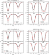 |
Fig. 16 Line profiles of selected Mn I lines in dwarf and RGB models with metallicities [Fe ∕H ] = −1 (top panels) and [Fe∕H] = − 2 (bottom panels). Thick solid curves correspond to the averaged profiles from five snapshots taken at equidistant time steps. Thin lines are the profiles from individual snapshots. 1D LTE profiles are computed assuming ξt = 1 km s−1. The 1D LTEprofiles would be stronger, if larger ξt values were assumed. Note that different spectral lines of Mn I and Mn II are shown in the panels. |
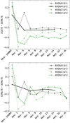 |
Fig. 17 3D NLTE abundance corrections for selected models. |
4.5 3D LTE versus 3D NLTE
Figure 18 compares the line profiles computed using 3D LTE, 3D NLTE, and 1D LTE. The latter is convolved with a macro-turbulence of 4 km s−1.
For the [Fe/H] = −1 dwarf model, the 3D LTE line profile of the Mn II line at 3488 Å closely resembles the equivalent 1D LTE profile. The Mn I lines at 4766 and 6021 Å are slightly shallower in 3D LTE compared to 1D LTE, but deeper for the 4823 Å line. On the other hand, all lines of Mn I are much fainter in 3D NLTE compared to 3D LTE, suggesting that a 3D LTE analysis would strongly underestimate the Mn abundances.
This tendency is qualitatively very similar in the dwarf model at [Fe/H] = −2. One notableexception is that the resonance line at 4034 Å is now exceptionally strong in 3D LTE, much stronger than the profiles computed using 1D LTE and 3D NLTE. This behaviour is also known for strong resonance lines of other chemical species. The major implication of this is that 3D LTE modelling is unlikely to solve the excitation imbalance in Mn, which is well-known from 1D LTE studies (e.g. Bonifacio et al. 2009; Sneden et al. 2016). The unfortunate problem is that even in 1D LTE the resonance Mn I lines yield significantly lower abundances, relative to their higher excitation counterparts. The 3D LTE line profiles of the resonance lines are stronger than their 1D LTE counterparts, computed assuming the same Mn abundance, meaning that the 3D LTE abundances of these lines must be reduced to recover the correct equivalent width. For the higher-excitation lines, the differences between 1D and 3D LTE at [Fe/H] = −2 are not large, because the lines are very weak, and form deep in the atmosphere, at log τ5000 > −2, where the temperature inhomogeneities are not pronounced and the average structure of the 1D hydrostatic models closely resembles that of 3D models (see, e.g. Fig. 6).
The behaviour is very similar in the 3D models of giants. 3D LTE line profiles are not too different from 1D LTE at [Fe/H] = −1 despite the modest effect of convection on the line shapes, but they are always stronger compared to 3D NLTE. The differences are exacerbated at low metallicity, [Fe/H] = −2, where 3D LTE calculations greatly overestimate the strength of all Mn I lines compared to 3D NLTE. The UV Mn II line at 3488 Å shows very small NLTE effects in the metal-poor RGB model, in fact, its 3D LTE and 3D NLTE profiles are very similar. On the other hand, the 1D LTE assumption underestimates the strength of the Mn II line, thus overestimating the Mn abundance derived from this feature.
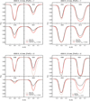 |
Fig. 18 Same as Fig. 16, but thick dotted-dashed brown curves now denote the profiles from 3D LTE calculations for the same five snapshots. |
4.6 Benchmark metal-poor stars
The Mn abundances in the stellar spectra were computed by matching the observed equivalent widths to the grids of 1D LTE and 1D NLTE spectral lines computed using MULTI2.3. The equivalent widths were measured from the UVES-POP spectra of these stars using the SIU code. Unlike in our analysis of the Sun, we have chosen to not employ SIU for abundance measurements in metal-poor stars, as blending is not a problem anymore and a detailed spectrum synthesis is unnecessary. Also MULTI2.3 has an advantage in that it includes background scattering, which is essential for the blue and UV lines. 3D NLTE corrections were computed separately and applied to the 1D LTE abundances derived using the measured EWs.
The results for all three benchmark metal-poor stars are shown in Fig. 19. The error bars correspond to the uncertainties of the EW measurements. We show the abundances derived using the MAFAGS-OS models (left panels) and the MARCS models (right panels) in order to illustrate the impact of the 1D model atmospheres. Overall, the results obtained MAFAGS-OS and MARCS models are in agreement, especially for the model of the metal-poor RGB star HD 122563. The differences can generally be explained by the small differences in the input parameters of the models. In particular, the MAFAGS-OS models assume the following parameters: (a) HD 122563: Teff = 4600 K, log g = 1.60 dex, [Fe/H] = − 2.5 dex; (b) HD 140283: Teff = 5773 K, log g = 3.66 dex, [Fe/H] = − 2.38 dex; and (c) HD 84937: Teff = 6350 K, log g = 4.09 dex, [Fe/H] = −2.15 dex. This is most likely at the origin of the somewhat lower abundances that we get for HD 84937. It is also noteworthy that MARCS models lead to slightly more consistent abundances from Mn I lines for all three reference stars.
Regardless of the choice of 1D models, 1D LTE modelling reveals a significant ionisation imbalance, in that the Mn I lines give systematically lower abundances compared to Mn II lines, confirming the results reported in the literature (Johnson 2002). The difference is most pronounced for the RGB star HD 122563, for which the offset is close to 0.7 dex. We also confirm the Mn I excitation imbalance in all three stars, with strong resonance lines of Mn I producing systematically lower abundances compared to higher excitation lines. For HD 122563, the offset between the lines of multiplet 4 (the 4030–4034 Å triplet) and the lines of other multiplets is ~ 0.2 dex, whereas for the subgiant HD 140283 and turn-off star HD 84937 the offset is slightly larger, of the order ~ 0.3 dex.
The ionisation balance is significantly improved for all three stars in 1D NLTE. In particular, for HD 84937 and HD 140283, the abundances derived from the high-excitation lines are now consistent with the abundances derived from the Mn II lines. For HD 122563, the ionisation balance in 1D NLTE is only partially improved, but there is still a differential effect of − 0.2 dex for the high-excitation lines and − 0.5 dex for the low-excitation lines.
The improvement is most striking in 3D NLTE. The 3D NLTE abundance corrections are very large and positive for both ionisation stages. For HD 122563, this brings Mn I and Mn II lines into agreement. For HD 84937 and HD 140283, the 3D NLTE abundances are higher compared to 1D NLTE, however, the differential effect is not as large. It should be emphasised that stellar parameters of these three stars are well-constrained by independent methods, and the fact that ionisation balance is satisfied in 3D NLTE, without resorting to ad-hoc parameters, like micro-turbulence in 1D, is remarkable. For comparison, to explain the ionisation imbalance in HD 122563 by the error in stellar parameters, its Teff would have to be increased to 4900 K (that would bring the resonance lines up by approximately +0.7 dex to be consistent with Mn II), or alternatively the ξt increased to 3.5 km s−1 dex that would push the Mn II abundances down by approximately − 0.7 dex. Decreasing the log g might help to increase the abundance from the resonance lines, but a change to log g < 0.5 would be necessary. All these changes in stellar parameters can be ruled out, given the robust constraints from asteroseismology and interferometry (Creevey et al. 2012; Karovicova et al. 2018; Creevey et al. 2019). Also micro-turbulence, despite being a free parameter, is relatively well-constrained in the literature (Bergemann et al. 2012; Afşar et al. 2016).
Sneden et al. (2016) recently analysed HD 84937 by employing 1D LTE models. They adopted somewhat different stellar parameters for this metal-poor turn-off star: Teff = 6300 K, log g = 4.0, [Fe ∕H] = −2.15, and ξt = 1.5 km s−1. Their estimates of [Mn/Fe] for this star are approximately − 0.25 for the Mn II lines and approximately −0.3 for the Mn I lines (their Fig. 7). On the other hand, they also tabulate the abundances derived by taking the ratios of the elements derived from the lines in the same ionisation stage (e.g. Mn I to Fe I and Mn II to Fe II). In the latter case, their values are −0.42 for the Mn II lines and −0.46 for the Mn I lines (their Table 5).
Our 1D LTE estimates for HD 84937 are [Mn/Fe] = − 0.24 dex, as derived from the Mn II lines, and [Mn/Fe] = −0.47 dex for the high-excitation Mn I lines. Similar to Sneden et al. (2016), we find that the Mn I triplet lines give the abundances that are ~ 0.2 dex lower compared to the high-excitation lines. Our abundances derived from the Mn I lines may appear to be lower, but this is likely the consequence of the adopted metallicity. Indeed, we adopt [Fe ∕H] = −2.0 dex in this work. This is consistent with our ⟨3D⟩ NLTE estimate in Bergemann et al. (2012), where we found metallicities in the range from [Fe ∕H] = −2.04 to −1.95 dex, depending on the choice of the H-scaling factor. Amarsi et al. (2016) find [Fe/H] = −1.96 ± 0.02(stat) ± 0.04(sys) dex from the full 3D NLTE Fe analysis. On the other hand, Sneden et al. (2016) adopt a very low metallicity, [Fe ∕H] = −2.15 dex, that leads to significantly higher Mn abundances. It is not clear which of the estimates from Sneden et al. (2016) are to be given preference and which of their two methodological approaches is more consistent with our estimate. Contrary to that study, we do not consider lines with EWs ≲ 3 mÅ in the UVES spectrum of HD 84937 as reliable, such as the lines at 4762, 4765, 4766 Å, and the red triplet at 6013–6021 Å. This, combined with the choice of the atmospheric models, stellar parameters, and methods to determine the abundances, may account for the somewhat different results in our study and in Sneden et al. (2016).
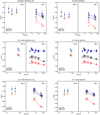 |
Fig. 19 Mn abundances in three metal-poor stars. Left panels: the abundances determined using MAFAGS-OS and 3D models. Right panels: the abundances determined using the MARCS and 3D models. |
5 Conclusions
We present the first 3D NLTE analysis of Mn line formation in inhomogeneous model atmospheres. We employed three different statistical equilibrium codes, two of them to compute radiative transfer in 1D geometry (MULTI2.3 and DETAIL), whereas MULTI3D is used for detailed 3D NLTE calculations.
The NLTE model atom was assembled using the new atomic data for different processes. We used the R-matrix method to compute new photo-ionisation cross-sections for 84 terms of Mn I, and employed them in place of hydrogenic cross-sections. We also computed new collision rates for 71 terms of Mn I interacting with H and for the first excited state of Mn II interacting with H. The latter are supplemented with the data for 19 Mn I levels and the ground state of Mn II presented by Belyaev & Voronov (2017c). We also implement the collision rates computed using the scattering-length approximation according to Kaulakys (1985); Barklem (2016). The new photo-ionisation cross-sections and the new rates of inelastic collisions represent the main difference with respect to our earlier results.
We confirm that the NLTE effects in Mn I are driven by over-ionisation. The qualitative behaviour of the departure coefficients and the NLTE abundance corrections is very similar. All Mn I lines in the optical suffer from strong NLTE effects and display positive NLTE abundance corrections, which increase with decreasing metallicity of the model atmosphere. LTE modelling underestimates Mn abundances, by approximately − 0.5 dex in the models of metal-poor red giants, and to a lesser degree in the models of dwarfs. The NLTE abundance corrections are sensitive to the implementation of collision rates that affects the results at the level of ~ 0.1 dex. Departing from Bergemann & Gehren (2008), we find that the new model does not produce large NLTE effects for the resonance lines of Mn I. We attribute this to the use of a tailored, ad-hoc scaling factor on collisions in the previous study that produced qualitatively similar results to our 3D NLTE calculations.
Our 3D modelling of solar Mn lines reveals unique features of line formation in the convective models, known from the previous studies (e.g. Dravins et al. 1981; Dravins 1987; Dravins & Nordlund 1990a,b; Nordlund & Dravins 1990). The spatially-resolved Mn lines show pronounced asymmetries. For the weaker lines, we find a strong anti-correlation between the line core depth and the line shift. The strong lines show a very broad distribution of line shifts, associated with granular motions. The bluer components are rather symmetric, but red components of the spatially-resolved features are very asymmetric and broad, tracing the differences in the line formation in the granules and in the inter-granular lanes.
We perform 1D LTE, 3D LTE, 1D NLTE, and 3D NLTE calculations for a large set of Mn lines, including the Mn II UV lines, but also the commonly-used optical lines, and the IR Mn I lines in the H-band. We find large differences between the four scenarios, which can be broadly summarised as follows:
-
All lines of Mn I are significantly weaker in 3D NLTE, compared to 1D LTE. As a consequence, 1D LTE underestimates the Mn abundances by approximately −0.6 dex for the blue resonance Mn I lines, but − 0.4 dex for the optical lines in the RGB models with [Fe∕H] = − 2. The effect is smaller for the models of dwarfs: the systematic bias incurred by 1D LTE is approximately −0.2 dex and does not change substantially with [Fe∕H].
-
The commonly used blue lines of Mn II at 3488 and 3497 Å are typically too weak in 1D LTE and 1D NLTE calculations, compared to 3D NLTE modelling. This effect is caused by significant line scattering, and is greatly amplified in the 3D inhomogeneous model atmospheres. Hence, 1D LTE and 1D NLTE typically overestimate Mn abundance derived from the Mn II 3488 and 3497 Å lines. 3D NLTE effects depend strongly on the atmospheric parameters of a star, and, particularly in metal-poor dwarf models with [Fe∕H] = −2.0, the 3D NLTE results are close to 1D LTE.
-
The impact of convection is modest for the high-excitation Mn I lines with lower excitation potential >2 eV. In particular, the least affected lines are those belonging to multiplets 9, 23, 24, and 32. We recommend using these lines for the abundance analysis in 1D NLTE.
-
3D LTE modelling substantially overestimates the line strength of resonance Mn I lines, compared to 1D LTE and 3D NLTE. As a consequence, the excitation imbalance reported for Mn I lines across a broad metallicity range (Bonifacio et al. 2009) will not be cured, but rather amplified by using 3D LTE.
-
All IR H-band lines of Mn I suffer from strong systematic bias. 1D LTE underestimates the abundance derived from these lines by 0.2–0.35 dex. On the other hand, the difference between 1D NLTE and 3D NLTE is only − 0.15 dex, and this value does not depend on [Fe∕H], Teff, or log g of the model atmosphere. We suggest employing this correction in 1D NLTE studies, in order to account for 3D effects.
We derive a new 3D NLTE solar abundance of Mn, 5.52 ± 0.03 dex, which is consistent with the CI meteoritic abundance, 5.50 ± 0.03 (Lodders 2003). The 1D LTE and 1D NLTE abundances are lower, 5.34 ± 0.04 dex in LTE, and 5.41 ± 0.05 dex in NLTE. Our 3D NLTE value is slightly higher compared to the estimate of 5.42 ± 0.04 dex reported by Scott et al. (2015), however, they did not compute full 3D NLTE, but rather applied the NLTE corrections computed using a 1D model. In particular, in the latter study, we employed an Mn atom with Drawin’s collision rates and hydrogenic photo-ionisation, in contrast to the detailed quantum-mechanical data in this work.
Our results for the metal-poor benchmark stars offer a considerably different picture on Mn abundances at low metallicity, contrasting with earlier 1D LTE studies. We find that 3D NLTE abundances in HD 84937, HD 140283, and HD 122563 are significantly higher. For HD 122563, we obtain a perfect ionisation balance in 3D NLTE that cannot be otherwise explained by the atomic data uncertainties and stellar parameters. The 3D NLTE Mn abundances derived from the Mn I lines are ~ 0.5−0.7 (HD 84937, HD 140283)to 1 dex (HD 122563) higher compared to 1D LTE results. Also the 3D NLTE abundance derived from the Mn II lines are ~ 0.15 (HD 84937, HD 140283)to 0.4 dex (HD 122563) larger compared to 1D LTE. Effects of this magnitude are also expected for other stars in this metallicity regime. We strongly recommend applying NLTE, and, if possible, 3D NLTE radiative transfer to the analysis of Mn lines. Alternatively, the Mn I lines of certain multiplets (see above) can be used as a relatively reliable (with a bias of ~ 0.1 dex) diagnostics with hydrostatic models.
In the next paper in the series (Eitner et al., in prep.), we will apply the models developed in this work to a large sample of stars to explore the chemical evolution and nucleosynthesis of Mn in the Galaxy.
Acknowledgements
All calculations are run on MPCDF clusters Draco and Cobra. We thank Anish Amarsi for kindly providing us with the H collision rates computed using the Kaulakys recipe. This study is supported by SFB 881 of the DFG (subprojects A05, A10) and by the Research Council of Norway through its Centres of Excellence scheme, project number 262622. S.A.Y. and A.K.B. gratefully acknowledge support from the Ministry for Education and Science (Russian Federation), projects No. 3.5042.2017/6.7, 3.1738.2017/4.6. J.L. has received support through a grant from the Knut och och Alice Wallenberg foundation (2016.0019). Funding for the Stellar Astrophysics Centre is provided by The Danish National Research Foundation (Grant agreement no.: DNRF106). B.P. is partially supported by the CNES, Centre National d’Etudes Spatiales.
Appendix A Additional figures
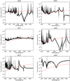 |
Fig. A.1 Photo-ionisation cross-sections for selected Mn I levels with quantum-mechanical data. Top to bottom: a6D3, z6P3*, b4P1, e6S2, x6P3*, and e6D2. Red lines illustrate the hydrogenic cross-sections computed using the effective principal quantum number. |
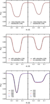 |
Fig. A.2 Comparison of theoretical profiles for Mn I lines at 5394 and 5432 Å in 3D Sun model. Shown are the impact of the resolution of the 3D atmosphere cube (top panel) and the radiative transfer calculations with or without velocity field in opacity (middle panel). The bottom panel demonstrates the line profiles computed for five different solar snapshots selected at regular time intervals. |
Appendix B Additional tables
LS terms of target Mn II ion included in close-coupling expansion.
AUTOSTRUCTURE configuration expansions for Mn II.
Scattering channels correlated to MgH molecular 5Σ+ states, asymptotic energies (J-average experimental values taken from NIST) with respect to the ground state and electronic bound energies with respect to the ionisation limit Mn+(3d54s 5S) + H.
Scattering channels correlated to MgH+ molecular 6Σ+ states, asymptotic energies (J-average experimental values taken from NIST with respect to the ground state and electronic bound energies with respect to the ionisation limit Mn 2+(3d5 6S) + H).
NLTE abundance corrections for MARCS models with Teff = 4500 K and log g = 1.5 dex.
NLTE abundance corrections for MARCS models with Teff = 6000 K and log g = 4.0 dex.
NLTE abundance corrections for MARCS models with Teff = 4500 K and log g = 1.5 dex.
NLTE abundance corrections for MARCS models with Teff = 6000 K and log g = 4.0 dex.
References
- Afşar, M., Sneden, C., Frebel, A., et al. 2016, ApJ, 819, 103 [NASA ADS] [CrossRef] [Google Scholar]
- Amarsi, A. M., & Asplund, M. 2017, MNRAS, 464, 264 [NASA ADS] [CrossRef] [Google Scholar]
- Amarsi, A. M., Lind, K., Asplund, M., Barklem, P. S., & Collet, R. 2016, MNRAS, 463, 1518 [NASA ADS] [CrossRef] [Google Scholar]
- Amarsi, A. M., Barklem, P. S., Asplund, M., Collet, R., & Zatsarinny, O. 2018a, A&A, 616, A89 [NASA ADS] [CrossRef] [EDP Sciences] [Google Scholar]
- Amarsi, A. M., Nordlander, T., Barklem, P. S., et al. 2018b, A&A, 615, A139 [NASA ADS] [CrossRef] [EDP Sciences] [Google Scholar]
- Amarsi, A. M., Barklem, P. S., Asplund, M., Collet, R., & Zatsarinny, O. 2018c, A&A, 616, A89 [NASA ADS] [CrossRef] [EDP Sciences] [Google Scholar]
- Amarsi, A. M., Nissen, P. E., Asplund, M., Lind, K., & Barklem, P. S. 2019, A&A, 622, L4 [Google Scholar]
- Anstee, S. D., & O’Mara, B. J. 1991, MNRAS, 253, 549 [Google Scholar]
- Anstee, S. D., & O’Mara, B. J. 1995, MNRAS, 276, 859 [NASA ADS] [CrossRef] [Google Scholar]
- Asplund, M., Grevesse, N., Sauval, A. J., & Scott, P. 2009, ARA&A, 47, 481 [NASA ADS] [CrossRef] [Google Scholar]
- Badnell, N. R. 1997, J. Phys. B At. Mol. Phys., 30, 1 [NASA ADS] [CrossRef] [Google Scholar]
- Bagnulo, S., Jehin, E., Ledoux, C., et al. 2003, The Messenger, 114, 10 [Google Scholar]
- Barklem, P. S. 2007, A&A, 462, 781 [NASA ADS] [CrossRef] [EDP Sciences] [Google Scholar]
- Barklem, P. S. 2016, A&ARv, 24, 9 [NASA ADS] [CrossRef] [Google Scholar]
- Barklem, P. S. 2017, Astrophysics Source Code Library [record ascl:1701.005] [Google Scholar]
- Barklem, P. S., Piskunov, N., & O’Mara, B. J. 2000, A&AS, 142, 467 [NASA ADS] [CrossRef] [EDP Sciences] [MathSciNet] [PubMed] [Google Scholar]
- Bautista, M. A., & Pradhan, A. K. 1995, J. Phys. B At. Mol. Phys., 28, L173 [CrossRef] [Google Scholar]
- Belyaev, A. K., & Yakovleva, S. A. 2017a, A&A, 608, A33 [NASA ADS] [CrossRef] [EDP Sciences] [Google Scholar]
- Belyaev, A. K., & Yakovleva, S. A. 2017b, A&A, 606, A147 [NASA ADS] [CrossRef] [EDP Sciences] [Google Scholar]
- Belyaevc, A. K., & Voronov, Y. V. 2017c, A&A, 606, A106 [NASA ADS] [CrossRef] [EDP Sciences] [Google Scholar]
- Belyaev, A. K., Yakovleva, S. A., & Barklem, P. S. 2014, A&A, 572, A103 [NASA ADS] [CrossRef] [EDP Sciences] [Google Scholar]
- Belyaev, A. K., Voronov, Y. V., Yakovleva, S. A., et al. 2017, ApJ, 851, 59 [NASA ADS] [CrossRef] [Google Scholar]
- Bergemann, M., & Gehren, T. 2007, A&A, 473, 291 [NASA ADS] [CrossRef] [EDP Sciences] [Google Scholar]
- Bergemann, M., & Gehren, T. 2008, A&A, 492, 823 [NASA ADS] [CrossRef] [EDP Sciences] [Google Scholar]
- Bergemann, M., Lind, K., Collet, R., Magic, Z., & Asplund, M. 2012, MNRAS, 427, 27 [NASA ADS] [CrossRef] [Google Scholar]
- Bergemann, M., Kudritzki, R.-P., Gazak, Z., Davies, B., & Plez, B. 2015, ApJ, 804, 113 [NASA ADS] [CrossRef] [Google Scholar]
- Bergemann, M., Collet, R., Amarsi, A. M., et al. 2017, ApJ, 847, 15 [NASA ADS] [CrossRef] [Google Scholar]
- Berrington, K. A., Burke, P. G., Butler, K., et al. 1987, J. Phys. B At. Mol. Phys., 20, 6379 [NASA ADS] [CrossRef] [Google Scholar]
- Bjørgen, J. P., & Leenaarts, J. 2017, A&A, 599, A118 [NASA ADS] [CrossRef] [EDP Sciences] [Google Scholar]
- Blackwell-Whitehead, R., & Bergemann, M. 2007, A&A, 472, L43 [NASA ADS] [CrossRef] [EDP Sciences] [Google Scholar]
- Bonifacio, P., Spite, M., Cayrel, R., et al. 2009, A&A, 501, 519 [NASA ADS] [CrossRef] [EDP Sciences] [Google Scholar]
- Brueckner, K. A. 1971, ApJ, 169, 621 [NASA ADS] [CrossRef] [Google Scholar]
- Butler, K., & Giddings, J. 1985, Newsletter on Analysis of Astronomical Spectra (London: University of London), 9 [Google Scholar]
- Caffau, E., Ludwig, H.-G., Steffen, M., et al. 2008, A&A, 488, 1031 [CrossRef] [EDP Sciences] [Google Scholar]
- Caffau, E., Maiorca, E., Bonifacio, P., et al. 2009, A&A, 498, 877 [NASA ADS] [CrossRef] [EDP Sciences] [Google Scholar]
- Caffau, E., Ludwig, H.-G., Bonifacio, P., et al. 2010, A&A, 514, A92 [NASA ADS] [CrossRef] [EDP Sciences] [Google Scholar]
- Caffau, E., Ludwig, H.-G., Steffen, M., Freytag, B., & Bonifacio, P. 2011, Sol. Phys., 268, 255 [NASA ADS] [CrossRef] [Google Scholar]
- Carlson, B. 1963, in Statistical Physics, eds. B. Alder, S. Fernbach, & M. Rotenberg (Berlin: Springer), 1 [Google Scholar]
- Carlsson, M. 1992, ASP Conf. Ser., 26, 499 [NASA ADS] [Google Scholar]
- Collet, R., Magic, Z., & Asplund, M. 2011, J. Phys. Conf. Ser., 328, 012003 [NASA ADS] [CrossRef] [Google Scholar]
- Creevey, O. L., Thévenin, F., Boyajian, T. S., et al. 2012, A&A, 545, A17 [NASA ADS] [CrossRef] [EDP Sciences] [Google Scholar]
- Creevey, O., Grundahl, F., Thévenin, F., et al. 2019, A&A, 625, A33 [NASA ADS] [CrossRef] [EDP Sciences] [Google Scholar]
- Danilovic, S., & Vince, I. 2005, Mem. Soc. Astron. It., 76, 949 [NASA ADS] [Google Scholar]
- Danilovic, S., Solanki, S. K., Livingston, W., Krivova, N., & Vince, I. 2016, A&A, 587, A33 [NASA ADS] [CrossRef] [EDP Sciences] [Google Scholar]
- Den Hartog, E. A., Lawler, J. E., Sobeck, J. S., Sneden, C., & Cowan, J. J. 2011, ApJS, 194, 35 [NASA ADS] [CrossRef] [Google Scholar]
- Dravins, D. 1987, A&A, 172, 211 [NASA ADS] [Google Scholar]
- Dravins, D. 1990, A&A, 228, 218 [NASA ADS] [Google Scholar]
- Dravins, D., & Nordlund, A. 1990a, A&A, 228, 184 [NASA ADS] [Google Scholar]
- Dravins, D., & Nordlund, A. 1990b, A&A, 228, 203 [NASA ADS] [Google Scholar]
- Dravins, D., Lindegren, L., & Nordlund, A. 1981, A&A, 96, 345 [NASA ADS] [Google Scholar]
- Drawin, H.-W. 1968, Z. Phys., 211, 404 [NASA ADS] [CrossRef] [EDP Sciences] [Google Scholar]
- Drawin, H. W. 1969, Z. Phys., 225, 470 [NASA ADS] [CrossRef] [Google Scholar]
- Grupp, F. 2004a, A&A, 420, 289 [NASA ADS] [CrossRef] [EDP Sciences] [Google Scholar]
- Grupp, F. 2004b, A&A, 426, 309 [NASA ADS] [CrossRef] [EDP Sciences] [Google Scholar]
- Gudiksen, B. V., Carlsson, M., Hansteen, V. H., et al. 2011, A&A, 531, A154 [NASA ADS] [CrossRef] [EDP Sciences] [Google Scholar]
- Gustafsson, B., Edvardsson, B., Eriksson, K., et al. 2008, A&A, 486, 951 [NASA ADS] [CrossRef] [EDP Sciences] [Google Scholar]
- Holt, R. A., Scholl, T. J., & Rosner, S. D. 1999, MNRAS, 306, 107 [NASA ADS] [CrossRef] [Google Scholar]
- Johnson, J. A. 2002, ApJS, 139, 219 [NASA ADS] [CrossRef] [Google Scholar]
- Karovicova, I., White, T. R., Nordlander, T., et al. 2018, MNRAS, 475, L81 [NASA ADS] [CrossRef] [Google Scholar]
- Kaulakys, B. 1985, J. Phys. B At. Mol. Phys., 18, L167 [NASA ADS] [CrossRef] [Google Scholar]
- Kaulakys, B. 1991, J. Phys. B At. Mol. Phys., 24, L127 [Google Scholar]
- Kunasz, P., & Auer, L. H. 1988, J. Quant. Spectr. Rad. Transf., 39, 67 [Google Scholar]
- Kurucz, R. L., Furenlid, I., Brault, J., & Testerman, L. 1984, Solar Flux Atlas from 296 to 1300 nm (New Mexico: National Solar Observatory) [Google Scholar]
- Leenaarts, J.,& Carlsson, M. 2009, in The Second Hinode Science Meeting: Beyond Discovery-Toward Understanding, eds. B. Lites, M. Cheung, T. Magara, J. Mariska, & K. Reeves, ASP Conf. Ser., 415, 87 [NASA ADS] [Google Scholar]
- Leenaarts, J., Carlsson, M., & Rouppe van der Voort, L. 2012, ApJ, 749, 136 [NASA ADS] [CrossRef] [EDP Sciences] [Google Scholar]
- Lind, K., Bergemann, M., & Asplund, M. 2012, MNRAS, 427, 50 [NASA ADS] [CrossRef] [Google Scholar]
- Lind, K., Amarsi, A. M., Asplund, M., et al. 2017, MNRAS, 468, 4311 [NASA ADS] [CrossRef] [EDP Sciences] [Google Scholar]
- Livingston, W., Wallace, L., White, O. R., & Giampapa, M. S. 2007, ApJ, 657, 1137 [NASA ADS] [CrossRef] [Google Scholar]
- Lodders, K. 2003, ApJ, 591, 1220 [NASA ADS] [CrossRef] [Google Scholar]
- Magic, Z., Collet, R., Asplund, M., et al. 2013, A&A, 557, A26 [NASA ADS] [CrossRef] [EDP Sciences] [Google Scholar]
- Mishenina, T., Gorbaneva, T., Pignatari, M., Thielemann, F.-K., & Korotin, S. A. 2015, MNRAS, 454, 1585 [NASA ADS] [CrossRef] [Google Scholar]
- Nordlander, T., & Lind, K. 2017, A&A, 607, A75 [NASA ADS] [CrossRef] [EDP Sciences] [Google Scholar]
- Nordlund, A., & Dravins, D. 1990, A&A, 228, 155 [Google Scholar]
- Nordlund, Å., & Galsgaard, K. 1995, A 3D MHD code for parallel computers, Tech. rep., Niels Bohr Institute, University of Copenhagen [Google Scholar]
- Nordlund, Å., Stein, R. F., & Asplund, M. 2009, Liv. Rev. Sol. Phys., 6, 2 [Google Scholar]
- O’Mara, B. J. 1976, MNRAS, 177, 551 [NASA ADS] [CrossRef] [Google Scholar]
- Osorio, Y., Barklem, P. S., Lind, K., et al. 2015, A&A, 579, A53 [NASA ADS] [CrossRef] [EDP Sciences] [Google Scholar]
- Plez, B. 2012, Turbospectrum: Code for spectral synthesis, Astrophysics Source Code Library [record ascl:1205.004] [Google Scholar]
- Reetz, J. K. 1999, Sauerstoff in kühlen Sternen und die chemische Entwicklung der Galaxis (Munich, Germany: LMU München) [Google Scholar]
- Reilman, R. F., & Manson, S. T. 1979, ApJS, 40, 815 [NASA ADS] [CrossRef] [Google Scholar]
- Reiners, A., Mrotzek, N., Lemke, U., Hinrichs, J., & Reinsch, K. 2016, A&A, 587, A65 [NASA ADS] [CrossRef] [EDP Sciences] [Google Scholar]
- Rybicki, G. B., & Hummer, D. G. 1991, A&A, 245, 171 [NASA ADS] [Google Scholar]
- Rybicki, G. B., & Hummer, D. G. 1992, A&A, 262, 209 [NASA ADS] [Google Scholar]
- Scott, P., Asplund, M., Grevesse, N., Bergemann, M., & Sauval, A. J. 2015, A&A, 573, A26 [NASA ADS] [CrossRef] [EDP Sciences] [Google Scholar]
- Seitenzahl, I. R., Cescutti, G., Röpke, F. K., Ruiter, A. J., & Pakmor, R. 2013, A&A, 559, L5 [NASA ADS] [CrossRef] [EDP Sciences] [Google Scholar]
- Shetrone, M., Bizyaev, D., Lawler, J. E., et al. 2015, ApJS, 221, 24 [NASA ADS] [CrossRef] [Google Scholar]
- Sneden, C., Cowan, J. J., Kobayashi, C., et al. 2016, ApJ, 817, 53 [NASA ADS] [CrossRef] [Google Scholar]
- Steenbock, W., & Holweger, H. 1984, A&A, 130, 319 [NASA ADS] [Google Scholar]
- Stein, R. F., & Nordlund, A. 1989, ApJ, 342, L95 [NASA ADS] [CrossRef] [PubMed] [Google Scholar]
- Strassmeier, K. G., Ilyin, I., & Steffen, M. 2018, A&A, 612, A44 [NASA ADS] [CrossRef] [EDP Sciences] [Google Scholar]
- Unsöld, A. 1927, Z. Astrophys., 43, 563 [Google Scholar]
- Unsöld, A. 1955, Physik der Sternatmospharen: MIT Besonderer Berucksichtigung der Sonne (Berlin: Springer) [Google Scholar]
- Verner, D. A.,& Yakovlev, D. G. 1995, A&AS, 109, 125 [NASA ADS] [Google Scholar]
- Vitas, N., Viticchiè, B., Rutten, R. J., & Vögler, A. 2009, A&A, 499, 301 [NASA ADS] [CrossRef] [EDP Sciences] [Google Scholar]
- Wise, A. W., Dodson-Robinson, S. E., Bevenour, K., & Provini, A. 2018, AJ, 156, 180 [NASA ADS] [CrossRef] [Google Scholar]
- Yakovleva, S. A., Barklem, P. S., & Belyaev, A. K. 2017, MNRAS, 473, 3810 [Google Scholar]
All Tables
Scattering channels correlated to MgH molecular 5Σ+ states, asymptotic energies (J-average experimental values taken from NIST) with respect to the ground state and electronic bound energies with respect to the ionisation limit Mn+(3d54s 5S) + H.
Scattering channels correlated to MgH+ molecular 6Σ+ states, asymptotic energies (J-average experimental values taken from NIST with respect to the ground state and electronic bound energies with respect to the ionisation limit Mn 2+(3d5 6S) + H).
NLTE abundance corrections for MARCS models with Teff = 4500 K and log g = 1.5 dex.
NLTE abundance corrections for MARCS models with Teff = 6000 K and log g = 4.0 dex.
NLTE abundance corrections for MARCS models with Teff = 4500 K and log g = 1.5 dex.
NLTE abundance corrections for MARCS models with Teff = 6000 K and log g = 4.0 dex.
All Figures
 |
Fig. 1 Grotrian diagram of Mn I atomic system. The energy levels of Mn I are shown with black dashes. The levels are connected by radiative transitions (solid black lines). |
| In the text | |
 |
Fig. 2 Photo-ionisation cross-section of 3d54s2 a 6S ground term of Mn I. The present R-matrix cross-section is depicted by the solid line. The central-field cross-sections of Verner & Yakovlev (1995) and Reilman & Manson (1979) are indicated by the dashed line and square dots, respectively. Above the figure we show the energies of all 3d54s, 3d6, and 3d4 4s2 thresholds. |
| In the text | |
 |
Fig. 3 Neutralisation rate coefficients for Mn+(3d54s 5S) + H− collisions asa function of electronic energy in different excited states of Mn I. The dashed line represents the reduced rate coefficient given by the simplified model. |
| In the text | |
 |
Fig. 4 Neutralisation rate coefficients for Mn2+(3d5 6S) + H− collisions as a function of electronic energy in different excited states of Mn II. The dashed line represents the reduced rate coefficient given by the simplified model. |
| In the text | |
 |
Fig. 5 Excitation (top panel) and ion-pair formation (bottom panel, CT stands for “charge transfer”) rate coefficients for Mn I and Mn II as used in this work and compared to Drawin’s formulae (Drawin 1968, 1969; Steenbock & Holweger 1984). |
| In the text | |
 |
Fig. 6 3D, 1D, and ⟨3D⟩ temperature structures as a function of Rosseland optical depth for benchmark stars. The blue-shaded regions indicate the kinetic temperature distributions in the representative snapshot from the 3D convection simulations. The stellar parameters are given in the inset. We note that ⟨3D ⟩ models are provided only to illustrate the difference between the average structure of the 1D and 3D models, however, the ⟨3D ⟩ are not used in our abundance analysis. |
| In the text | |
 |
Fig. 7 Mn departure coefficients for solar MARCS model atmosphere as a function of optical depth at 5000 Å, computed using DETAIL (top panel) and MULTI (bottom panel) codes. The surface parameters of the Sun, (Teff, log g, and [Fe ∕H]) are given in the figure details. |
| In the text | |
 |
Fig. 8 Mn departure coefficients for model atmosphere of a metal-poor red giant. These were computed using the old Mn atom from Bergemann & Gehren (2007) (top) and the new atom from this paper (middle panel: DETAIL, bottom panel: MULTI). The stellar parameters (Teff, log g, and [Fe ∕H]) are given in the figure titles. |
| In the text | |
 |
Fig. 9 NLTE abundance corrections for Mn I (4030, 4033, 4034, 4783, 4823, 6013, 6016, and 6021 Å) and Mn II (3488 Å) lines. These are computed for a small grid of MARCS model atmospheres representative of dwarfs: Teff = 6000, log g = 4.0 (top panels),and red giants: Teff = 4500, log g = 1.5 (bottom panels) for a range of metallicities from 0 to − 3 dex. Different curves represent the corrections derived using the model atoms with reduced complexity: (a) CH excluded, ignoring the excitation processes by collisions with H atoms; (b) CH0 excluded, ignoring the charge transfer reactions; and (c) CH∕CH0 included with excitation and CT rates from the quantum-mechanical calculations. None of the three models (a–c) include the Kaulakys recipe. |
| In the text | |
 |
Fig. 10 NLTE abundance corrections for Mn I and Mn II lines. These are computed for a small grid of MARCS model atmospheres representative of dwarfs: Teff = 6000, log g = 4.0 (top panels),and red giants: Teff = 4500, log g = 1.5 (bottom panels) for a range of metallicities from 0 to − 3 dex. Different curves represent the corrections derived using two model atoms, one with and the other without collisions derived using the Kaulakys recipe. |
| In the text | |
 |
Fig. 11 Spatially resolved line profiles (left panels) and their bisectors (right panels) for solar disc centre in model snapshot 020. The solid blue curve indicates the line profile extracted from the granule, whereas the red curves correspond to the inter-granular lane. The corresponding surface areas are marked with yellow and blue boxes in Fig. 12. |
| In the text | |
 |
Fig. 12 Monochromatic image of solar granulation at wavelength of 5394 Å at solar disc centre. |
| In the text | |
 |
Fig. 13 Comparison of theoretical profiles for Mn I lines at 4502 and 5394 Å for solar snapshot 020. Top left panel: 1.5D NLTE versus full 3D NLTE. Top right panel: line profiles computed with the 3D data cubes scaled down to the resolution of (x,y,z) = 30, 30, 230 (solid line) and 5, 5, 102 (dashed line). Bottom left panel: full 3D NLTE for the five solar snapshots. Bottom right panel: 3D NLTE profiles versus 1D LTE profiles. |
| In the text | |
 |
Fig. 14 Comparison of 3D NLTE line profiles for selected Mn I lines with observed solar flux spectrum. All model profiles were generated using the same Mn abundance of 5.47 dex. |
| In the text | |
 |
Fig. 15 Mn abundances determined from individual Mn I lines in solar flux spectrum using different models: 1D LTE, 1D NLTE, and 3D NLTE. The solid line denotes the Mn abundances measured in CI chondrites, 5.50 ± 0.03 dex (Lodders 2003). |
| In the text | |
 |
Fig. 16 Line profiles of selected Mn I lines in dwarf and RGB models with metallicities [Fe ∕H ] = −1 (top panels) and [Fe∕H] = − 2 (bottom panels). Thick solid curves correspond to the averaged profiles from five snapshots taken at equidistant time steps. Thin lines are the profiles from individual snapshots. 1D LTE profiles are computed assuming ξt = 1 km s−1. The 1D LTEprofiles would be stronger, if larger ξt values were assumed. Note that different spectral lines of Mn I and Mn II are shown in the panels. |
| In the text | |
 |
Fig. 17 3D NLTE abundance corrections for selected models. |
| In the text | |
 |
Fig. 18 Same as Fig. 16, but thick dotted-dashed brown curves now denote the profiles from 3D LTE calculations for the same five snapshots. |
| In the text | |
 |
Fig. 19 Mn abundances in three metal-poor stars. Left panels: the abundances determined using MAFAGS-OS and 3D models. Right panels: the abundances determined using the MARCS and 3D models. |
| In the text | |
 |
Fig. A.1 Photo-ionisation cross-sections for selected Mn I levels with quantum-mechanical data. Top to bottom: a6D3, z6P3*, b4P1, e6S2, x6P3*, and e6D2. Red lines illustrate the hydrogenic cross-sections computed using the effective principal quantum number. |
| In the text | |
 |
Fig. A.2 Comparison of theoretical profiles for Mn I lines at 5394 and 5432 Å in 3D Sun model. Shown are the impact of the resolution of the 3D atmosphere cube (top panel) and the radiative transfer calculations with or without velocity field in opacity (middle panel). The bottom panel demonstrates the line profiles computed for five different solar snapshots selected at regular time intervals. |
| In the text | |
Current usage metrics show cumulative count of Article Views (full-text article views including HTML views, PDF and ePub downloads, according to the available data) and Abstracts Views on Vision4Press platform.
Data correspond to usage on the plateform after 2015. The current usage metrics is available 48-96 hours after online publication and is updated daily on week days.
Initial download of the metrics may take a while.


